A study of the role of wetlands in defining spatial patterns of near-surface (top 1 m) soil carbon in the Northern Latitudes

(1)

BGD

11, 17967–18002, 2014

The role of wetlands on patterns of soil carbon in Northern

Latitudes

E. M. Blyth et al.

Title Page

Abstract Introduction

Conclusions References

Tables Figures

◭ ◮

Back Close

Full Screen / Esc

Printer-friendly Version

Interactive Discussion

Discussion

P

a

per

|

Discussion

P

a

per

|

Discussion

P

a

per

|

Discussion

P

a

per

|

Biogeosciences Discuss., 11, 17967–18002, 2014 www.biogeosciences-discuss.net/11/17967/2014/ doi:10.5194/bgd-11-17967-2014

This discussion paper is/has been under review for the journal Biogeosciences (BG). Please refer to the corresponding final paper in BG if available.

A study of the role of wetlands in defining

spatial patterns of near-surface (top 1 m)

soil carbon in the Northern Latitudes

E. M. Blyth1, R. Oliver1, and N. Gedney2

1

CEH, Wallingford, Oxfordshire, OX10 8BB, UK 2

Met Office, JCHMR, Wallingford, Oxfordshire, OX10 8BB, UK

Received: 24 September 2014 – Accepted: 11 November 2014 – Published: 19 December 2014

Correspondence to: E. M. Blyth (emb@ceh.ac.uk)

Published by Copernicus Publications on behalf of the European Geosciences Union.

(2)

BGD

11, 17967–18002, 2014

Latitudes

E. M. Blyth et al.

Title Page

Tables Figures

◭ ◮

Back Close

Full Screen / Esc

Discussion

P

a

per

|

Discussion

P

a

per

|

Discussion

P

a

per

|

Discussion

P

a

per

|

Abstract

A study of two observation-based maps (the Harmonised World Soil Database, HWSD and the Northern Circumpolar Soil Carbon Database, NCSCD) of the surface (1 m) soil carbon in the Northern Latitudes (containing the Arctic and Boreal regions) reveal that, although the amounts of carbon estimated to be present in this region are very 5

uncertain, the patterns are robust: both maps have soil carbon maxima that coincide with the major wetlands in the region, as described in the Global Lakes and Wetlands Database, GLWD. In fact, the relationship between near-surface soil carbon and the presence of wetlands is stronger than the relationship with soil temperature and vegetation productivity.

10

These relationships are explored using the land surface model of the UK Hadley Centre GCM: JULES (Joint UK Land Environment Simulator). The model is run to represent conditions at the end of the 20th century. Observed vegetation and phenology are used to define the vegetation, the physical properties of organic soils are represented, the fine-scale topography of the region is included in the parameterisation 15

of the hydrology and as a result the GPP and location of the wetlands of the region are reasonably well simulated using JULES.

Despite this, the soil carbon simulated by the model does not reveal the same patterns or the correlation with the wetland regions that are present in the data. This suggests that the model does not represent sufficiently strongly the suppression of 20

heterotrophic respiration in saturated conditions.

A simple adjustment to the JULES model was made whereby the heterotrophic respiration was reduced by the fraction of the grid that is modelled to be saturated. In effect, for the saturated areas the respiration was zero. This adjustment represents a simple experiment to establish the role of wetlands in defining the spatial patterns of 25

near-surface soil carbon.

The results were an improved predicted spatial pattern of soil carbon, with an increase in the correlation between soil carbon and wetlands although not as strong as

(3)

BGD

11, 17967–18002, 2014

Latitudes

E. M. Blyth et al.

Title Page

Tables Figures

◭ ◮

Back Close

Full Screen / Esc

Discussion

P

a

per

|

Discussion

P

a

per

|

Discussion

P

a

per

|

Discussion

P

a

per

|

suggested by the analysis of the data. This may be because the size of the wetlands was underestimated by the model.

The study suggests that land surface models in general, and JULES in particular, need to establish a stronger moderation of soil respiration in saturated conditions in order that future climate controls on wetlands in the Northern Latitudes will result in the 5

correct changes in soil carbon and carbon emissions.

1 Introduction

1.1 Soil carbon in the Northern Latitudes

Soil organic carbon is the biggest store of terrestrial carbon, but it is a dynamic store. Changes to climate may well affect the ability of the land to store this carbon, either 10

positively or negatively. It is therefore important to understand the way that soil carbon responds to climate.

Models of the land and climate are often used to understand this response. For instance, Todd-Brown et al. (2013) studied a range of coupled Earth System Models which were run for the current climate and then compared the resulting soil carbon 15

maps. There was considerable variation. It is not yet clear whether the range in the modelled estimates of soil carbon were due to the modelled climate (i.e. running too warm/cold or too dry/wet), or to variations in the parameterisation of the terrestrial processes.

In their study, Nishina et al. (2014) analysed a suite of models and their response 20

to a future climate. The results were again very varied. Even for the current climate and using observed climate data rather than the coupled models, there was a range of 1090 to 2650 Pg C and the future climate rendered the land either a net sink or a net source of carbon.

(4)

BGD

11, 17967–18002, 2014

Latitudes

E. M. Blyth et al.

Title Page

Tables Figures

◭ ◮

Back Close

Full Screen / Esc

Discussion

P

a

per

|

Discussion

P

a

per

|

Discussion

P

a

per

|

Discussion

P

a

per

|

There is a clear need for models to be not only improved but also validated against available datasets. In this Section, we discuss previous attempts to do just that and then introduce an idea of how to take this subject forward.

Estimates of stocks of soil organic carbon (SOC) in the Arctic vary considerably – but probably lie in the range of 1400 to 1850 Pg (Tarnocai et al., 2009). This currently 5

represents the largest terrestrial carbon pool, roughly half the total global terrestrial store of carbon. However this may be set to change as the high latitudes warm at twice the rate of the rest of the planet (ACIA, 2005).

In an early review of the state of the carbon stocks and the likely changes that may occur in a future, warmer climate, McGuire et al. (2009) show how potentially sensitive 10

the carbon cycle in the Arctic region is to climate change. For instance, this warming may alter the balance between deposition through increased vegetation growth and release through an increase in respiration.

Early estimates of the changes to the stocks were hampered by a lack of data. Sitch et al. (2007) assessed the carbon balance of the Arctic tundra using remote 15

sensing and process modelling. They found that currently the Tundra shows small net sink of CO₂, which tallied with the remote sensing products which showed a greening of the region in the last couple of decades (Myneni et al., 1997). More recently, Hayes et al. (2011) addressed the question of whether the sink was weakening. They concluded that the models suggest that in recent decades, the rate of carbon 20

sequestration by the Arctic regions is only a fraction of its historic rate (possibly as much as 73 % reduction, although previous values may be an overestimate). This is due to warmer soils resulting in faster decomposition and increased wild-fires.

Subsequently, a comprehensive review of both models (global and regional) and various observational methods (fluxes and inversions) of estimating the carbon 25

balance of the Arctic tundra was made by MacGuire et al. (2012). The observations are inconclusive about whether the region acts as a sink or a source of carbon (a combination of flux data has a mean of−11 and a range of−300 to+90 g C m−2yr−1, while the inversions have a mean of−10 and a range of−36 to+19 g C m−2yr−1). The

(5)

BGD

11, 17967–18002, 2014

Latitudes

E. M. Blyth et al.

Title Page

Tables Figures

◭ ◮

Back Close

Full Screen / Esc

Discussion

P

a

per

|

Discussion

P

a

per

|

Discussion

P

a

per

|

Discussion

P

a

per

|

models indicate a sink but are not conclusive of whether it is a weak or strong sink (the regional models have a mean of −19 and range of −31 to −4 g C m−2yr−1 while the global models have a mean of−9 and a range of−22 to 0 g C m−2yr−1).

1.2 A new way of assessing the data

All of these studies concentrate their analysis on the total carbon budgets and ignore 5

the spatial patterns. Two maps of current soil carbon of the Northern Latitudes have become available: the Harmonised World Soil Database, HWSD and the Northern Circumpolar Soil Carbon Database, NCSCD. These show quite strong spatial patterns across the region. It is possible that correlations of these patterns with factors that might affect soil carbon such as soil temperature, moisture and vegetation productivity 10

and type, may reveal the drivers of soil-carbon accumulation.

Soil carbon changes very slowly, especially in the cold Northern Latitudes. Some of the soil carbon in this region may have been laid down in conditions that are not reflected in current climate patterns. Before attempting to understand the interaction of soil carbon with climate, we need to study the previous several thousand years climate 15

and land history in relation to the processes that affect the soil carbon store.

1.3 Climate and land-history of the Northern Latitudes

During the ice age, over half of the Northern Latitudes (Canada and Western Siberia) was covered in massive ice-sheets, leaving the land surface with no soil of vegetation, just rock. The current organic soil and vegetation cover of the ice-covered areas can 20

only be as old as the Holocene (6000 years old, the date of the Last Glacial Maximum – LGM). The rest of the area has soils that are much older – up to 500 000 years old (see Jones et al., 2010) or, in the case of the Yedoma on the north coast of Siberia, over a million years old (these soils were blown in to the region). The depth of these pre-Holocene soils can be as great as a kilometre deep, although only the top 25

(6)

BGD

11, 17967–18002, 2014

Latitudes

E. M. Blyth et al.

Title Page

Tables Figures

◭ ◮

Back Close

Full Screen / Esc

Discussion

P

a

per

|

Discussion

P

a

per

|

Discussion

P

a

per

|

Discussion

P

a

per

|

several meters are thermally active as the ice-free regions coincide with the permafrost regions, a relic of the pre-Holocene ice ages.

By studying the age of carbon from 6 rivers, Gustafasson et al. (2011) was able to infer the age of the soil carbon in difference regions of Siberia. They are (travelling eastward), Kalix: 560 years, Ob: 3000 years, Yenisey: 1500 years, Lena: 7500 years, 5

Indigirka: 6000 years and Kolyma: 5600 years. This indicates that, roughly speaking, the soil carbon is older in the East. This spatial map of soil carbon age tallies with the history of the ice-sheets in Western Siberia and permafrost in Eastern Siberia, described above.

However, this climate and land history may not be reflected in the surface soil 10

carbon. According to Jones et al., 2010, the rate of accumulation of soil carbon in the Arctic is of the order of 1 mm per year. This estimate tallies with figures from Prentice et al. (1993) of the changes in terrestrial carbon storage since the last glacial maximum. Peat deposits are on average 2–3 m thick, which implies a history of the order a few thousand years. So the observed top 1 m soil carbon store has all been laid down since 15

the ice-age, probably over the last 1000 years. Thus the top 1 m of soil of most of the area represents more recent climate history, not the ancient history. Indeed, despite the contrast in paleo climate conditions across the Arctic, the soil carbon maps of the top 1 m of soil show no evidence of the east–west gradient of the existence of the ice-caps or of the permafrost (Fig. 1a and b). The exception to this is the high-soil carbon of the 20

Yedoma soils in the north east of Siberia. These soils were not generated from local processes, but instead have been blown in. The cold temperatures have preserved them from a much earlier era (1 million years).

The climate history of the past 100 years is more uniform across the region: the average surface temperature in the Northern Latitudes increased by approximately 25

0.1◦C decade−1 (see IPCC, 2013). This information can be used to assess how the carbon stocks have varied over the last century, but only with a model that can successfully establish the processes that have lead to the current patterns of soil carbon.

(7)

BGD

11, 17967–18002, 2014

Latitudes

E. M. Blyth et al.

Title Page

Tables Figures

◭ ◮

Back Close

Full Screen / Esc

Discussion

P

a

per

|

Discussion

P

a

per

|

Discussion

P

a

per

|

Discussion

P

a

per

|

2 Analysing spatial patterns of observations to infer correlations

To facilitate a visual qualitative analysis, we have collated and plotted together a series of maps of variables (temperature, precipitation, plant productivity and vegetation-type) that could a_ffect soil carbon, alongside the two maps of soil carbon available for this region: Harmonized World Soil Database (HWSD) and the Northern Circumpolar Soil 5

Carbon Database (NCSCD) (Tarnocai et al., 2009). Figure 1 shows all of these together and the following sub-sections aim to analyse the spatial correlation of these maps in a qualitative and quantitative way.

2.1 Two soil maps

The two maps of soil carbon down to 1 m show different total amounts of carbon that are 10

assumed to be in the top 1 m of soil. According to Todd-Brown et al. (2013), NCSCD estimates of sol carbon in the top 1 m are between 380 and 620 Pg and HWSD is 290 Pg. This difference in totals is reflected in the maps (Fig. 1a and b): the NCSCD map has a scale that goes up to 80 kg C m−2 while the HWSD maps only goes up to 30 kg C m−2. This difference makes merging of these products a dangerous exercise as 15

the NCSCD only covers northern, colder latitudes and incorrect relationships between soil carbon and temperature can be inferred from the apparent north–south gradient of soil carbon, which is in fact manufactured by the merging of these two products.

Despite the difference in amount, there is a similarity in the spatial pattern of the soil carbon. There are 3 or 4 maxima that occur across these regions in both maps and 20

they seem to coincide with each other. The major exception to this is the high levels of soil carbon in the NCSCD map in East Siberia. This is probably the Yedoma soils referred to in Sect. 1, which were laid down millions of years ago.

(8)

BGD

11, 17967–18002, 2014

Latitudes

E. M. Blyth et al.

Title Page

Tables Figures

◭ ◮

Back Close

Full Screen / Esc

Discussion

P

a

per

|

Discussion

P

a

per

|

Discussion

P

a

per

|

Discussion

P

a

per

|

2.2 Spatial patters of the drivers of soil carbon

The meteorology and plant processes and dominant vegetation type of the area have some clear gradients that can be summarised as follows:

– The temperature (Fig. 1d, from the WFD, Weedon et al., 2011) has a north south gradient being cooler in the north than the south. In addition, there is an east–west 5

gradient in Eurasia where the east is cooler than the West.

– The precipitation (Fig. 1e, from the WFD, Weedon et al., 2011) has an east west gradient in Eurasia, with the east being drier than the west. The Americas have a east to north-west gradient with the north-west being drier than the south-east. There is also a maximum on the west coast of Canada in British Columbia. 10

– The vegetation productivity (Gross Primary Productivity, GPP: Fig. 1f from Jung et al., 2011) follows the rain but with a reduction in the very cold regions of the north. This results in a maximum in the mid latitudes (45 to 60) in Europe and spreading across the forests of Siberia. In the American continent, there is a maximum in south eastern Canada and on the west coast in British Columbia. 15

– The vegetation cover (Fig. 1g) has a band of needle leaf trees at a latitude between 60 and 65◦N, with grasses (representing grass and crops) south of that band and dominant bare soil with some shrubs above that band.

None of these patterns bear any resemblance to the patterns of soil carbon described in Sect. 2.1 with the 3 or 4 patches of soil carbon maxima. Not only is it unlikely that any 20

single driving variable is responsible for soil carbon, it is also unlikely that combinations of these driving variables could be found that would pick out the soil carbon maxima shown in Fig. 1a and b.

(9)

BGD

11, 17967–18002, 2014

Latitudes

E. M. Blyth et al.

Title Page

Tables Figures

◭ ◮

Back Close

Full Screen / Esc

Discussion

P

a

per

|

Discussion

P

a

per

|

Discussion

P

a

per

|

Discussion

P

a

per

|

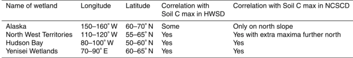
2.3 Spatial patterns of wetlands

Figure 1c shows the maps of wetlands given by Lehner and Döll (2004): the Global Lakes and Wetlands Database (GLWD). It is clear from this map that there are 4 large wetland areas in this study area. Table 1 gives their location and the name used in this paper: Alaska, North West Territories, Hudson Bay and Yenisei Wetlands.

5

From a visual inspection, it can be seen that the areas of the major wetlands in the Northern Latitudes do correlate to the areas of the soil carbon maxima. The table highlights where these correlations are strongest.

To some extent this correlation may not be a coincidence as the soil carbon maps will use information about the landscape to extend the point measurements of soil carbon 10

up to the global scale. So that the presence of wetlands may inform the soil carbon maps itself. However, even if this is the case, the soil carbon map makers, whether objectively or subjectively, consider wetlands to be a prime factor in determining the soil carbon and this correlation is therefore something that the models ought to be able to replicate.

15

2.4 Analysis of spatial patterns

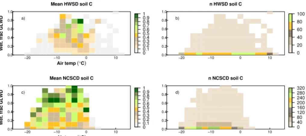
To better quantify the correlation between soil carbon and possible drivers, in Fig. 2 we have plotted the soil carbon against air temperature (which represents the closest thing we have to the observed soil temperature over the top 1 m) and wetland extent shown in Fig. 1c. We have also plotted the number of cells that make up this plot, to highlight 20

that the results are based on a very small sample of data and so to urge caution. This plot emphasises what we have already seen in the maps, that there is a strong correlation between soil carbon and wetlands that is not seen for instance in the temperature. This result informs the model experiment described in Sect. 3 and the analysis of results in Sect. 4.

25

A visual inspection (more analysis is given in Sect. 4) of these plots highlight the functional relationship between soil carbon and temperature and wetlands. Because

(10)

BGD

11, 17967–18002, 2014

Latitudes

E. M. Blyth et al.

Title Page

Tables Figures

◭ ◮

Back Close

Full Screen / Esc

Discussion

P

a

per

|

Discussion

P

a

per

|

Discussion

P

a

per

|

Discussion

P

a

per

|

they do not depend on the spatial location, they can be used to analyse model outputs where the location of the wetlands may be in errors for reasons that do not concern this study or affect the conclusions. The relationship portrayed by these plots can therefore be compared directly to the observations.

3 Method and modelling

5

3.1 Overall methodology

The aim of this paper is to establish the relative importance of the temperature and moisture fields on the spatial patterns of carbon accumulated in the soils in the Northern Latitudes. It is not possible to do this by studying correlations, as they cannot diagnose cause and effect. Instead, a model that explicitly represents 10

the evolution of soil carbon as it responds to climate, via an interaction with the hydrology and vegetation processes of the region can be used. A land surface model such as JULES (Joint UK Environment Simulator – see Appendix A) is ideal as it represents the soil carbon gains and losses via changes in litter-fall and heterotrophic respiration respectively explicitly. Heterotrophic respiration is predominantly dependent 15

on temperature and moisture which are modelled explicitly, although there are large uncertainties in the relationships. Other factors such as disturbance (Grosse et al., 2011) and fire are not included in the land–surface model used in this study. However, the pattern matching discussed in Sect. 2 to highlights the importance of wetlands in this region, which is therefore the focus of our study.

20

The overall methodology is to drive the model with observed meteorological forcing for the 20th century (using the WATCH Forcing Data, WFD, see Weedon et al., 2011), reaching an equilibrium soil carbon that is representative of the last thousand years and then to run the model forward for the full 20th century to represent conditions at the end of the 20th century when the observations of soil carbon were taken. The 25

method is described briefly in Sect. 3.3 and more fully in Appendix A. By introducing

(11)

BGD

11, 17967–18002, 2014

Latitudes

E. M. Blyth et al.

Title Page

Tables Figures

◭ ◮

Back Close

Full Screen / Esc

Discussion

P

a

per

|

Discussion

P

a

per

|

Discussion

P

a

per

|

Discussion

P

a

per

|

different parameterisations of the dependencies of the soil respiration to moisture and temperature and then comparing the patterns of resulting soil carbon to the data, we aim to distinguish the key factors in determining the accumulation of soil carbon in this region.

Study of the correlations of the observed soil carbon maps with the soil temperature 5

and moisture conditions (see Sect. 2) suggests that one of the key processes controlling near-surface soil carbon is the presence of wetlands, wherein the saturated soils suppress decomposition. In the following descriptions, there will be a focus on that aspect of the model. An ideal mechanistic wetland model is not yet available within JULES, but in this study, we are able to carry out model simulations with 10

a parameterised wetland model. This enables us to test the hypothesis that wetlands are important to near-surface soil carbon, and the results can be used to prioritise model development.

3.2 Model setup

Choices have to be made about how to set the model up. In this case we chose to use 15

observed land cover maps and observed variations in leaf area so that the only aspect land surface controlled by the model is the soil temperature and moisture.

We followed the method proposed by Lawrence and Slater (2008) for including organic soil parameters into the Brooks and Corey soil hydraulic equations and applied the LSH (based on Topmodel) rainfall-runoffmodule within JULES. The carbon 20

contents which are used to define areas of organic soil are taken from the observed soil carbon maps (see Fig. 1) and the topographic index calculated using a 1 km topographic database. The model options for soil respiration dependency on soil temperature were set up as described in Jones et al. (2005), which uses the soil temperature at 20 cm depth (second soil layer in the model).

25

The model diagnoses the wetland fraction of each grid cell as a function of the mean soil moisture in the cell and the topographic index. This is used to alter the soil moisture moderator of heterotrophic respiration as described in Sect. 3.4.

(12)

BGD

11, 17967–18002, 2014

Latitudes

E. M. Blyth et al.

Title Page

Tables Figures

◭ ◮

Back Close

Full Screen / Esc

Discussion

P

a

per

|

Discussion

P

a

per

|

Discussion

P

a

per

|

Discussion

P

a

per

|

3.3 Modelling soil C and spin-up

The overall methodology adopted is to find the equilibrium soil carbon based on the climate and atmospheric CO2 concentration of the first two decades of the 1900s.

The equilibrium is where there is a balance between the modelled litter-fall from the vegetation fields (specified from satellite data), and the modelled soil respiration. This 5

“equilibrium” state is then used as the starting point for a 100 year simulation with the observation-based global climate including changes in the atmospheric CO₂. This is called the “transient” run. The patterns of soil carbon at the end of the 1900s are then analysed.

Simulation of soil C storage by JULES is described in detail by Clark et al. (2011). 10

Briefly, in JULES, soil C stocks are modelled as a balance between C inputs from vegetation litterfall and C losses from soil respiration which returns CO2 to the

atmosphere. JULES simulates soil C decomposition using first-order kinetics that determines the turnover rates of four (labelled “i” in the following equation) soil C pools. These four pools comprise decomposable (DPM) and resistant plant material 15

(RPM), microbial biomass (BIO), and humus (HUM). Decomposition is determined by a specific respiration rate for each pool, by the carbon content of each pool,Ci, and by

temperature,Ft and moisture availability Fs and the vegetation fraction Fv (see Eqs. 1

to 5).

R_i =κ_iC_iFtFsFv (1)

20

whereκis 10 for DPM, 0.3 for RPM, 0.7 for BIO and 0.02 for HUM.

The soil C pools have very slow response times, especially in the high Northern latitudes where short seasons and low temperatures slow the system down. This means achieving an equilibrium state in these regions can take thousands of years, which is both time and computationally expensive. Therefore, we use an “accelerated 25

decomposition” procedure to find our C equilibrium state that is described in Koven et al. (2011) and Thornton and Rosenbloom (2005). The principle is based on the fact

(13)

BGD

11, 17967–18002, 2014

Latitudes

E. M. Blyth et al.

Title Page

Tables Figures

◭ ◮

Back Close

Full Screen / Esc

Discussion

P

a

per

|

Discussion

P

a

per

|

Discussion

P

a

per

|

Discussion

P

a

per

|

that the respiration (output) is linearly proportional to the value ofκand the total amount of C in the store and the litterfall (input) is independent of C andκ. This means that if the value ofκis reduced by a factor, then the value of C will be increased by the same factor, leaving the value ofR unchanged. The time the store takes to reach equilibrium is defined byκ, which is the turnover rate of the store. These vary by a huge amount 5

(see above) with the slowest (HUM) at 3 orders of magnitude slower than the fastest (DPM). In JULES, we therefore set all the turnover rates to equal the fastest rate (10 per annum), and then, at the end of the equilibrium run, scale the carbon stores with the ratio of the values of κ. (Tests were performed with a full spin-up leaving the κ values un changed, and the results were the same). The methodology is summarised 10

in Appendix A.

3.4 Model equations

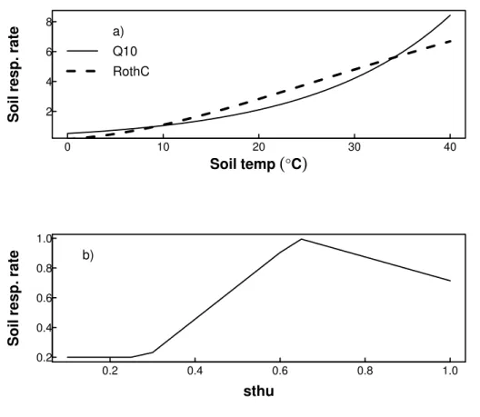
There are two possible options in the model for the temperature moderator. One is termed theQ₁₀function and is given by

Ft=Q

(Ts−282.4)/10

10 (2)

15

The other is termed the RothC function and is given by

Ft=

47.9

1+e106/(T_s−254.85) (3)

These temperature functions are graphically illustrated in Fig. 3. The soil moisture moderator is a piece-wise linear function given by

Fs=

   

  

1−0.8(s−s₀) fors > s₀

0.2+0.8s−smin

s0−smin

fors_min< s≤s₀

0.2 fors≤s_min

(4) 20

(14)

BGD

11, 17967–18002, 2014

Latitudes

E. M. Blyth et al.

Title Page

Tables Figures

◭ ◮

Back Close

Full Screen / Esc

Discussion

P

a

per

|

Discussion

P

a

per

|

Discussion

P

a

per

|

Discussion

P

a

per

|

wheres is the unfrozen soil moisture, so the optimum soil moisture:s0=0.5(1+sw)

wheresw is the wilting point andsmin=1.7sw. The upper soil moisture branch of this

function (wheres > s0) aims to represent the suppression of heterotrophic respiration

as the soil moisture approaches saturation. This function is graphically illustrated in Fig. 3.

5

The impact that vegetation cover has is given by

Fv=0.6+0.4(1−v) (5)

wherev is the vegetation cover. See Clark et al. (2011) for details.

These functions use global constants. Values forQ10, for example, are determined

because they generate the right atmospheric CO2 concentrations. There is some

10

uncertainty of these values, and to some extent they can be tuned to get the required results. The shapes of the curves however cannot be tuned and they, with the spatial patterns of soil temperature and moisture, determine the final spatial patterns of soil carbon. We will explore these in the following section. The two temperature functions are used throughout. The soil moisture function in particular may be very uncertain. 15

Falloon et al. (2011) showed that land surface models use a wide variety of functions for this moderation and we introduce yet another variation here in this study (see Sect. 3.5).

3.5 Modelled wetland fraction and impact on heterotrophic respiration

Wetlands are generally a sub-grid phenomenon since they do not cover the full 50 km 20

square grid box. In the JULES model they are inferred from the mean soil moisture as the ratio of the mean soil moisture in the top 10 cm to the saturated soil moisture. It is possible to either use the unfrozen fraction or the total soil moisture. In these analyses we use the total soil moisture.

To explore the role of wetlands on soil carbon, a simple model experiment was 25

performed. The model was run as described above, but an alteration was made whereby the area of the grid that was deemed to be a wetland (Fwet=s/ssat), wheressat

(15)

BGD

11, 17967–18002, 2014

Latitudes

E. M. Blyth et al.

Title Page

Tables Figures

◭ ◮

Back Close

Full Screen / Esc

Discussion

P

a

per

|

Discussion

P

a

per

|

Discussion

P

a

per

|

Discussion

P

a

per

|

would have zero respiration. The grid box respiration including the effect of wetlands, Rw, was therefore given by:

Rw=R·(1−Fwet) (6)

4 Results

4.1 Comparison of model result with observed wetlands and GPP

5

It is not possible to validate every aspect of the model, as either we do not have the data to do so, or it is not relevant to the question we are studying. For instance, we do not have a readily available map of soil temperature across this region. However, since the model is being driven by observation-based data on temperature at 2 m, it is likely that the soil temperature will not be too different from the 2 m temperature and 10

therefore not that far wrong.

Other aspects of the model however can be compared with observations. An observational based map of wetlands is available (Lehner and Döll, 2004: the Global Lakes and Wetlands Database, GLWD) which can be used to compare with the model. In Sect. 2, the observation-based map of wetlands, frozen and unfrozen, was shown 15

in Fig. 1c. It was clear from that map that there are 4 large wetland areas in this study area. Table 1 gives their location and the name used in this paper: Alaska, North West Territories, Hudson Bay and Yenisei Wetlands.

In Sect. 2, Fig. 1f showed some maps of observed gross primary productivity (GPP) derived from Flux data (Jung et al., 2011) which can be used to assess if the spatial 20

patterns modelled carbon inputs to the soil are about right. They had a maximum in the mid latitudes (45 to 60) in Europe and spreading across the forests of Siberia. In the American continent, there was a maximum in south eastern Canada and a much smaller maximum on the west coast in British Columbia.

The same maps, but this time model derived, are shown in Fig. 4. Note that the 25

(16)

BGD

11, 17967–18002, 2014

Latitudes

E. M. Blyth et al.

Title Page

Tables Figures

◭ ◮

Back Close

Full Screen / Esc

Discussion

P

a

per

|

Discussion

P

a

per

|

Discussion

P

a

per

|

Discussion

P

a

per

|

observation-based Fig. 1c, while the scale for the GPP is the same in both Figs. 4b and 1f.

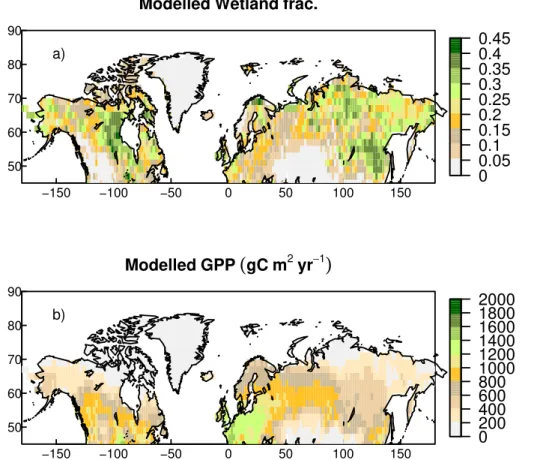
Figure 4a shows that the wetlands in the model are to some extent reproduced in the model: the key wetland areas are captured with the Alaska and Hudson Bay wetlands being modelled reasonably well. The North West Territories wetlands are 5

underestimated and instead the model simulates an extensive wetland area to the east of that region. The Yenisei wetlands are captured, but again extensive extra wetlands areas are simulated to the east of that region.

However, the modelled wetlands only cover about half the grid boxes as a maximum while the observed wetlands often fill the grid. This disparity of the size of the wetland 10

areas (as opposed to their extent, which is over estimated) will a_ffect the resulting modelled results and tend to lead to an underestimate of the soil carbon. It is possible that the wetlands are underestimated due to the lack of lateral flow in the model, so the only water received within a grid cell comes from the precipitation and none from the upstream rivers.

15

It is not the intention in this study to model the exact location of the wetlands. Rather (and later in this section) we wish to model the impact that wetlands have on soil carbon. Therefore this mismatch in location does not affect our analysis and it is beneficial that there are a number of wetland areas at the same latitudes as the observations so that we can compare like with like with the e_ffect of temperature and 20

soil moisture on soil carbon.

Figure 4b shows the modelled GPP from the JULES model. A comparison with observations (Jung et al., 2011 as described above) suggests that the simulated GPP matches reasonably well, with maxima in the temperate Europe (latitudes 45 to 60) and spreading into Siberia. The model also captures the maximum in southern Canada, 25

although it is lower on the coast. The greatest anomaly is that the model simulates large values of GPP on the west coast of Canada in British Columbia compared to the observations. The model also does not capture some of the maximum values observed in west Europe (UK and France). However, the spatial patterns are well

(17)

BGD

11, 17967–18002, 2014

Latitudes

E. M. Blyth et al.

Title Page

Tables Figures

◭ ◮

Back Close

Full Screen / Esc

Discussion

P

a

per

|

Discussion

P

a

per

|

Discussion

P

a

per

|

Discussion

P

a

per

|

captured and from this we can assume that the modelled carbon inputs to the soil are reasonably correct, and that the heterotrophic respiration term will contribute the largest uncertainty to the equilibrium soil carbon.

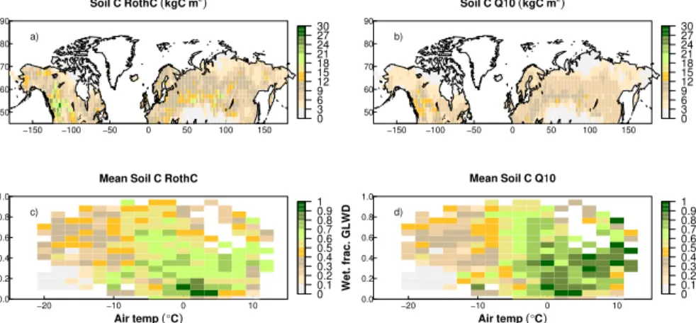
4.2 Analysis of modelled spatial patterns of soil carbon

In the first instance, the standard version of JULES using the soil moisture and 5

temperature functions described in Sect. 3 is used to simulate the soil carbon in this region. The results for the two temperature functions, Q10 and RothC are shown in

Fig. 5.

An initial viewing of the soil carbon suggests that the amounts are too low. The maximum modelled soil carbon using the RothC formula is only 30 kg C m−2 and for 10

theQ10 formula only 20 kg C m

−2

while the observed values reach 40 kg C m−2 in the HSWD dataset and up to 80 kg C m−2for the NCSCD dataset.

As mentioned previously, the total amounts of carbon anyway are uncertain and it is possible to tune the model to fit the values. So to some extent this result has little meaning.

15

The spatial patterns however are more robust in the data and the ability of the model to match that is the basis for this analysis. The modelled soil carbon shows little spatial correlation with the two observed maps. The RothC model result shows a maximum in the western Canada, the British Columbia region which had a high value of GPP, and some maxima in Eastern Europe at the latitude of 60◦. TheQ10has the same locations

20

for their maxima but the values are much lower.

To assess the causes of the patterns, the same plots were made of the soil carbon against the modelled wetland fraction and the air temperature and shown in Fig. 5c and d. This was done so that the results are insensitive to the modelled location of wetlands (see Sect. 5.2) which may be in error. The results of this analysis compared 25

to the same analysis with the observations show a distinct lack of sensitivity to the wetlands which was such a strong part of the observations (see Fig. 2a and c).

(18)

BGD

11, 17967–18002, 2014

Latitudes

E. M. Blyth et al.

Title Page

Tables Figures

◭ ◮

Back Close

Full Screen / Esc

Discussion

P

a

per

|

Discussion

P

a

per

|

Discussion

P

a

per

|

Discussion

P

a

per

|

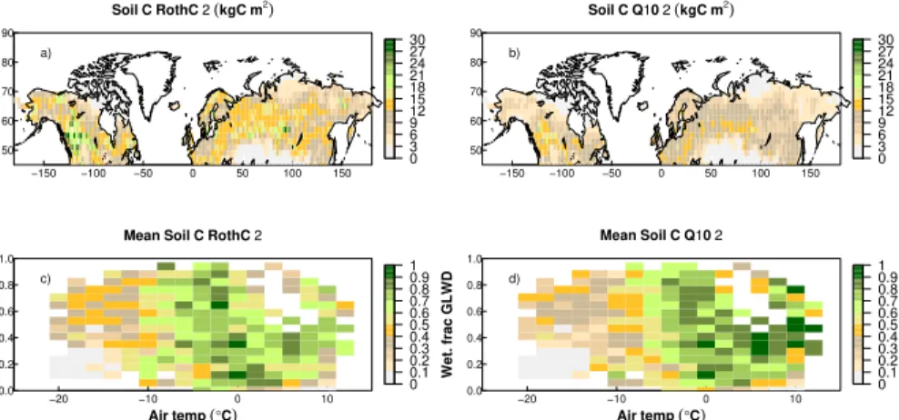
4.3 New wetland-function on heterotrophic respiration

A simple representation of the impact of wetlands on heterotrophic respiration: that is completely suppresses it, was made in the model and the results are shown in Fig. 6.

Figures 6 a and b show the new spatial maps of soil carbon using the two soil temperature functions RothC andQ10 and the new wetland function, Eq. (6) It is clear

5

that the high values of soil carbon in Western Canada are still present in this simulation and altering the response to wetland areas has not affected this region (which is to be expected). However, we can also see an increase in the soil carbon in some of the key wetland areas. For the RothC simulation, Alaska has an increase, parts of the North West Territories, the Hudson Bay close to the coast, and a slight increase in the Yenisei 10

wetland region. For theQ10 simulation, a similar but less pronounced result.

The plots of the soil carbon against the modelled wetland fraction and the air temperature (Fig. 6c and d) give a picture of the advances that have been made. While the high levels of soil carbon at high temperatures are still there (cf Fig. 5c and d), there is now an increase of soil carbon in the areas where wetlands are modelled, which is 15

beginning to approach the patterns displayed by the observations (Fig. 2a and c). To get a clearer idea of the role of wetlands and soil temperature on soil carbon, the results from the wetland/temperature plots were analysed in a linear form (see Fig. 7). The mean values of soil carbon against wetland fraction and against air temperature were analysed. The statistical methods used are described in Appendix B1.

20

The observations (Fig. 7a and b) show, as inferred from the maps, that there is a clear correlation between soil carbon and wetland fraction (to some extent this is not coincidental as the soil carbon maps are inferred from the wetland map) and a non-linear relation with air temperature. The reduction of soil carbon with high temperatures is due to the increase of respiration (see Fig. 3) while the reduction with 25

low temperature is due to the implicit reduction in GPP.

It is interesting to note is how the models compare with this very simple analysis. The temperature functions are similar but have an optimum at about 0◦C for RothC

(19)

BGD

11, 17967–18002, 2014

Latitudes

E. M. Blyth et al.

Title Page

Tables Figures

◭ ◮

Back Close

Full Screen / Esc

Discussion

P

a

per

|

Discussion

P

a

per

|

Discussion

P

a

per

|

Discussion

P

a

per

|

and about 5 to 10◦C forQ10, which is much higher than the observations which both

have an optimum at temperatures below freezing.

The modelled response to normalised wetland fraction is also very different: there is a slight negative correlation between soil carbon and soil moisture in the default version of JULES, and a positive, but small, correlation in the Wetland-respiration-suppression 5

version of JULES. The low value of the slope is to some extent explained by the fact that the wetlands are half the size (cover half the fraction of the grid) compared to the observed wetlands. Since thex axis is the normalised wetland fraction this will result in a lower slope of the curve.

It would be possible to tune the results to fit the observations more nearly, but since 10

there are aspects to the model (such as wetland size) that are not the subject of this study, it was adequate to show that the patterns rather than amount of carbon can be reproduced with a simple treatment of wetland fraction in the model.

5 Discussion of missing processes in land surface models

5.1 Missing processes: hydrology

15

In Todd-Brown et al. (2013) studied the causes of variation in soil carbon simulations from the Earth system models. The total amount of soil carbon simulated was well within the uncertainty of the data (which itself is very large – see above), but the distribution bore no resemblance to either of the global-soil carbon datasets available. In general, the models seem to show a greater soil carbon amount in East Siberia than 20

West Siberia in strong contrast to the observations. The authors suggest that this may be due to the fact that the model soil carbon is too dependent on the temperature of the soil (the cold regions store carbon, the warmer regions have a reduced soil carbon due to higher respiration rates) and that more small-scale impacts of the land surface are necessarily ignored when using models of this scale.

25

(20)

BGD

11, 17967–18002, 2014

Latitudes

E. M. Blyth et al.

Title Page

Tables Figures

◭ ◮

Back Close

Full Screen / Esc

Discussion

P

a

per

|

Discussion

P

a

per

|

Discussion

P

a

per

|

Discussion

P

a

per

|

The processes that have been ignored are mainly related to the local and large scale hydrology. The soil wetness plays a major role in the soil carbon decomposition and therefore on the retained soil carbon. The Northern Latitudes are very wet as can be witnesses in the satellite products of the area (see Prigent et al., 2012) and few models are able to represent this is the subject of much research and it is likely that 5

improvements can be made in the near future. For instance the soil characteristics of these regions are often peaty and this soil type is not often included in land surface models. The inundation of the large rivers that traverse these flat regions is not modelled, but there are new model versions that include this process.

As mentioned previously, there is large uncertainty in the role that soil moisture 10

plays in heterotrophic respiration (see Falloon et al., 2011) and this paper highlights the uncertainty at the very high end of soil moisture where is becomes saturated. Wania et al. (2009) also modify the moisture response specifically for boreal wetlands. Given the sensitivity of simulated soil respiration to these functions, and the inherently di_fferent properties of permanently inundated soils, it is not surprising that using global 15

constants to simulate soil C losses fails to capture the observed spatial heterogeneity.

5.2 Missing processes: microbiology

JULES does not consider the role of microbes in SOC decomposition, as this is implicit in the pool specific decay constants used. Recent work, however, suggests that explicitly representing microbial processes would allow simulation of 20

feedback mechanisms between the environment and microbial communities, improving estimates of SOC change in the future and feedbacks in the carbon–climate system (Allison et al., 2010; Wieder et al., 2013).

Mahecha et al. (2010) find a global convergence ofQ10values for respiration across

terrestrial biomes of ∼1.4. They suggest that factors that co-vary with temperature

25

can confound the estimation of Q10 values, leading to oversensitivity of ecosystem

metabolic processes to temperature. Consequently they argue for the determination and use of intrinsic rather than apparent temperature dependencies of respiration.

(21)

BGD

11, 17967–18002, 2014

Latitudes

E. M. Blyth et al.

Title Page

Tables Figures

◭ ◮

Back Close

Full Screen / Esc

Discussion

P

a

per

|

Discussion

P

a

per

|

Discussion

P

a

per

|

Discussion

P

a

per

|

Currently, in the majority of land-surface models this is not possible, since most do not include sufficient process representation of soil C turnover to allow consideration of confounding factors such as microbial/enzymatic controls of decomposition.

It is possible that improving the microbial modelling in land surface model (and JULES in particular) would improve the spatial patterns of soil carbon. The Fig. 7 5

showed that the modelled response to soil temperature was not the same as the observed, as very briefly discussed in Sect. 4.3.

6 Conclusions

This study showed that there is a correlation between the spatial maps of observed soil carbon and the observed wetlands. The correlation with temperature was weak. 10

The weak correlation with temperature may be due to fact that the positive effect of an increase in vegetation productivity in the warmer southern parts of this region on soil carbon inputs are cancelled by the increased soil respiration in these warmer regions.

The stronger correlation with wetland fraction implies a significant role of wetlands in 15

the long term accumulation of soil carbon in the Northern Latitudes. This may be due to the suppression of soil respiration due to the saturated conditions, which over even a small area has a large impact on the total soil carbon of the region.

To explore the way the wetlands affect soil carbon, a land surface model was used to reproduce the equilibrium soil carbon in the Northern Latitudes. This model is able 20

to predict with some accuracy the location of the wetlands and the spatial patterns of vegetation productivity. However, in its default setting, it is unable to predict the co-location of the high soil carbon with the wetland fraction.

The model was only able to reproduce a similar correlation between soil carbon and wetland fraction if an additional soil-respiration suppression factor was added to the 25

existing code.

(22)

BGD

11, 17967–18002, 2014

Latitudes

E. M. Blyth et al.

Title Page

Tables Figures

◭ ◮

Back Close

Full Screen / Esc

Discussion

P

a

per

|

Discussion

P

a

per

|

Discussion

P

a

per

|

Discussion

P

a

per

|

The overall soil carbon in the model was underestimated, but the study did not attempt to calibrate the model any further. Instead, this study concludes by highlighting the impact of the wetlands on the spatial correlation of wetlands and soil carbon.

This study highlights the role of hydrology and its interaction with biogeochemistry on the carbon budget of this region. The importance of wetlands on soil carbon is of great 5

significance to many scientific questions. For instance, as the Northern Latitudes warm over the coming decades, the presence of wetlands is likely to change. The increased warming may dry out the area, while the melting of the permafrost may cause more wetlands to be created. The impact that this has on the total carbon budget needs to be understood.

10

The results can only be appropriate only to the Northern Latitudes where the soil carbon processes are dominated by the cold temperatures that suppress the soil respiration. Tropical regions may have a completely different correlation with temperature, vegetation and soil moisture.

Appendix A:

15

Spin up:

We used the Used WATCH-ER40 met. forcing 2◦×2◦1901 to 1910 period of forcing

used for spin-up.

To get the vegetation carbon up to equilibrium we:

– spin the equilibrium-vegetation for 1901 to 1910×10 cycles,

20

– spin the dynamic-vegetation for 1901 to 1910×10 cycles.

To get the soil carbon up to equilibrium we then:

– changed decomposition rates to fastest pool,

– spin Accelerated Decomposition 1901 to 1910×10 cycles,

(23)

BGD

11, 17967–18002, 2014

Latitudes

E. M. Blyth et al.

Title Page

Tables Figures

◭ ◮

Back Close

Full Screen / Esc

Discussion

P

a

per

|

Discussion

P

a

per

|

Discussion

P

a

per

|

Discussion

P

a

per

|

– Multiply soil C pools by scale factors to get back to the fully spun-up soil C pool sizes.

Spin-up uses a fixed 1901 CO2concentration.

The transient run is from 1910 to 2001 and uses a changing CO₂ – monthly atmospheric CO2concentration. 1958 onwards from Mauna Loa (www.esrl.noaa.gov/

5

gmd/ccgg/trends/). These data are monthly. 1901 to 1958 from SRES A2 scenario. Analysis period for model output was 1991 to 2001.

Appendix B:

B1 Statistical analysis

For plotting and analysis, observed and modelled wetland fraction and air temperature 10

were binned, and the mean soil C calculated for each bin. Observed and modelled soil C and wetland fraction were normalised for easier comparison between the two, given the large differences in modelled and observed values. Observed and modelled data were analysed using linear regression or ANCOVA as appropriate, using the statistical software R (R Development Core Team, 2011). Levels of significance for explanatory 15

variables were taken asP <0.05.

B2 Results (see stats_plots.pdf)

1. Observed Soil C (NCSCD = red triangles; HWSD=black circles) “v” Observed Wetland fraction (GLWD) (top left plot).

A significant positive correlation between soil C and wetland fraction was found 20

in both observed datasets (NCSCD soil C=0.40+0.41·wetl.frac, r2=0.72, F-test: F_1,7=18.21,P =0.003; HWSD soil C=0.11+0.28·wetl.frac,r2=0.6, F_1,7=

10.50,P =0.014).

(24)

BGD

11, 17967–18002, 2014

Latitudes

E. M. Blyth et al.

Title Page

Tables Figures

◭ ◮

Back Close

Full Screen / Esc

Discussion

P

a

per

|

Discussion

P

a

per

|

Discussion

P

a

per

|

Discussion

P

a

per

|

2. Observed Soil C (NCSCD=red triangles; HWSD=black circles) “v” Observed Air Temperature (top right plot).

The relationship between soil C and air temperature showed significant non-linearity, and was best described by a quadratic model for both datasets (NCSCD F1,10=21.24, P =0.001; HWSD F1,14 =18.45, P =0.0007). Both

5

datasets generally showed higher soil C at lower temperatures (<0◦C), with soil C declining at higher temperatures (>0◦C) and extreme low temperatures (<−15◦C).

3. Modelled Soil C “v” Modelled Wetland fraction (bottom left plot)

ANCOVA analysis (analysis of covariance) showed that modelled soil C from all 10

model runs (RothC and Q10 temperature response functions, with and without

the wetland respiration rate modifier) were significantly correlated with wetland fraction, but the direction of the relationship changed if the model run was made with or without the wetland respiration rate modifier (RothC F_1,17₌7.48, P =0.015; Q10 F1,17=5.91, P =0.027). Using the RothC or Q10 temperature

15

response function and no rate modifier, modelled soil C decreased with increasing wetland fraction, whereas switching on the respiration rate modifier in the model generated increased soil C with increasing wetland fraction.

4. Modelled Soil C “v” Air temperature (bottom right plot)

All models display significant non-linearity in the response of modelled soil C to 20

air temperature:

RothC (black) – (F1,14=60.08,P =1.97×10

−6

)

RothC 2 (red) – (F1,14=40.11,P =1.85×10

−5

) Q10 (green) – (F1,14=16.53,P =0.001)

Q₁₀ 2 (blue) – (F_1,14=12.89,P =0.003) 25

(25)

BGD

11, 17967–18002, 2014

Latitudes

E. M. Blyth et al.

Title Page

Tables Figures

◭ ◮

Back Close

Full Screen / Esc

Discussion

P

a

per

|

Discussion

P

a

per

|

Discussion

P

a

per

|

Discussion

P

a

per

|

Acknowledgements. This work was funded by the NERC grant: the response of the Arctic

regions to changing climate. Grant number NE/H000224/1

We gratefully acknowledge the help of colleagues in re-gridding various datasets for this analysis: Garry Hayman and Charles George. Discussions with colleagues have also been really useful: Richard Harding, Eleanor Burke and Sarah Chadburn.

5

References

ACIA: Impacts of a Warming Arctic: Arctic Climate Impact Assessment, ACIA Overview report, Cambridge University Press, Cambridge, 140 pp., 2004.

Allison, S. D., Wallenstein, M. D., and Bradford, M. A.: Soil-carbon response to warming depends on microbial physiology, Nat. Geosci., 3, 336–340, doi:10.1038/ngeo846, 2010.

10

Clark, D. B., Mercado, L. M., Sitch, S., Jones, C. D., Gedney, N., Best, M. J., Pryor, M., Rooney, G. G., Essery, R. L. H., Blyth, E., Boucher, O., Harding, R. J., Huntingford, C., and Cox, P. M.: The Joint UK Land Environment Simulator (JULES), model description – Part 2: Carbon fluxes and vegetation dynamics, Geosci. Model Dev., 4, 701–722, doi:10.5194/gmd-4-701-2011, 2011.

15

Falloon, P., Jones, C. D., Ades, M., and Paul, K.: Direct soil moisture controls of future global soil carbon changes: an important source of uncertainty, Global Biogeochem. Cy., 25, GB3010, doi:10.1029/2010GB003938, 2011.

FAO/IIASA/ISRIC/ISSCAS/JRC: Harmonized World Soil Database (version 1.2), FAO, Rome, Italy and IIASA, Laxenburg, Austria, 2012.

20

Grosse, G. G., Harden, J., Turetsky, M., McGuire, A. D., Camill, P., Tarnocai, C., Frolking, S., Schuur, E. A. G., Jorgenson, T., Marchenko, S., Romanovsky, V., Wickland, K. P., French, N., Waldrop, M., Bourgeau-Chavez, L., and Striegl, R. G.: Vulnerability of high-latitude soil organic carbon in North America to disturbance, J. Geophys. Res.,116, G00K06, doi:10.1029/2010JG001507, 2011.

25

Gustafsson, O., van Dongen, B. E., Vonk, J. E., Dudarev, O. V., and Semiletov, I. P.: Widespread release of old carbon across the Siberian Arctic echoed by its large rivers, Biogeosciences, 8, 1737–1743, doi:10.5194/bg-8-1737-2011, 2011, 2011.

(26)

BGD

11, 17967–18002, 2014

Latitudes

E. M. Blyth et al.

Title Page

Tables Figures

◭ ◮

Back Close

Full Screen / Esc

Discussion

P

a

per

|

Discussion

P

a

per

|

Discussion

P

a

per

|

Discussion

P

a

per

|

Hayes, D. J., McGuire, A. D., Kicklighter, D. W., Gurney, K. R., Burnside, T. J., and Melillo, J. M.: Is the northern high-latitude land-based CO₂sink weakening?, Global Biogeochem. Cy., 25, GB3018, doi:10.1029/2010GB003813, 2011.

IPCC: Climate Change 2013: The Scientific Basis, Summary for Policymakers, Cambridge, Cambridge University Press, 2013.

5

Jones, A., Stolbovoy, V., Tarnocai, C., Broll, G., Spaagaren, O., and Montanarella, L.: Soil Atlas of the Northern Circumpolar Region, European Commission, Publications Office of the European Union, Luxemburg, 144 pp., 2010.

Jones, C. D., McConnell, C., Coleman, K., Cox, P., Falloon, P., Jenkinson, D., and Powlson, D.: Global climate change and soil carbon stocks; predictions from two contrasting models for

10

the turnover of organic carbon in soil, Glob. Change Biol., 11, 154–166, doi:10.1111/j.1365-2486.2004.00885.x, 2005.

Jung, M., Reichstein, M., Margolis, H. A., Cescatti, A., Richardson, A. D., Altaf Arain, M., Arneth, A., Bernhofer, C., Bonal, D., Chen, J., Gianelle, D., Gobron, N., Kiely, G., Kutsch, W., Lasslop, G., Law, B. E., Lindroth, A., Merbold, L., Montagnani, L., Moors, E. J., Papale,

15

D., Sottocornola, M., Vaccari, F., and Williams, C.: Global patterns of land–atmosphere fluxes of carbon dioxide, latent heat, and sensible heat derived from eddy covariance, satellite, and meteorological observations, J. Geophys. Res., 116, G00J07, doi:10.1029/2010JG001566, 2011.

Koven, C. D., Ringeval, B.,Friedlingstein, P., Ciais, P., Cadule, P., Khvorostyanov, D., Krinner, G.,

20

and Tarnocai, C.: Permafrost carbon–climate feedbacks accelerate global warming, P. Natl. Acad. Sci. USA, 108, 14769–14774, 2011.

Lawrence, D. M. and Slater, A. G.: Incorporating organic soil into a global climate model, Clim. Dynam., 30, 145–160, 2008.

Lehner, B. and Döll, P.: Development and validation of a global database of lakes, reservoirs

25

and wetlands, J. Hydrol., 296, 1–22, doi:10.1016/j.jhydrol.2004.03.028, 2004.

Mahecha, M. D., Reichsteon, M., Carvalhais, N., Lasslop, G., Lange, H., Seneviratne, S. I., Vargas, R., Ammann, C., Arain, M. A., Cescatti, A., Janssens, I. A., Migliavacca, M., Montanani, L., and Richardson, A. D.: Global convergance in the temperature sensitivity of respiration at ecosystem level, Science, 329, 838–840, doi:10.1126/science.1189587, 2010.

30

Mcguire, A. D., Anderson, L. G., Christensen, T. R., Dallimore, S., Guo, L., Hayes, D. J., Heimann, M., Lorenson, T. D., Macdonald, R. W., and Roulet, N.: Sensitivity of the carbon cycle in the Arctic to climate change, Ecol. Monogr., 79, 2009, 523–555, 2009.

(27)

BGD

11, 17967–18002, 2014

Latitudes

E. M. Blyth et al.

Title Page

Tables Figures

◭ ◮

Back Close

Full Screen / Esc

Discussion

P

a

per

|

Discussion

P

a

per

|

Discussion

P

a

per

|

Discussion

P

a

per

|

McGuire, A. D., Christensen, T. R., Hayes, D., Heroult, A., Euskirchen, E., Kimball, J. S., Koven, C., Lafleur, P., Miller, P. A., Oechel, W., Peylin, P., Williams, M., and Yi, Y.: An assessment of the carbon balance of Arctic tundra: comparisons among observations, process models, and atmospheric inversions, Biogeosciences, 9, 3185–3204, doi:10.5194/bg-9-3185-2012, 2012.

5

Myneni, R. B., Keeling, C. D., Tucker, C. J., Asrar, G., and Nemani, R. R.: Increased plant growth in the northern high latitudes from 1981 to 1991, Nature, 386, 698–702, 1997.

Nishina, K., Ito, A., Beerling, D. J., Cadule, P., Ciais, P., Clark, D. B., Falloon, P., Friend, A. D., Kahana, R., Kato, E., Keribin, R., Lucht, W., Lomas, M., Rademacher, T. T., Pavlick, R., Schaphoff, S., Vuichard, N., Warszawaski, L., and Yokohata, T.: Quantifying uncertainties in

10

soil carbon responses to changes in global mean temperature and precipitation, Earth Syst. Dynam., 5, 197–209, doi:10.5194/esd-5-197-2014, 2014.

Prentice, I. C., Sykes, M. T., Lautenschlager, M., Harrison, S. P., Denissenko, O., and Bartlein, P. J.: Modelling global vegetation patterns and terrestrial carbon storage at the Last Glacial Maximum, Global Ecol. Biogeogr., 3, 67–76, 1993.

15

Prigent, C., Papa, F., Aires, F., Jimenez, C., Rossow, W. B., and Matthews, E.: Changes in land surface water dynamics since the 1990s and relation to population pressure, Geophys. Res., 39, L08403, doi:10.1029/2012GL051276, 2012.

Sitch, S., McGuire, A. D., Kimball, J., Gedney, N., Gamon, J., Engstrom, R., Wolf, A., Zhuang, Q., Clein, J., and McDonald, K. C.: Assessing the carbon balance of circumpolar

20

arctic tundra using remote sensing and process modeling, Ecol. Appl., 17, 213–234, doi:10.1890/1051-0761(2007)017[0213:ATCBOC]2.0.CO;2, 2007.

Tarnocai, C., Canadell, J. G., Schuur, E. A. G., Kuhry, P., Mazhitova, G., and Zimov, S.: Soil organic carbon pools in the northern circumpolar permafrost region, Glob. Biogeochem. Cy., 23, GB2023, doi:10.1029/2008GB003327, 2009.

25

Thornton, P. E. and Rosenbloom, N.: Ecosystem model spin-up: Estimating steady state conditions in a coupled terrestrial carbon and nitrogen cycle model, Ecol. Model., 189, 25– 48, 2005.

Todd-Brown, K. E. O., Randerson, J. T., Post, W. M., Ho_ffman, F. M., Tarnocai, C.,

Schuur, E. A. G., and Allison, S. D.: Causes of variation in soil carbon simulations from

30

CMIP5 Earth system models and comparison with observations, Biogeosciences, 10, 1717– 1736, doi:10.5194/bg-10-1717-2013, 2013.

(28)

BGD

11, 17967–18002, 2014

Latitudes

E. M. Blyth et al.

Title Page

Tables Figures

◭ ◮

Back Close

Full Screen / Esc

Discussion

P

a

per

|

Discussion

P

a

per

|

Discussion

P

a

per

|

Discussion

P

a

per

|

Wania, R., Ross, I., and Prentice, I. C.: Integrating peatlands and permafrost into a dynamic global vegetation model: 2. Evaluation and sensitivity of vegetation and carbon cycle processes, Global Biogeochem. Cy., 23, GB3015, doi:10.1029/2008GB003413, 2009. Weedon, G. P., Gomes, S., Viterbo, P., Shuttleworth, W. J., Blyth, E., Osterle, H., Adam, J. C.,

Bellouin, N., Boucher, O. and Best, M.: Creation of the WATCH forcing data and its use to

5

assess global and regional reference crop evaporation over land during the twentieth century, J. Hydrometeorol., 12, 823–848, doi:10.1175/2011JHM1369.1, 2011.

Wieder, W. R., Bonan, G. B., and Allison, S. D.: Global soil carbon projections are improved by modelling microbial processes, Nature Climate Change, 3, 909–912, doi:10.1038/nclimate1951, 2013.

10