Journal of Applied Fluid Mechanics, Vol. 9, No. 1, pp. 431-441, 2016. Available online at www.jafmonline.net, ISSN 1735-3572, EISSN 1735-3645.
Numerical Simulation of Non-Newtonian Core Annular
Flow through Rectangle Return Bends
F. Jiang
†, Y. Long, Y. J. Wang, Z. Z. Liu, and C. G. Chen
School of Mechanical and Electric Engineering, Guangzhou University, Guangzhou, 510006, China †Corresponding Author Email: [email protected]
(Received November 9, 2014; accepted January 30, 2015)
A
BSTRACTThe volume of fluid (VOF) model together with the continuum surface stress (CSS) model is proposed to simulate the core annular of non-Newtonian oil and water flow through the rectangle return bends (∏-bends). A comprehensive investigation is conducted to generate the profiles of volume fraction, pressure and velocity. The influences of oil properties, flow direction, and bend geometric parameters on hydrodynamic of non-Newtonian oil and water core annular flow in ∏-bends are discussed. Through computational simulations the proper bend geometric parameters were identified, these results are useful for designing and optimizing the pipefitting system.
Keywords: core annular flow; Non-Newtonian; Two-phase flow; Rectangle return bends; VOF; CSS
N
OMENCLATUREi
A the area occupied by oil (m2)
A the area of cross-section (m2) D pipe diameter (m)
D1 diameter of oil inlet (m) F the external body force (kg/m2s) g gravitational constant (m/s2) I the unit tensor
K consistency index
k Total pressure gradient
L distance between the two arms of bend n a power-law index
p pressure in the flow field (Pa) R fillet radius of the bend (m) t time (s)
vq velocity of the q-th phase (m/s)
so
v superficial oil velocity (m/s)
sw
v superficial water velocity (m/s) density (kg/m3)
non-Newtonian viscosity (Pa-s)
q
the shear viscosity (Pa-s) phase fraction
q
phase fraction of the q-th phase
w
the inlet volume fraction of water surface tension coefficient (N/m) tensor product of the two vectors
t
the stress tensor for q-th phase the shear rate
p
total pressure drop (Pa)
1.
I
NTRODUCTIONTwo-phase liquid-liquid flow occurs in many engineering applications, such as in equipment related to the petroleum, chemical process, power generation and nuclear reaction industries. The flow behaviors of liquid-liquid (i.e. oil-water) have received extensive treatment during the last few decades. However, there are areas that have received little attention. One of these areas is liquid-liquid flow through piping components, which are an integral part of any piping system, such as valves, elbows, tees, bends, reducers, orifices, and so on. A rectangle return bend is one of piping
components, which connects two parallel straight pipes and reverses the flow direction of the fluids in the second pipe.
downstream flow pattern is impacted by the action of gravitational and centrifugal forces. Later, Chen et al. (2002) conducted experiments with air-water flow across U-tube, and have observed that the presence of the return bend does not affect the downstream flow regime for curvature ratios beyond 7.1. Wang et al. (2005) studied the flow behavior of two-phase flow through small diameter tubes with the presence of vertical return bend. Chen et al. (2008) performed experiments to measure the two-phase frictional pressure drop in U-type wavy tubes subject to horizontal and vertical arrangements. Kerpel et al (2012) studied adiabatic two-phase flow of refrigerant R-134a in a hairpin, and observed the pressure drop and flow behavior. Padilla et al. (2013) conducted experiments to observe the two-phase flow pattern for HFO-1234yf and R-134a during downward flow in a vertical 6.7mm inner diameter glass return bend. Recently, some works reported the oil-water flow through the return bends. Sharma et al. (2011) investigated the hydrodynamics of kerosene-water flow across return bends, and denoted that bend geometry has a strong influence on the downstream phase distribution. Then they (Sharma et al., 2011) carried out the experiments to study the hydrodynamics of high viscous oil-water flow cross return bends, and noted that the direction of flow of oil-water mixture through the bend has significant influence on the downstream phase volume fraction. Ghosh et al. (2011) used computational fluid dynamic (CFD) technique to simulate the lube oil-water flow through a return bend, and discussed the effects of the flow direction, the bend radius, and the phase superficial velocity on the hydrodynamic and fouling characteristics.
The core annular flow that the oil core is located centrally and water flows as an annular film around it is desirable way to transport crude oil, and is widely applied in petrochemical industries. Because of its industrial importance, the past few decades lots of experimental, analytical and numerical studies on different aspects of core annular flow have been found. One of the earliest works was reported by Russell and Charles (1959). Subsequently, experimental (Oliemans, et al., 1987; Bai et al., 1992; Arney et al., 1993; Rodriguez et al., 2006; Sotgia et al., 2008; Strazza et al., 2011; Strazza et al., 2012), theoretical (Ooms et al., 1984; Brauner, 1991; Parda et al., 2001; Ooms et al., 2007; Rodriguez et al., 2009; Blyth et al., 2013) and numerical (Bai et al., 1996; Li et al., 1999; Ko et al., 2002; Ooms et al., 2013; Jiang et al., 2014) studies have been performed on high viscous oil-water flow. The main of the works undertaken are Newtonian fluids in the pipe. However, the heavy crude oil has non-Newtonian characterization (Dong et al., 2013). The studies of the non-Newtonian flow in pipe majority focus on single phase flow and gas non-Newtonian flow. Some experimental investigations (Edwards et al., 1985; Banerjee et al., 1994; Turian et al., 1998; Bandyopadhyay et al., 2007; Xu et al., 2010; Cruz et al., 2012) and theoretical studies
(Srivastava, 1977; Lennon et al., 2010; Bandyopadhyay et al., 2013; Li et al., 2013) of non-Newtonian liquid flow across various piping components have been reported, nevertheless, flow through the rectangle return bend has rarely been investigated.
In the present work, the VOF model together with the CSS model is used to simulate the non-Newtonian oil and water core annular flow through the∏-bends, the various hydrodynamics parameters and the effects of oil properties, flow direction and bends geometry on core annular flow are discussed. The results will provide the suitable operation conditions for designing or optimizing the U-bend pipefitting.
2.
M
ATHEMATICAL MODEL2.1
Governing Equations
Continuity equation
( ) 0
q q q q qv
t
(1)
where t is time; q is either oil or water; qis the volume fraction of the q-th phase; qis the density
of the q-th phase; vqis velocity of the q-th phase.
Momentum equations
( q q q) ( q q q q)
q q q q
v v v
t
p g F
(2) where, p is pressure; g is gravity acceleration; qis the stress tensor for q-th phase,
( T)
t q q vq vq
, superscript ‘T’ over velocity vector indicates transpose, qis the shear
viscosity; Fis the external body forces.
2.2
Surface Tension and Wall Adhesion
The VOF model also includes the efforts of surface tension along the interface between each pair of phases. The surface tension is modeled using the continuum surface stress (CSS) model proposed by Lafaurie et al (1994). In this model, the surface tension force is represented as)] | | | (| [ I
FCSS (3)
where, Iandare the unit tensor and surface tension coefficient respectively, is tensor product of the two vectors: the original normal and the transformed normal.
2.3
Power Law for Non-Newtonian
Viscosity
In the present work, the heavy oil is non-Newtonian fluid, which is modeled according to the following power law for the non-Newtonian viscosity:
1
)
(
n K
(4)
where K is a consistency index and n is a flow behavior index, both chosen empirically, is the shear rate. If n < 1, the non-Newtonian fluid is called thinning fluid, if n > 1, it is a shear-thickening fluid, and if n=1, it is a Newtonian fluid. In present study, the shear-thinning non-Newtonian fluid and Newtonian fluid are considered.
2.4
The Hydrodynamic Parameters
The area-weighted average of oil volume
fraction,
o1
1 n
o oi i
i A A
(5)
where Ai and
A
are the area occupied by oil and the area of cross-section respectively.In this work, the simulation results are validated by empirical correlation partly.
oeis the empirical value of oil volume fraction, which is calculated using the empirical correlation proposed by Arney et al. (1993).)] 1 ( 35 . 0 1 [
1 w w
oe
(6)
where
w is the inlet volume fraction of water defined as
wvsw/(vswvso).Total pressure gradient,
k
L
p
k
/
(7)where p is the total pressure drop between cross-section I and V (see Fig. 1) in the ∏-bend pipe;
Lis the distance of two bend arms.
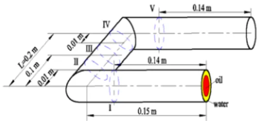
Fig. 1. Geometry of computational domain.
3.
N
UMERICAL SOLUTION3.1
Construction of Geometry and Mesh
Distribution
For this study, the computational geometry (∏ -bend) is shown in Fig. 1. The geometry consists of a tube of 0.012m diameter (D), and the initial
distance (L) between the two arms is 0.2m. The aspect ratio (L/D) is 16.67, and the length of arm is 0.15m which was found adequate to achieve fully developed core annular flow before flow across two rectangle elbows. In order to form the core annular flow, co-axial entry of both the liquids with oil (Newtonian or non-Newtonian oil) at the center, and water at the annular surface has been considered. For plotting the velocity, pressure and phase volume fraction distribution along the length of ∏-bend, five cross-sections are established (cross-section I-V in Fig. 1).
The computational geometry is meshed with hexahedral cell by using ANSYS Workbench 14.5. The total number of volume cells for ∏-bend model is 81164 (see Fig. 2) which has been selected by balancing the available computational capability with the achieved accuracy of the solution. In order to ensure the mesh independence of the results, adequate checks have been performed, and the average of oil volume fraction with different cell number are shown in Fig. 3. It has been noted that the results are independent of the cells for the present set of cells.
Fig. 2. The meshed geometry.
Fig. 3. The comparison of average of oil volume fraction under different cells number. vso=0.4-0.6
Table 1 Physical properties of non-Newtonian oil
Oil name Density (kg/m3)
Fluid consistency
coefficient
Flow behavior
index
Surface tension (N/m)
CMC1 (Xu, 2010) 999.9 0.089 0.789 0.0714
CMC2 (Xu, 2010) 1000.0 0.469 0.658 0.0718
CMC3 (Xu, 2010) 1000.4 0.972 0.615 0.0727
CMC4 (Maiumder et al., 2007) 1000.8 0.00218 0.948 0.0735 CMC5 (Maiumder et al., 2007) 1001.2 0.00419 0.910 0.0745 CMC6 (Maiumder et al., 2007) 1001.3 0.00588 0.871 0.075 CMC7 (Maiumder et al., 2007) 1001.5 0.00692 0.850 0.0755
3.2
Solution Strategy and Convergence
Criterion
Flow modeling and the post processing for this CFD study have been conducted in FLUENT 14.5 which is commercial CFD software. Owing to the dynamic behavior of two-phase flow, an unsteady state simulation with a time step of 0.0001s is taken for computation. The independent test of time step size has been conducted, and the results are shown in Fig. 4. This figure confirms the average oil volume fraction does not change much when time step size is decreased from 0.0005s to 0.00005s. Different methods of discretization of the governing equations are used. Continuity equation has been discretized by PRESTO scheme. Momentum is discretized by first order upwind method (the different between the first order upwind scheme and the second order upwind is less than 6%, see Fig. 4, but the first order upwind is quickly than that in this case). To pressure velocity coupling, PISO algorithm is used.
Fig. 4. The comparison of average of oil volume fraction under different time step size and discretized scheme. vso=0.4-0.6 m/s and vsw
=0.6-1.0 m/s, downflow.
The convergence criteria are based on the residual value of the computed variables namely mass, velocity components and volume fraction. In this analysis, the numerical calculation is considered converged when the residuals of the different variables are lowered by three orders of magnitude.
3.3 Boundary
Condition
and Fluid Material Appropriate inlet and boundary conditions are significant for a successful simulation ofhydrodynamics behavior in the ∏-bend. At the oil inlet, oil superficial velocity (vso) and oil phase
volume fraction (o=1) are set. At the water inlet, water superficial velocity (vsw) and water phase
volume fraction (w=1) are set. At the outlet, pressure outlet boundary is used and the diffusion flux for the variables in exit direction is set to zero. In addition, the wall of bend is imposed with no-slip, no penetration boundary condition. The contact angle between water and pipe material is also specified at the wall.
In this simulation, seven non-Newtonian oils are utilized, which properties are shown Table 1.
4.
R
ESULTS AND DISCUSSION4.1
Comparison with Experiment and
Empirical Correlation
The numerical simulation is validated against experiment of Sharma et al. (2011), which is Newtonian oil (lube oil, =960 kg/m3, =0.2
Pa.s, =0.039 N/m) and water core annular flow through the ∏-bend. The comparison of simulated and experimental result is shown in Fig. 5a. From Fig. 5a, it is clear that the simulated result appears reasonably consistent with the experimental observation. Fig. 5b presents the predicted oil phase volume fraction (o) for four different input water fraction, which are very close compared with the empirical formula (6) (the error between the numerical and experimental results is less than 5%). For Fig. 5, it signifies that the VOF model combined with the CSS model could capture the physics phenomena of a oil-water core annular flow.
4.2
Hydrodynamics of Core Annular flow
After validation with experiment and empirical correlation, the model is directed to generated information regarding the phase fraction, the total pressure and the velocity distribution during a core annular downflow through the ∏-bend.At first, the oil phase volume fraction contour and radial profile at five different axial locations of the
velocity, vsw=0.15 m/s (the oil is CMC1, the
sections I-V are in Fig. 1, as downflow, cross-section V is the upstream and cross-cross-section I is downstream). It is clear that core flow at the mid-section is eccentric in nature, and also reveals the three-dimension nature of the interfacial configuration. Fig. 6b depicts the radial profiles of oil phase fraction at five different axial locations, it shows that the oil holdup has its maximum value at left side of the location I and IV, while its maximum value is at center of the other positions.
Fig. 5. Comparison with experiment and empirical correlation. a) numerical and experimental contour during core annular downflow through the ∏-bend; oil, water. b) numerical results and empirical correlation. vso=0.4-0.6 m/s and vsw=0.6-1.0 m/s, downflow.
Furthermore, the heavier CMC1 oil tries to occupy the downside of the tube during its downflow at the upstream and downstream because of its gravity. And at the cross-section III of ∏-bend, the oil phase occupies the left side, due to the centrifugal forces. At the cross-section I and IV, the oil core is evident to lean one side, because the oil-water flow direction is suddenly changed (see Fig. 7).
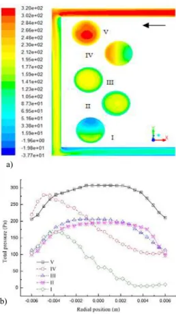
Fig. 6. Oil phase volume fraction contours and radial profiles. a) oil phase volume fraction contour; b) radial profiles of oil phase volume fraction at different cross-section. vso=0.15 m/s
and vsw=0.15 m/s, downflow.
Fig. 7. Pressure contours and radial profiles. a) total pressure contour; b) pressure radial profiles at different cross-section. vso=0.15 m/s
and vsw=0.15 m/s, downflow.
Next the total pressure contours and radial profiles at five different axial locations are shown in Fig. 7. Fig. 7a shows the total pressure contours in longitudinal and cross sections, and it is evident that the total pressure decreases gradually as the flow from upstream towards downstream. For better understanding the phenomenon, Fig. 7b shows the radial variation of total pressure at five different cross-sections. There is not much variation of pressure at the cross-section II, III, and V, while there is a distinct change in the slope at the cross-a)
b)
a)
b)
a)
section I and IV, that is, the total pressure is found to have its maximum value close to one side wall at cross-section I and IV, however, at the cross-section II, III and V, the maximum value of the total pressure is located on the center of pipe.
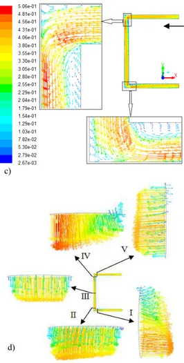
In order to understand the variation of velocity in the return bend, Fig. 8 depicts the velocity contours and radial profiles of velocity at different sections. Fig. 8a represents the velocity contour of longitudinal and cross sections, it can be seen that velocity is higher at the center and gradually decreases to zero at the wall, and increases as two-phase flow moves towards the outlet. Fig. 8b shows the velocity profiles at five different cross-sections, it is clear that the velocity profiles are flat at the cross-section II, III and V, while they assumes a crest curve at the cross-section I and IV. This velocity profiles changing leads to a variation of the phase distribution and the total pressure distribution before-mentioned. For better understanding the velocity field, the velocity vector is illustrated in Fig. 8c. From Fig. 8c, at the two right angle corners of ∏-bend, Two phase flow on the outer wall and separation at the inner wall make flow very complicated, the flow velocity increases from the inner wall to the outer wall, and a very prominent vortex zone is observed owing to suddenly changed flow direction. Fig. 8d depicts the velocity vectors at the five cross-sections, it can be clear observed that the vectors direction don’t keep consistent, there is reverse flow near wall of the cross-section I, IV and V, and it shows that the velocity magnitude of flow on the wall is also zero.
Fig. 8. Velocity contours, radial profiles and vector. a) velocity magnitude contour; b) velocity
radial profiles at different cross-section; c) velocity vector of longitudinal section; d) velocity
vector of cross-sections. vso=0.15 m/s and
vsw=0.15 m/s, downflow.
4.3
Effect of Oil Properties on Core Flow
Further studies have been directed to understand the variation of total pressure gradient (k) and maximum wall shear stress with different non-Newtonian oil properties. Fig. 9 depicts the variation of total pressure gradient (k) and maximum wall shear stress with oil properties (see Table 1) for downflow with vso=0.15 m/s andvsw=0.15 m/s. It can be observed from this figure
that different oil properties differ in their flow behavior. The pressure gradient increases with an increase of oil density and fluid consistency coefficient (K), and a decrease of flow behavior index (n) (these results give a good agreement with the data of Das et al.(1991)). The reason behind this is that an increase in oil density and fluid consistency coefficient, increases the gravity and centrifugal force, as a result the total pressure gradient increases. Similar behavior is also valid for maximum wall shear stress.
The contours of non-Newtonian oil volume fraction with different oil properties are shown in Fig. 10 (oil volume fraction of CMC1 is shown in Fig. 6a). b)
c)
d)
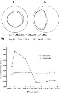
In this simulation, seven non-Newtonian oils (see Table1) can be classified as high consistency or low consistency oil, depending on their fluid consistency coefficient (K). From CMC1 to CMC3, is high consistency oil, while CMC4 to CMC7 is low consistency oil. From Fig. 10a and Fig. 6a, they have some similar contours under the developed core annular flow through ∏-bend. However, the interfaces between oil and water have significant difference in the two right angle corners. As the oil density increases, the oil core is easy to touch the pipe wall (see oil phase distribution on the cross-section I in the Fig. 10a). Fig. 10b and 10c compare the oil core shape and area-weighted average of the oil phase volume fraction at the cross-section II and IV, it can be seen that the oil core shape and oil area-weighted average are influenced by the oil properties. In Fig. 10b, the left position of the oil core shape is nearly same, but the right position is varied according to the oil properties. From Fig. 10c, the oil volume fraction varies by quantitatively display, as increasing of the density and the consistency coefficient (K), decreasing of the flow behavior index (n), the oil volume fraction at the two cross-section increases first, and then decreases, it attain the minimum value, then increases slightly. These phenomena are because of coupling action of gravity and centrifugal force induced by their different properties .
Fig. 9. Variation of total pressure gradient and maximum wall shear stress with the
non-Newtonian oil properties.
Fig. 10. Oil phase volume fraction with different oil properties. a) comparison of phase volume fraction distribution on the cross-section I, III, and V; b) comparison of oil core shape on the cross-section II and IV; c) area-weighted average
of the oil phase volume fraction on the cross-section II and IV.
In order to understand the difference between non-Newtonian oil-water flow and non-Newtonian oil-water flow inside of the return bend, comparisons of the total pressure and velocity distribution are shown in Fig. 11. Fig. 11a represents the total pressure profiles at cross-section I and V during full development of core annular flow with two type oils. It can be easily noticed that the total pressure of Newtonian oil-water flow is higher than that of non-Newtonian oil-water flow at the upstream (cross-section V), and they have little difference at the downstream (cross-section I). Fig. 11b illustrates the velocity profile at two corresponding cross-sections. The velocity of non-Newtonian water flow is higher than that of Newtonian oil-water flow at the upstream, and at downstream, they have similar distribution. This figure also shows that the distribution of total pressure and velocity magitude of two type oils have similar disrtibution trend.
4.4
Effect of flow Direction on Core flow
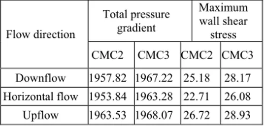
Attempts have next been conducted to investigate the effect of flow direction on flow field. The up, down and horizontal core flow across ∏-bend at vso=0.15 m/s and vsw=0.3 m/s are simulated. Table 2shows the flow directions influence on the total pressure gradient and wall shear stress, it is noted that the total pressure gradient and maximum wall shear stress of upflow is greatest among three flow direction, so this flow direction should be avoid in
b)
c)
the applications. Fig. 12 shows that the oil phase (CMC2) distribution inside the pipe with the different flow directions, it clearly illustrates the oil core may easily impact the pipe wall in the two right corner as in the upflow.
Fig. 11. Flow parameters comparison of Newtonian oil and non-Newtonian oil. a) comparison of total pressure distribution b) comparison of velocity magnitude. vso=0.15
m/s and vsw=0.15 m/s, downflow.
Table 2 Total pressure gradient and maximum wall shear stress with different flow direction.
Flow direction
Total pressure gradient
Maximum wall shear stress
CMC2 CMC3 CMC2 CMC3
Downflow 1957.82 1967.22 25.18 28.17
Horizontal flow 1953.84 1963.28 22.71 26.08
Upflow 1963.53 1968.07 26.72 28.93
4.5
Effect of Geometry Parameters on
Core flow
Subsequently, attempts have been made to understand the influence of bend parameters on flow field. For this study, the aspect ratio (length to diameter of bend, L/D) is varied from 6.25 to 31.25. Fig. 13 represents the variation of total pressure gradient and maximum wall shear stress with L/D for constant oil and water superficial velocity (vso=0.15 m/s and vsw=0.15 m/s, downflow). It is
evident from the figure that total pressure gradient decreases sharply with increases in L/D (<12.5) and
then declines slowly. The maximum wall shear stress decreases firstly and then increases with the increasing aspect ratio. Because as L/D increases, it leads to the potential between two cross-section of oil-water two-phase flow increase, and then the total pressure difference of two section decreases. Combined the curvature lines of total pressure gradient and maximum wall shear stress, the aspect ratio is at range of 14 to 21 is preferable for non-Newtonian oil and water core annular flow through the ∏-bend.
Fig. 12. Oil phase distribution comparison of different flow directions.
Fig. 13. Total pressure gradient and maximum wall shear stress as a function of L/D.
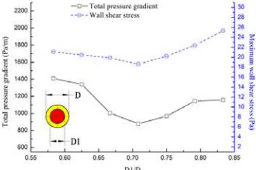
To investigate the effect of inlet diameter ratio (inlet oil diameter D1 to pipe diameter D, D1/D) on total pressure gradient and maximum wall shear stress, the inlet diameter ratio is varied from 0.583 to 0.833. The variation of total pressure gradient and maximum wall shear stress with D1/D is depicted in Fig. 14. It has been observed that a decrease in the total pressure gradient with increases in the D1/D, and after D1/D=0.71 the total pressure gradient increase. For the maximum wall shear stress, it also decreases gradually until it attains a minimum and then increases with increasing D1/D. The reason is that as D1/D increases, the volume fraction of oil increases, thus leads to the oil velocity reduces with keeping the a)
same superficial velocity, and then the total pressure gradient decreases. However, when the D1/D increases continuously, the water film decreases sharply, and its velocity increases quickly, thus leads to the total pressure gradient increases. From the total pressure gradient and maximum wall shear stress point of consideration for a given operating condition, the inlet diameter ratio ranging from 0.667 to 0.79 is suitable to keep the lower total pressure gradient and shear stress in the ∏-bend.
Fig. 14. Total pressure gradient and maximum wall shear stress as a function of D1/D.
Further, to understand the effect of the fillet radius ratio (by rounding of right angle elbow, is defined with R/D, R is the fillet radius) on the total pressure gradient and maximum wall shear stress, the models with different R/D for given superficial oil and water velocity (vso=0.15 m/s and vsw=0.15 m/s) downflow
are calculated. Fig. 15 represents the influence of R/D on the total pressure gradient and maximum wall shear stress. The total pressure gradient decreases continually with increasing R/D, while the maximum wall shear stress increases until it attains a maximum and then decrease sharply with an increase of R/D. The reason behind this can be explained that the frictional resistance decreases with an increase of R/D, thus leads to the total pressure difference of two cross-sections decrease. Fig. 16 depicts the velocity vector and interface between non-Newtonian oil and water in the rounding ∏-bend. It is evident from this figure that the recirculatory domain occurred in Fig. 8 are disappeared, and flow is more stable. The figures also denotes in case of R/D>2.5, the total pressure gradient and maximum wall shear stress can be kept lower value, and thus is significant to reduce pumping power.
Fig. 15. Total pressure gradient and maximum wall shear stress as a function of R/D.
Fig. 16. Vector and interface of non-Newtonian oil and water flow in the rounding ∏-bend.
5.
C
ONCLUSIONSIn the present study, the laminar core annular flow of non-Newtonian oil and water across ∏-bend is investigated. For simulated with Newtonian oil by using CFD software FLUENT 14.5, the tendency of phase distribution contour agrees well with the results of experimental observation (Sharma et al., 2011), and the oil phase volume fraction is good agreement with the empirical formula. From the study the following conclusions can be made:
(1) The VOF and CSS models can give a satisfactory predication of the interfacial structures, pressure, velocity, and wall shear stress distributions.
(2) The non-Newtonian oil properties do influence on the non-Newtonian oil water core annular flow through ∏-bend. The variation of the pressure gradient and wall shear stress relates to the oil density, fluid consistency coefficient (K), and flow behavior index (n), this is because of coupling action of gravity and centrifugal force.
(3) The flow direction has little effect on the total pressure gradient and wall shear stress, however the total pressure gradient and wall shear stress have the maximum value as oil-water flow is upflow.
(4) The effects of aspect ratio, inlet diameter ratio and fillet radius ratio on the hydrodynamics parameters are analyzed, and the results show that the aspect ratio ranging from 14 to 21, the inlet diameter ratio ranging from 0.667 to 0.75, and the fillet radius ratio greater 2.5 the non-Newtonian oil-water two-phase may experience a more stable core annular flow through the ∏-bend. At same time, the filleted right angle elbow of ∏-bend should improve the flow status, and reduce the pressure gradient and wall shear stress.
A
CKNOWLEDGEMENTSin Guangzhou (2012A084), Science and Technology Plan Project of Guangdong Province (2012B061000013), Popular Science Project of Guangzhou (2013KP042) and Open Fund of Key Laboratory of Innovation Method and Decision Management System of Guangdong Province (2011A060901001-19D).
R
EFERENCESArney, M. S., R. Bai , E. Guevara, D. D. Joseph and K. Liu (1993). Friction factor and holdup studies for lubricated pipeline-I: Experiments and correlations. Int. J. Multiphase Flow 19, 1061-1076.
Bai, R., K. Chen and D. D. Joseph (1992). Lubricated pipelining: stability of core-annular flow: part 5. Experiments and comparison with theory. J. Fluid Mech. 19, 97-132.
Bai, T., K. Kelkar and D. D. Joseph (1996). Direct simulation of interfacial waves in a high viscosity ratio and axisymmetric core annular flow. J. Fluid Mech. 327, 1-34.
Bandyopadyay, T. K. and S. K. Das (2007). Non-Newtonian pseudoplastic liquid flow through small diameter piping components. J. Petrol. Sci. Eng. 55, 156-166.
Bandyopadyay, T. K. and S. K. Das (2013). Non-Newtonian and Gas-non-Non-Newtonian liquid flow through elbows – CFD analysis. J. Applied Fluid Mech. 6, 131-141.
Banerjee, T. K., M. Das and S. K. Das (1994). Non-Newtonian liquid flow through globe and gate valves. Can. J. Chem. Eng. 72, 207-211.
Blyth, M. G. and A. P. Bassom (2013). Stability of surfactant-laden core-annular flow and rod-annular flow to non-axisymmetric modes. J. Fluid Mech. 716, R13.
Brauner, N. (1991). Two-phase liquid-liquid annular flow. Int. J. Multiphase Flow 17, 59-76.
Chen, I. Y., Y. S. Wu , J. S. Liaw and C. C. Wang (2008). Two-phase frictional pressure droop measurements in U-type wavy tubes subject to horizontal and vertical arrangements. Appl. Therm. Eng. 28(8-9), 847-855.
Chen, I. Y., Y. W. Yang and C. C. Wang, (2002). Influence of horizontal return bend on the two-phase flow pattern in 6.9mm diameter tubes. Can. J. Chem. Eng. 82, 478-484.
Cruz, D. A., P. M. Coelho and M. A. Alves (2012). A simplified method for calculating heat transfer coefficients and friction factors in laminar pipe flow of non-Newtonian fluids. J. Heat Transfer 134, 091703.
Das, S. K., M. N. Biswas and A. K. Mitra (1991). Non-Newtonian liquid flow in bends. Chem. Eng. J. 45, 165-171.
Dong, X. H., H. Q. Liu, Q. Wang, Z. X. Pang and C. J. Wang (2013). Non-Newtonian flow characterization of heavy crude oil in porous media. J. Petrol. Explore Prod. Tech. 3, 43-53.
Edwards, M. F., M. S. M. Jadallah and R. Smith (1985). Head losses in pipe fittings at low Reynolds numbers. Chem. Eng. Res. Design 63, 43-50.
Jiang, F., Y. J. Wang, J. J. Ou and Z. M. Xiao (2014). Numerical simulation on oil-water annular flow through the Π bend. Ind. Eng. Chem. Res. 53, 8235-8244.
Jiang, F., Y. J. Wang, J. J. Ou and C .G. Chen (2014). Numerical simulation of oil-water core annular flow in a U-bend based on the Eulerian model. Chem. Eng. Tech. 37, 659-666.
Kerpel, K. D., B. Ameel, H. Huisseune, C. T’Joen, H. Caniere and M. D. Paepe (2012). Two-phase flow behavior and pressure drop of R134a in a smooth hairpin. Int. J. Heat Mass Transfer 55,1179-1188.
Ko, T., H. G. Choi, R. Bai and D. D. Joseph (2002). Finite element method simulation of turbulent wavy core-annular flows using a k-w turbulence model method. Int. J. Multiphase Flow 28, 1205-1222.
Lafaurie B., C. Nardone, R. Scardovelli, S. Zaleski and G. Zanetti (1994). Modeling merging and fragmentation in multiphase flows with SURFER. J. Comp. Phys. 113, 134-147.
Lennon O. N. and D. M. S. Peter (2010). Interfacial instability of turbulent two-phase stratified flow: Pressure-driven flow and non-Newtonian layers. J. Non-Newtonian Fluid Mech. 165, 489-508.
Li H. W., T. N. Wong, M. Skote and F. Duan (2013). A simple model for predicting the pressure drop and film thickness of non-Newtonian annular flows in horizontal pipes. Chem. Eng. Sci. 102, 121-128.
Li, J. and Y. Renardy (1999). Direct simulation of unsteady axisymmetric core-annular flow with high viscosity ratio. J. Fluid Mech. 391, 123-149.
Maiumder, S. K., G. Kundu and D. Mukheriee (2007). Pressure drop and bubble-liquid interfacial shear stress in a modified gas non-Newtonian liquid downflow bubble column. Chem. Eng. Sci. 62, 2482-2490.
Duijvestijn (1987). Core annular oil/water flow: the turbulent-lubricating-film model and measurements in a 5 cm pipe loop. Int. J. Multiphase Flow 13, 23-31.
Ooms, G., M. J. B. M. Pourquie and J. C. Beerens (2013). On the levitation force in horizontal core-annular flow with a large viscosity ratio and small density ratio. Phys. Fluids 25, 032102.
Ooms, G., A. Seoal, A. J. Vanderwees, R. Meerhoff and R. V. A. Oliemans (1984). A theoretical model for core-annular flow of a very viscous oil core and a water annulus through a horizontal pipe. Int. J. Multiphase Flow 10, 41-60.
Ooms, G., C. Vuik and P. Poesio (2007). Core-annular flow through a horizontal pipe: Hydrodynamic counterbalancing of buoyancy force on core. Phys. Fluid 19, 092103.
Padilla, M., R. Revellin, J. Wallet and J. Bonjour (2013). Flow regime visualization and pressure drops of HFO-1234yf, R-134a and R-410A dring downward two-phase flow in vertical return bends. Int. J. Heat Fluid Flow 40, 116-134.
Prada, J. W. V. and A. C. Bannwart (2001). Modeling of vertical core-annular flows and application to heavy oil production. J. Eng. Resource Tech. 123, 194-199.
Rodriguez, O. M. H. and R. V. A. Oliemans (2006). Experimental study on oil-water flow in horizontal and slightly inclined pipes. Int. J. Multiphase Flow 32:323-343.
Rodriguez, O. M. H., A. C. Bannwart and C. H. M. Carvalho (2009). Pressure loss in core-annular flow: Modeling, experimental investigation and full-scale experiments. J. Petrol. Sci. Eng. 65, 67-75.
Russell, T. W. F. and M. E. Charles (1959). The effect of less viscous liquid in the laminar flow of two immiscible liquids. Can. J. Chem. Eng.
37, 18-24.
Sharma, M., P. Ravi, S. Ghosh, G. Das and P. K. Das (2011). Hydrodynamics of lube oil-water flow through 180°returen bends. Chem. Eng. Sci. 66, 4468-4476.
Sotgia, G., P. Tartarini and E. Stalio (2008). Experimental analysis of flow regimes and pressure drop reduction in oil-water mixtures. Int. J. Multiphase Flow 34,1161-1174. Srivastava, R. P. S. (1977). Liquid film thickness in
annular flow. Chem. Eng. Sci. 28, 819-824.
Strazza, D., B. Grassi, M. Demori, V. Ferrari and P. Poesio (2011). Core-annular flow in horizontal and slightly inclined pipes: Existence, pressure drops, and hold-up. Chem. Eng. Sci. 66, 2853-2863.
Strazza, D. and P. Poesio (2012). Experimental study on the restart of core-annular flow. Chem. Eng. Res. Design 90, 1711-1718. Turian, R. M., T. W. Ma, F. L. G. Hsu, M. D. J.
Sung and G. W. Plackmann (1998). Flow of concentrated non-Newtonian slurries: 2. Friction losses in bends, fittings, valves and venture meters. J. Multiphase Flow 24, 243-269.
Usui, K., S. Aoki and A. Inoue (1980). Flow behavior and pressure drop of two-phase flow through C-shaped bend in vertical plane, (I) upward flow. J. Nuclear Sci. Tech. 17, 875-887.
Wang, C. C., I. Y. Chen and P. S. Huang (2005). Two-phase slug flow across small diameter tubes with the presence of vertical return bend, Technical Note. Int. J. Heat and Mass Transfer 48, 2342-2346.