The Cryosphere, 7, 205–216, 2013 www.the-cryosphere.net/7/205/2013/ doi:10.5194/tc-7-205-2013
© Author(s) 2013. CC Attribution 3.0 License.
Geoscientiic
Geoscientiic
Geoscientiic
The Cryosphere
Open Access
Analysis of the snow-atmosphere energy balance during wet-snow
instabilities and implications for avalanche prediction
C. Mitterer and J. Schweizer
WSL Institute for Snow and Avalanche Research SLF, Davos Dorf, Switzerland
Correspondence to:C. Mitterer ([email protected])
Received: 14 June 2012 – Published in The Cryosphere Discuss.: 23 July 2012
Revised: 7 December 2012 – Accepted: 28 December 2012 – Published: 1 February 2013
Abstract.Wet-snow avalanches are notoriously difficult to
predict; their formation mechanism is poorly understood since in situ measurements representing the thermal and me-chanical evolution are difficult to perform. Instead, air tem-perature is commonly used as a predictor variable for days with high wet-snow avalanche danger – often with limited success. As melt water is a major driver of wet-snow insta-bility and snow melt depends on the energy input into the snow cover, we computed the energy balance for predict-ing periods with high wet-snow avalanche activity. The en-ergy balance was partly measured and partly modelled for virtual slopes at different elevations for the aspects south and north using the 1-D snow cover model SNOWPACK. We used measured meteorological variables and computed energy balance and its components to compare wet-snow avalanche days to non-avalanche days for four consecutive winter seasons in the surroundings of Davos, Switzerland. Air temperature, the net shortwave radiation and the energy input integrated over 3 or 5 days showed best results in dis-criminating event from non-event days. Multivariate statis-tics, however, revealed that for better predicting avalanche days, information on the cold content of the snowpack is nec-essary. Wet-snow avalanche activity was closely related to periods when large parts of the snowpack reached an isother-mal state (0◦C) and energy input exceeded a maximum value of 200 kJ m−2in one day, or the 3-day sum of positive energy
input was larger than 1.2 MJ m−2. Prediction accuracy with
measured meteorological variables was as good as with com-puted energy balance parameters, but simulated energy bal-ance variables accounted better for different aspects, slopes and elevations than meteorological data.
1 Introduction
Wet-snow avalanches are difficult to forecast, but often threaten communication lines in snow-covered mountain ar-eas. Once the snowpack becomes wet the release probabil-ity obviously increases, but determining the peak and end of a period of high wet-snow avalanche activity is particularly difficult (Techel and Pielmeier, 2009).
Processes leading to wet-snow avalanches are complex and the conditions of the snowpack may change from sta-ble to unstasta-ble in the range of hours (Trautman, 2008). The presence of liquid water within the snowpack in the starting zone is a prerequisite and several field campaigns (Brun and Rey, 1987; Bhutiyani, 1996) and experiments under labora-tory conditions (Zwimpfer, 2011; Yamanoi and Endo, 2002) found decreasing shear strength with increasing liquid wa-ter content. However, quantifying the amount of liquid wawa-ter within the snowpack is a difficult task as even experienced observers tend to overestimate the amount of liquid water (Fierz and F¨ohn, 1995; Techel and Pielmeier, 2011). Only objective measurement devices relating the relative permit-tivity of the 3-phase medium wet snow to an amount of water provide reliable results. Most devices though are for research purposes only and until today the operational use is hindered by practical and financial constraints. In addition, no estab-lished procedure exists to assess wet-snow instability. In situ stability tests commonly used to assess dry-snow instability showed ambiguous results when performed in moist or wet-snow covers (Techel and Pielmeier, 2010).
sum of precipitation is the strongest forecasting parameter (Schweizer et al., 2009) and closely related to avalanche dan-ger (Schweizer et al., 2003a), air temperature is often used as a critical parameter for predicting wet-snow avalanche activ-ity (McClung and Schaerer, 2006). It is included in statis-tical prediction tools that were designed for a specific area (e.g. Romig et al., 2005). However, there are many examples which show that air temperature is in many cases not a good predictor and causes a high number of false alarms (Kattel-mann, 1985). Nevertheless, it appears to be a variable clearly related to wet-snow instability (Baggi and Schweizer, 2009; Peitzsch et al., 2012).
To clarify the meteorological boundary conditions favour-ing the triggerfavour-ing of wet-snow avalanches, we analyzed four winter seasons (from 2007–2008 to 2010–2011) with differ-ent distinct wet-snow avalanche evdiffer-ents in the surroundings of Davos, Switzerland. As suggested by Trautman (2008), we computed the entire energy balance for the snowpack with special attention to the main sources for snow melt, namely the incoming longwave and shortwave radiation and the sen-sible heat flux (Ohmura, 2001). We used univariate and mul-tivariate statistics to evaluate whether these three sources were relevant shortly before and during the instabilities. In addition, we analyzed meteorological parameters of nearby stations and evaluated whether the predictive power of the energy balance and its terms performed better than widely used meteorological parameters such as air temperature.
2 Data
2.1 Avalanche occurrence
Avalanche occurrence data were recorded for the winters 2007–2008 to 2010–2011 for the surroundings of Davos, Switzerland. Data consisted of avalanche size (Canadian avalanche size class, McClung and Schaerer, 2006) and included only events which were classified as wet-snow avalanches. The classification into wet or dry is based on observation, mainly on visual clues. No measurements on the amount of liquid water within the starting zones were available but most observers are well trained to discrimi-nate between wet and dry-snow avalanches. We included both, wet-loose avalanches and wet-slab avalanches in our avalanche days. Considering all avalanche cycles, about as many loose-snow avalanches as slab avalanches were re-ported (104 vs. 77). With regard to the location of the fail-ure surface, 42 % released within the snowpack and 58 % of the avalanches at the snow–soil interface. We calculated a daily avalanche activity index (AAI) using a weighted sum of recorded avalanches per day with weights of 0.01, 0.1, 1 and 10 for size classes 1 to 4, respectively (Schweizer et al., 2003b). In order to exclude days with either many small avalanches or with a single large event, only days with an AAI>2 were considered as wet-snow avalanche days for the
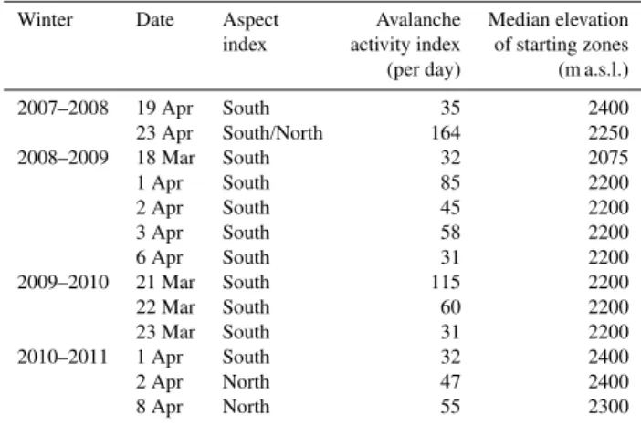
Table 1.Major wet-snow avalanche cycles (i.e. AAI>30) in the surroundings of Davos, Switzerland, for the winters 2007–2008 to 2010–2011. Aspect index was calculated by relating the number and size of avalanches released on slopes of northern to those on south-ern aspects. Only for the cycle on 23 April 2008 no clear aspect could be assigned. Days with low activity are not included in the Table.
Winter Date Aspect Avalanche Median elevation index activity index of starting zones (per day) (m a.s.l.) 2007–2008 19 Apr South 35 2400 23 Apr South/North 164 2250 2008–2009 18 Mar South 32 2075 1 Apr South 85 2200 2 Apr South 45 2200 3 Apr South 58 2200 6 Apr South 31 2200 2009–2010 21 Mar South 115 2200 22 Mar South 60 2200 23 Mar South 31 2200 2010–2011 1 Apr South 32 2400 2 Apr North 47 2400 8 Apr North 55 2300
statistical analyses (see below). In addition, we calculated the median elevation of the release zones. Due to the recording system used in Switzerland it was not possible to relate sin-gle events and their size to a given aspect as one record may contain multiple events – still the dominating aspects are re-ported. Therefore, we introduced an aspect index, which is the ratio of the frequency and size of avalanches recorded in southern aspects to the one recorded in northern aspects. If the ratio was>1 we assumed that the avalanche cycle mainly occurred in southern aspects and vice versa for<1. Follow-ing this approach, we obtained 66 wet-snow avalanche days and 663 non-avalanche days for the four winters. The ma-jor avalanche cycles with date, aspect index and elevation of release zones are given in Table 1.
2.2 Meteorological data
Meteorological data were obtained from three automatic weather stations: Weissfluhjoch (WFJ, 2540 m a.s.l.), Still-berg (STB, 2150 m) and DorfStill-berg (DFB, 2140 m). After the first winter season 2007–2008 data from STB were replaced by data from the new Dorfberg weather station, which is lo-cated in the vicinity of a well-known wet-snow avalanche starting zone. The three stations are located at two distinct el-evations: STB and DFB are slightly above the tree-line, near the lower limit of where most wet-slab avalanches are initi-ated, and WFJ is located higher than most starting zones of all wet-snow avalanche cycles.
2.3 Simulations with SNOWPACK
In order to obtain energy balance data for slopes of various elevations and aspects we used the 1-D snow cover model SNOWPACK (Lehning et al., 2002a, b; Lehning and Fierz, 2008). Slope angle was fixed to 35◦ which represents the median slope angle of all recorded wet-snow avalanche re-leases. Input data for the model were meteorological values taken only from the weather station Weissfluhjoch (WFJ); we had to extrapolate or adapt air temperature, snow sur-face temperature and incoming shortwave radiation for dif-ferent elevations and aspects. Air temperature was extrapo-lated using a constant lapse rate of 0.65◦C/100 m. Outgoing longwave radiation and consequently snow surface tempera-ture was modelled in SNOWPACK using Neumann bound-ary conditions (Lehning et al., 2002b). We adapted the input of the shortwave radiation according to the lapse rate sug-gested by Marty (2001) which is a lapse rate based on mea-surements at different elevations. We did simulations only for slopes of the two main aspects, i.e. 0◦(N) and 180◦(S). The change in incoming solar radiation on these aspects was taken into account. In brief, to run the model, we used air temperature, relative humidity, incoming shortwave, incom-ing longwave, reflected shortwave radiation, wind direction, wind speed, and snow depth. Components of the radiation balance and air temperature including relative humidity were measured under ventilated conditions. Simulations were per-formed for 2000, 2200 and 2500 m a.s.l. For slope simula-tions, snow depth was modelled with a precipitation mass input and albedo was determined as a function of grain type, grain size and presence of liquid water at the snow surface. Again daily means, maximum, minimum and 1, 3 and 5 day sums were derived from the energy balance terms.
3 Methods
3.1 Calculation of energy balance and liquid water
The energy balance was calculated using SNOWPACK. Within the model the energy balance can be calculated in two different ways. The first mode calculates the net change rate dH/dtof the snowpack’s internal energy per unit area as the sum of all energy fluxes at the surface:
−dH dt =S
↓+S↑+L↓+L↑+H
S+HL+HP+G, (1)
whereS↓ andS↑ are the downward and reflected compo-nents of shortwave radiation, respectively,L↓andL↑are the downward and upward components of longwave radiation, respectively,HS andHLare the turbulent fluxes of sensible
and latent heat through the atmosphere,HPis the flux of
en-ergy carried as sensible or latent heat by both precipitation and blowing snow, andGis the ground heat flux (King et al., 2008).
For our analysesS↓,S↑,L↓andL↑were measured,HS, HLandHP modelled, andGfixed to a constant value. The
sensible heatHS(Eq. 2) and the latent heat fluxHL(Eq. 4)
were calculated assuming a neutral atmospheric surface layer and using Monin-Obukhov similarity theory resulting in: HS(0)= −Cρacp(T (z)−T (0)), (2)
whereT (z)is the air temperature at heightz,T (0)the snow surface temperature,ρathe density of air andcpthe heat
ca-pacity; the kinematic transfer coefficientC is given accord-ing to
C= −ku∗ 0.74 lnzz
0
, (3)
wherekis the von Karman constant,u∗is the friction veloc-ity of the wind andzthe height of the wind measurement. The latent heat is defined as
HL= −C
0.622Lw/i RaT (z) [
ews(T (z))RH−esi(T (0))], (4)
whereRa is the gas constant for dry air,Lw/iare the latent
heat values for vaporization and sublimation, respectively, ew/is is the saturation vapour pressure over water or ice, and RH the relative humidity.
Assuming neutral stability conditions are valid during pe-riods with moderate to high wind speeds which often pre-vail in complex mountainous terrain (Lehning et al., 2002a), St¨ossel et al. (2010) showed that outgoing longwave radia-tion is better accounted for within SNOWPACK when forc-ing neutral conditions.
The second mode for the energy balance in SNOWPACK involves calculating the internal change of energy based on either warming and melting, or cooling and freezing; it is given by:
−dH
dt =Lli(RF−RM)−
HS
Z
0
d
dt(ρs(z)cp, iTs(z))
dz, (5)
whereRFandRMare the freezing and melting rate,
respec-tively,Llithe latent heat of fusion of ice, andcp, ithe specific
heat capacity of ice;ρsis the snow density andTsis the snow
SNOWPACK contains parameterisations of water perco-lation, retention and refreezing processes and calculates the liquid water content for single layers. There are two possi-bilities to calculate the liquid water content for every layer within the modelled snow cover (Hirashima et al., 2010). Since water transport, especially on slopes is a very complex phenomenon, the water transport codes that are presently implemented within SNOWPACK cannot depict the full complexity of flowing water within the snowpack which is responsible for wet-snow avalanche formation. Both ap-proaches have benefits, but compared to observations sub-stantial deviations were found (Mitterer et al., 2011). There-fore, we did not use liquid water values calculated for single layers with one of the two schemes in the statistical analy-ses. Instead we used the total amount of liquid water within the snowpack. This value is directly linked to the energy bal-ance and the cold content of snow and gives an estimate of how much water was present during the days with wet-snow avalanche activity.
4 Statistical analyses
The non-parametric Mann–Whitney U-test (Spiegel and Stephens, 1999) was used to contrast meteorological or en-ergy flux variables from avalanche and non-avalanche days. Observed differences were judged to be statistically signif-icant where the level of significance wasp <0.05, i.e. the null hypothesis that the two groups are from the same pop-ulation was rejected. In order to obtain a balanced data set of avalanche and non-avalanche days, we randomly selected the same number of non-avalanche days considering the fre-quency of wet-snow avalanche days per month for the period December–May. Non-avalanche days were selected 10 times and for every run ap-value was computed. We averaged the p-values and only if theU-test indicated a statistically sig-nificant difference, variables were passed to a classification tree analysis (Breiman et al., 1998) and its newer derivative
the RandomForest classification (Breiman, 2001).
Classifi-cation trees were obtained by optimising the misclassifica-tion costs and the complexity (size) of a tree. Tree size was determined through cross-validation (10-fold). To minimise the effect of randomly selecting non-avalanche days, we per-formed the tree analysis 20 times and selected the tree com-bination which showed up in most of the cases (in our case about 2/3).
RandomForest(RF) is a newer derivative of the
classifica-tion tree analysis. We used the package RandomForest (Ver-sion 4.6-2) incorporated in the R-project. The code is based on the work of Breiman (2001). It uses bootstrap samples to construct multiple trees. Each tree is grown with a ran-domised subset of predictors that allows the trees to grow to their maximum size without pruning. Finally the results of all trees are aggregated by averaging the trees. Out-of-bag sam-ples are used to calculate an unbiased error rate and variable
Table 2.Contingency table (total cases:N=a+b+c+d)
Observed
Non-avalanche day Avalanche day Model Non-avalanche day a: correct non-event b: missed event
Avalanche day c: false alarm d: correct event
importance, without the need for a training data set or cross validation. Variable importance is based on how much worse the prediction would be if the data for that predictor were permuted randomly. The stronger the decrease in prediction accuracy, the more important is the variable (Breiman, 2001). As this importance measure is calculated for each node, a
morelocalimportance is given. For our data set we produced
N=500 trees and restricted the randomised subset of pre-dictors to a minimum of 7, but a maximum of √n, where nis the number of predictors passed from the results of the U-test. To assess the performance of the multivariate analysis (classification tree andRandomForest) we used the true skill score (HK), the false alarm ratio (FAR), the probabilities of detection of events (POD), and non-events (PON). With defi-nitions used in contingency tables (Table 2) the measures are defined as follows (Wilks, 1995; Doswell et al., 1990): Probability of detection: POD= d
b+d (6)
Probability of non-events: PON= a
a+c (7)
False alarm ratio FAR= c
c+d (8)
True skill score HK= d b+d −
c
a+c (9)
The true skill score, also called the Hanssen and Kuipers discriminant, is a measure of the forecast success and ac-counts for the correct discrimination of events and non-events. Of course, false-stable predictions can have more serious consequences than false alarms, but too many false alarms will not provide meaningful insight into the meteoro-logical boundary conditions prevailing during wet-snow in-stabilities as we cannot define patterns which are common for unstable wet-snow situations.
5 Results
Table 3.Comparison of avalanche (AvD) to non-avalanche days (nAvD) for meteorological data measured at the weather stations Weiss-fluhjoch (2540 m a.s.l) and Dorfberg (2140 m a.s.l.). Median values are shown; Dorfberg values for the season 2007–2008 are substituted with
values from Stillberg (2150 m a.s.l.). For each variable, distributions from avalanche days and non-avalanche days were contrasted (U-test),
and the level of significance (p-value) is given. Only variables withp <0.05 are shown.
Variable Weissfluhjoch (WFJ) Dorfberg (DFB)
Median p-value Median p-value
AvD nAvD AvD nAvD
TAmean(◦C) −0.4 −4.1 <0.01 3.7 2.6 <0.01
TAmin(◦C) −2.3 −6.7 <0.01 0.5 −6.3 <0.01
TAmax(◦C) 2.1 −1.5 <0.01 5.1 −0.7 <0.01
1TA 3d (◦C) 1.2 −0.1 0.01 1.2 0.1 0.42
63d TA positive (◦C) 65 4 <0.01 357 12 <0.01
65d TA positive (◦C) 97.3 15.7 0.01 520 54 0.01
1HS 3d (cm) −6 0 0.03 −1.5 0 0.36
TSSmean(◦C) −4.2 −6.5 0.01 0 −4.2 0.04
TSSmin(◦C) −10.5 −13.2 0.04 −2.2 −11.6 <0.01
TSSmax(◦C) 0 −1.6 <0.01 0 0 0.19
RHmean(%) 69 78 0.09 72 69 0.03
Min radiation balance (Wm−2) −77 −71 0.02 −72 −70 0.26
Max radiation balance (Wm−2) 110 69 0.04 501 241 0.26
65d positive radiation balance (Wm−2) 3907 3354 0.7 17847 12582 0.49
Mean incoming shortwave (Wm−2) 227 204 0.02 215 173 0.2
Mean outgoing longwave (Wm−2) 301 291 0.02 315 297 0.03
Min outgoing longwave (Wm−2) 277 266 0.03 305 268 <0.01
Max outgoing longwave (Wm−2) 312 304 <0.01 NA NA –
Fig. 1.Contrasting avalanche days (AvD) to non-avalanche days (nAvD) for the daily maximum amount of liquid water within the
snowpack for(a)a subset of non-avalanche days and(b)all
non-event days within the data set with data obtained from a simula-tion representing a south-facing slope. Boxes span the interquartile range, whiskers extend to 1.5 times the interquartile range. Outliers
are shown with open circles. Notches are defined by±1.5 times the
interquartile range divided by the square root of N.
approaches, i.e. classification trees (Figs. 2 and 4) and
Ran-domForest(Fig. 3), and compare the predictive power of the
models created with either meteorological measurements or energy balance variables.
5.1 Univariate analysis
For the meteorological variables minimum, mean, maximum, and the positive sum of air temperature over 3 days, the distri-butions were statistically different withp <0.01 for the two classes of wet-snow avalanche day/non-avalanche day (Ta-ble 3). Therefore, these varia(Ta-bles were significant indicators for a day with an AAI>2. Furthermore, the distributions for the minimum snow surface temperature (TSS) were
signifi-cantly different between the two classes for all stations. The mean and maximum ofTSS, the difference of air temperature
in the last 24 h and the difference in snow height for 24 h or 3 days discriminated between the groups only with the data of WFJ. Not surprisingly, days with an AAI>2 had always higher air and snow surface temperatures and a preceding period (3 or 5 days) with higher air temperatures than non-avalanche days. Also significant differences between the two groups of days were found for some variables derived from the radiation balance measured at the stations. Avalanche days received more energy input through radiation than non-avalanche days, though distributions were not always signif-icantly different; outgoing longwave radiation (L↑) showed always high values for avalanche days. In other words,TSS
Fig. 2. Classification tree to discriminate between avalanche
(AAI>2) and non-avalanche days. Input data were all
meteorolog-ical variables taken from WFJ, ifU-test was significant. Forecast
scores of the tree: probability of detection (POD)=0.89;
probabil-ity of non-events (PON)=0.8; true skill score (HK)=0.69.
The daily minimum of sensible heat (HS), the mean net
longwave, the minimum, mean, maximum value ofL↑, all sums ofL↑ and the 3-day sum of positive energy balance were the only variables for which the differences were judged significant for both aspects (Table 4). All other variables ap-pear only in one of the two aspect classes. For the simulations on south-facing slopes all variables dealing with net and in-coming shortwave radiation (S↓) discriminated well between avalanche and non-event days. Daily minimum and maxi-mum values of the energy balance performed well in dis-tinguishing between avalanche and non-avalanche days for southern slopes only. On wet-snow avalanche days on south-facing slopes, the energy input into the snowpack was higher due to high net shortwave radiation and higher net longwave radiation than on non-avalanche days. Avalanche days on north-facing slopes were characterised by a high minimum value ofHS and long periods (3 days) of energy input.L↑
was always higher on avalanche days than on non-avalanche days.
The maximum value for the total amount of liquid water within the snowpack discriminated well between avalanche and non-avalanche days, but only for southern aspects (Fig. 1a). The difference becomes even more evident when including all available non-avalanche days (Fig. 1b). The interquartile ranges of the two distributions do not overlap at all, however, a considerable number of outliers represent days with a high amount of liquid water, but no avalanche activity. For north-facing slopes the two distributions were similar (Table 4).
Fig. 3.The five most important variables for RandomForest
mod-els built with data obtained from(a)simulated north-facing slopes
(2500 m, 35◦),(b)simulated south-facing slopes (2500 m, 35◦), and
(c)meteorological parameters recorded at the station Weissfluhjoch
to classify wet-snow avalanche and non-avalanche days. Variable importance is based on how much worse the prediction would be if the data for that predictor were permuted randomly; the stronger the decrease in accuracy, the higher is the variable importance.
5.2 Multivariate analysis
For the multivariate approaches we pre-selected the variables based on Table 3 and Table 4 according to their physical meaningfulness and significance in the univariate approach. Again, the same quantity of non-avalanche days (N=66) was selected according to the frequency of avalanche days (N=66) for the months December to May.
The classification tree with the meteorological parameters of WFJ used only terms of the radiation balance to split into the two classes. Air temperature was not chosen by the tree (Fig. 2). Avalanche days were detected with almost 90 % ac-curacy when following the nodes of the tree; non-event days were identified with a probability of 80 %. False-stable pre-dictions were less frequent than false alarms. The
Random-Forest(RF) model with the WFJ data not only included
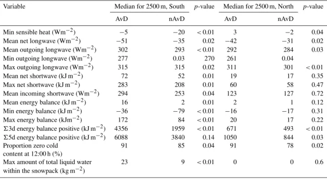
Table 4.Comparison of avalanche (AvD) to non-avalanche days (nAvD) for variables derived from the energy balance calculated for a 35◦
slope. For each variable, distributions from avalanche days and non-avalanche days are contrasted (U-test), and the level of significance
(p-value) is given. Only variables withp <0.05 are shown.
Variable Median for 2500 m, South p-value Median for 2500 m, North p-value
AvD nAvD AvD nAvD
Min sensible heat (Wm−2) −5 −20 <0.01 3 −2 0.04
Mean net longwave (Wm−2) −51 −35 0.02 −42 −31 0.02
Mean outgoing longwave (Wm−2) 302 293 <0.01 292 284 0.03
Min outgoing longwave (Wm−2) 277 0.03 270 261 0.04
Max outgoing longwave (Wm−2) 315 315 0.02 311 301 <0.01
Mean net shortwave (kJ m−2) 72 52 0.01 19 17 0.35
Max net shortwave (kJ m−2) 283 208 0.01 60 58 0.47
Mean incoming shortwave (Wm−2) 294 253 0.04 123 127 0.72
Mean energy balance (kJ m−2) 16 2 0.01 2 1 0.12
Min energy balance (kJ m−2) −36 −79 <0.01 −16 −17 0.31
Max energy balance (kJm−2) 172 84 <0.01 20 17 0.22
63d energy balance positive (kJ m−2) 4356 1959 <0.01 671 493 <0.01
65d energy balance positive (kJ m−2) 6088 3840 0.14 1050 844 0.03
Proportion zero cold 91 85 0.04 91 78 0.02
content at 12:00 h (%)
Max amount of total liquid water 23 9 <0.01 0 0 0.6
within the snowpack (kg m−2)
Fig. 4. Classification tree to discriminate between avalanche
(AAI>2) and non-avalanche days. Input data were all energy
balance variables calculated for a 35◦ south-facing slope at
2500 m a.s.l. Forecast scores of the tree: probability of detection
(POD)=0.84; probability of non-events (PON)=0.83; true skill
score (HK)=0.72.
the DFB data as the univariate analysis did not reveal enough variables (N <7) that discriminated between the two groups of days. The model performance of the DFB tree was worse than the performance of the tree obtained with the WFJ data (Fig. 6). The DFB tree found the events with good accuracy, but produced more false alarms and scored low in detecting non-events.
For a south-facing slope at 2500 m a.s.l., the energy bal-ance summed over 3 days split best followed by the mean net shortwave radiation using classification tree analysis (Fig. 4). The following nodes included the internal state of energy of the snowpack (zero cold content) and the maximum outgoing longwave radiation. For northern slopes (not shown here), again the sum of the energy balance over 3 days split best. The subsequent nodes included sensible heat and the mean of net longwave radiation. Results obtained with
Random-Forests are very similar to those from classification trees,
but variable importance differed. The most important vari-able was the value of zero cold content at noon followed by the mean net shortwave radiation for southern aspects and the mean outgoing longwave radiation for northern aspects. Only then the sum of the positive energy balance values shows up for both aspects (Fig. 3a, b). Again the results obtained with the tree outperform the predictive skills of RF. In none of the multivariate approaches were variables related to the to-tal amount of liquid water chosen.
Fig. 5. (a)Classification tree for WFJ using air temperature
infor-mation,(b)classification tree for air temperature and snow surface
information and(c)for a virtual south-facing slope with energy
bal-ance information only (for predictive skills see Fig. 6).
splitting rules included incoming shortwave radiation and state of the internal energy for south-facing slopes and the sensible and net longwave radiation flux for north-facing slopes. For all cases the predictive skills of the trees were better than the ones of the RF analysis.
5.3 Predictive skills of air temperature and energy
balance
So far results showed that the predictive skills of the two ap-proaches with various input data sets were rather good and mostly agreed. In a next step, however, we wanted to know if either air temperature or the energy balance is sufficient for wet-snow avalanche forecasting and which of both per-forms better. When omitting the radiation terms in the tree presented in Fig. 2, the 5-day sum of positive air temperature remained as the only splitting parameter (Fig. 5a), but model
Fig. 6. Classification accuracy of different tree and RandomFor-est (RF) models for contrasting wet-snow avalanche days to non-avalanche days. Size of the symbols indicates the true skill score.
performance deteriorated (Fig. 6): the tree missed two thirds of all avalanche days, but hardly missed any non-event days. False alarms (0.11) were fairly infrequent. When adding the snow surface temperature (Fig. 5b) the predictive power im-proved (POD=0.89, PON=0.6, FAR=0.3), but the predic-tion accuracy for the non-events went down and the alarm ratio increased. Nevertheless, the number of false-stable predictions was in the same range as with the more complex tree in Fig. 2. Using only information of the en-ergy balance, the tree identified almost all events, but missed many non-events which means that almost two thirds of all non-avalanche days were classified as avalanche days. Intro-ducing the outgoing longwave radiation (not shown here) in-creased the probability of non-events to 90 %, but dein-creased the probability to hit an avalanche day to 67 % (Fig. 6).
6 Discussion
AvD (N) nAvD (N) AvD (S) nAvD (S) 150 200 250 300 350
Mean incoming longw
a
ve r
adiation (W m
− 2) a ● ● ●
AvD (N) nAvD (N) AvD (S) nAvD (S)
150 200 250 300 350
Mean outgoing longw
a
ve r
adiation (W m
− 2) b ● ● ● ● ● ● ● ● ● ● ● ● ●
AvD (N) nAvD (N) AvD (S) nAvD (S)
0 50 100 150
Mean net shor
tw
a
ve r
adiation (W m
−
2) c
● ● ● ● ● ● ● ● ● ● ● ● ● ●
AvD (N) nAvD (N) AvD (S) nAvD (S)
0 100 200 300 400 500
Max net shor
tw
a
ve r
adiation (W m
−
2) d
● ● ● ● ● ● ●
AvD (N) nAvD (N) AvD (S) nAvD (S)
0 20 40 60 80 100 Mean sensib
le heat (W m
− 2) e ● ● ● ● ● ● ● ● ● ● ● ● ● ● ● ● ● ● ● ● ● ● ● ● ● ● ● ● ● ● ● ● ● ● ●
AvD (N) nAvD (N) AvD (S) nAvD (S)
3d sum pos
. energy input (MJ m
− 2) 0 2 4 6 8 10 f
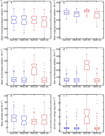
Fig. 7. Distribution of (a) mean incoming longwave radiation,
(b)mean outgoing longwave radiation(c)mean net shortwave
radi-ation,(d)max net shortwave radiation(e)mean sensible flux, and
(f)the resulting 3-day sum of positive energy balance values for
avalanche days (AvD) and non-avalanche days (nAvD) on south-facing (red) and north-south-facing (blue) slopes. Values were calculated with SNOWPACK assuming an elevation of 2500 m and a slope
an-gle of 35◦.
energy is used to melt snow, which helps to narrow down the onset of wet-snow avalanche activity. Some avalanche warn-ing services, e.g. in New Zealand (Conway, 2005), take this fact into account by relating the convergence of snow temper-ature at different heights towards 0◦C to the start of a period with high probability of wet-snow avalanche release. Using simply the daily energy balance allowed detecting 90 % of the wet-snow avalanche days; therefore, energy balance is superior to air temperature in detecting events. However, the problem is that many false alarms resulted, which is not sat-isfying and lowers the overall predictive skill. The true skill score (HK) of the energy balance model was similar to the one of air temperature. Air temperature solely was not suited for predicting the events, but detected non-events fairly well. Combining air temperature with snow surface temperature improved predictive skills (Figs. 4 and 6). For practical ap-plications, these two commonly measured parameters may be well suited, but can only describe flat field conditions.
Fig. 8.Daily maximum amount of liquid water within the
snow-pack for a south-facing 35◦ slope at 2200 m a.s.l. (red solid line)
and 2500 m a.s.l. (blue solid line). Dashed lines show proportion of
snowpack with a zero cold content (red=2200 m; blue=2500 m).
The grey boxes indicate periods with wet-snow avalanche
activ-ity (AAI>2) recorded for the surroundings of Davos, Switzerland,
blue boxes indicate major wet-snow avalanche cycles (AAI>30,
Table 1).
The total amount of liquid water was closely related to days with wet-snow avalanche occurrence on south-facing slopes (Fig. 1), but was generally a poor predictor. Prevailing high amounts of water production and equally a high pro-portion of zero cold content after the major avalanche cy-cle hamper the application of these variables for prediction (Fig. 8). In fact, none of the multivariate approaches used the total amount of water as a variable in its splitting rules. In contrast, the cold content was chosen as splitting rule in the multivariate approaches and seems to be more indica-tive for the onset of wet-snow instabilities. Previous work (Schweizer and Baggi, 2009) supports this fact.
Whether significant melt will affect stability depends not only on the meteorological forcing, but also on snowpack structure (Schneebeli, 2004; Baggi and Schweizer, 2009). Snow stratigraphy at the beginning of the melt season might be quite responsive to the addition of water, while more “ma-ture” or ripe snowpack will not respond to the addition of water. As soon as the snowpack is ripe, an efficient drainage system will be established and water will no longer affect stability (Kattelmann, 1985). In situ measurements captur-ing the above described thermal and mechanical evolution are difficult to perform since changes tend to occur fast, and only represent point observations. Likewise, presently avail-able simulated snow stratigraphy will not depict the com-plex feedback mechanisms of infiltrating water. On the other hand, avalanche activity tended to be widespread and oc-curred within a few days suggesting that the snow cover con-ditions were fairly uniform throughout the area for a certain aspect and elevation. This suggests that forcing by meteoro-logical conditions was overriding local differences in snow stratigraphy and knowing the location and amount of liquid water within the snowpack is not always relevant.
shortwave radiation provides most energy (Fig. 7). As sin-gle parameter it discriminated between event and non-event days for steep (=35◦) southern aspects. Median values on avalanche days were about 80 W m−2, however, maximum values may be as high as 200–400 W m−2 within 60 min (Fig. 7). These maximum flux values might prevail only for 2–4 h per day, but cover around two thirds of the maximum energy input of a single day (Table 4). In case the snow-pack is already at 0◦C, this high energy input during a few hours will be directly transformed into∼1.5 mm of water. On the other hand, the net longwave radiation was in general the largest negative component, i.e. energy loss (Fig. 7). Low negative net values hint to days with cloud cover or a melting snow surface. Cloud cover will attenuate the cooling effect at the snow surface, which will lead to high values forL↑. In fact,L↑was in all statistical models a good splitter (Table 4, Fig. 3).
The values of the turbulent heat fluxes (HSandHL)were
in general lower than half the magnitude of the net irradiative fluxes, but especiallyHS may on some days early in spring
exceed the magnitude of the irradiative terms and therefore needs to be considered when calculating the energy input to the snowpack on a daily basis. It is, however, very diffi-cult to reliably calculateHS for complex terrain. The bulk
method, which is used within SNOWPACK to calculate the turbulent fluxes, provides at best an estimate. It has, how-ever, been shown that the method gives robust results for the location where the data were recorded (Pl¨uss and Mazzoni, 1994). In order to obtain good results for the locations where the input needs to be extrapolated, air temperature, snow sur-face temperature and wind speed have to be representative. None of the three parameters can be verified for the slope simulations. Comparing the air temperature measured at the station Weissfluhjoch (2540 m a.s.l.) to the one at the station Dorfberg suggests that the average lapse rate may be some-what higher than the standard lapse rate of 0.65◦C/100 m. To assess the underestimation we simulatedHSbased on the
data of the station DFB which revealed that the extrapolated value ofHSfor 2200 m was on average 16 % lower. On some
days, however,HS calculated with DFB was 20–30 Wm−2
higher than with the time-lapse approach. Furthermore, the bulk method generally underestimates the sensible heat flux (Arck and Scherer, 2002). Nevertheless, we think that the dif-ference between extrapolation and measurement is accept-able as we compare the meteorological conditions in a given elevation band to the avalanche activity on a regional scale – and not point by point. Our data included only one sig-nificant rain-on-snow event and the above-discussed results on energy balance terms may be biased to situations where irradiation and air temperature caused the melting.
Studying the melt of ice on glaciers is often based on temperature-index models assuming an empirical relation-ship between air temperature and melt rates. Ohmura (2001) has pointed out that air temperature is a reliable proxy for calculating the melt and that considering the full energy
bal-ance does not substantially improve the results. This ap-proach is debatable, but seems to work for glaciological stud-ies (e.g. Braithwaite, 1995). One might therefore conclude that the same approach is applicable for predicting wet-snow avalanches as melt water is closely related to snowpack insta-bility. However, temperature-index models have spatial and temporal deficiencies and rely heavily on the degree-day fac-tor (DDF). The DDF may change with time due to changing albedo and with terrain properties (aspect, slope angle). de Quervain (1979) presented a 28-yr long series of DDF val-ues calculated for the Weissfluhjoch test-site (flat) and con-cluded that a mean value of 4 can be applied for the entire melt period. The DDF values, however, scatter considerably and range from 2.7 to 6.1 depending on whether the melt process was dominated by radiation or air temperature. Ra-diation induced melting was underrepresented by the DDF. Furthermore, our wet-snow avalanches occurred in spring on steep terrain, so that terrain conditions would have to be con-sidered (e.g. Hock, 2003). Whereas temperature-index mod-els provide reasonable results for melt rates when integrated over long time periods, the accuracy decreases with increas-ing temporal resolution, which is a major disadvantage for wet-snow avalanche forecasting. Considering that the 5-day sum of positive air temperature missed most avalanche days (Fig. 5a), indicates that temperature-index models are not suited for our purpose.
Although our analyses are specific to the study area and so are some of the results, such as threshold values, many of the findings can be generalised. For example, for the prediction of the first large melt events, air temperature is not sufficient, but information at least on the thermal state of the snow cover is needed. Calculating energy input and cold content of the snowpack for a specific class of slopes and aspects will pro-vide a good estimate for the first major melt – and hence of potential instability.
7 Conclusions
We compared 4 yr of wet-snow avalanche occurrence in the surroundings of Davos, Switzerland to meteorological data measured by three automated weather stations and to sim-ulated energy balance values. The energy balance was mod-elled for virtual slopes of southern and northern aspects using the 1-D snow cover model SNOWPACK.
Combining various variables in two different multivariate approaches provided satisfactory results. The model based on energy balance variables performed as well as the model using meteorological parameters, but better predicted non-events. Modelling the energy balance for virtual slopes al-lows simulating the energy input, cold content and total amount of water for specific slopes and aspects. The result-ing classification trees clearly demonstrate the importance of the energy input and proportion of cold content for forecast-ing wet-snow avalanches. For both, south-facforecast-ing and north-facing slopes, the energy balance over 3 days was the variable that split best between avalanche and non-avalanche days.
In the presented approach, we focused on external drivers for melt production and did not consider the snowpack stratigraphy and its interaction with melt water. Despite this severe shortcoming, the results are promising for predict-ing wet-snow avalanche activity on a regional scale based on simulated variables using the snow cover model SNOW-PACK. In the future, an approach combining more sophisti-cated water flux models and objective measurement devices, such as upward-looking radar systems, might help to improve prediction accuracy.
Acknowledgements. We would like to thank the editor Michiel van den Broeke, and the reviewers Howard Conway and Karl Birkeland who provided constructive comments that helped to improve the manuscript. C. M. was funded by the Swiss National Science Foundation (SNF, grant 200021-126889). We thank C. Fierz who helped to setup the SNOWPACK simulations and programmed the possibility to deduce the change in cold content within the software. For stimulating discussions we are grateful to F. Techel, B. Reuter, M. Schirmer and M. Lehning. We would like to thank the numerous observers who collected the avalanche occurrence data.
Edited by: M. Van den Broeke
References
Arck, M. and Scherer, D.: Problems in the determination of sensible heat flux over snow, Geogr. Ann. A, 84A, 157–169, 2002. Baggi, S. and Schweizer, J.: Characteristics of wet snow avalanche
activity: 20 years of observations from a high alpine valley (Dis-chma, Switzerland), Nat. Hazards, 50, 97–108, 2009.
Bhutiyani, M. R.: Field investigations on meltwater percolation and its effect on shear strength of wet snow, Proceedings Snow Symp – 94, Manali (H.P.), India, 200–206, 1996.
Braithwaite, R. J.: Positive degree-day factors for ablation on the Greenland ice-sheet studied by energy-balance modeling, J. Glaciol., 41, 153–160, 1995.
Breiman, L.: Random Forest, Mach. Learn., 45, 5–32, 2001. Breiman, L., Friedman, J. H., Olshen, R. A., and Stone, C. J.:
Clas-sification and regression trees, CRC Press, Boca Raton, USA., 368 pp., 1998.
Brun, E. and Rey, C.: Field study on snow mechanical properties with special regard to liquid water content, IAHS-AISH P., 162, 183–193, 1987.
Conway, H.: Storm Lewis: a rain-on-snow event on the Mil-ford Road, New Zealand, Proceedings ISSW 2004, Interna-tional Snow Science Workshop, Jackson Hole WY, USA., 19–24 September 2004, 557–564, 2005.
de Quervain, M.: Schneedeckenablation und Gradtage im Versuchs-feld Weissfluhjoch, Mitteilung Nr. 41 der Versuchsanstalt f¨ur Wasserbau, Hydrologie und Glaziologie an der ETH Z¨urich, 215–232, 1979.
Doswell, A., Davies-Jones, R., and Keller, D.: On summary mea-sures of skill in rare event forecasting based on contingency ta-bles, Weather and Forecast., 5, 576–585, 1990.
Fierz, C. and F¨ohn, P. M. B.: Long-term observation of the wa-ter content of an alpine snowpack, Proceedings Inwa-ternational Snow Science Workshop, Snowbird, Utah, USA, 30 October–3 November 1994, 117–131, 1995.
Hirashima, H., Nishimura, K., Yamaguchi, S., Sato, A., and Lehn-ing, M.: Numerical modeling of liquid water movement through layered snow based on new measurements of the water retention curve, Cold Reg. Sci. Technol., 64, 94–103, 2010.
Hock, R.: Temperature index melt modelling in mountain areas, J. Hydrol., 282, 104–115, 2003.
Kattelmann, R.: Wet slab instability, Proceedings International Snow Science Workshop, Aspen, Colorado, USA, 24–27 Octo-ber 1984, 102–108, 1985.
King, J. C., Pomeroy, J., Gray, D. M., Fierz, C., F¨ohn, P., Harding, R. J., Jordan, R., Martin, E., and Pl¨uss, C.: Snow-atmposphere energy mass balance, in: Snow and Climate, edited by: Arm-strong, R., and Brun, E., Cambridge, 70–124, 2008.
Lehning, M. and Fierz, C.: Assessment of snow transport in avalanche terrain, Cold Reg. Sci. Technol., 51, 240–252, 2008. Lehning, M., Bartelt, P., Brown, R. L., and Fierz, C.: A physical
SNOWPACK model for the Swiss avalanche warning; Part III: meteorological forcing, thin layer formation and evaluation, Cold Reg. Sci. Technol., 35, 169–184, 2002a.
Lehning, M., Bartelt, P., Brown, R. L., Fierz, C., and Satyawali, P. K.: A physical SNOWPACK model for the Swiss avalanche warning; Part II. Snow microstructure, Cold Reg. Sci. Technol., 35, 147–167, 2002b.
Marty, C.: Surface radiation, cloud forcing and greenhous effect in the Alps, Z¨urcher Klima-Schriften, Institut f¨ur Klimaforschung
ETH, Z¨urich, Switzerland, 79, 122,
doi:10.3929/ethz-a-003897100, 2001.
McClung, D. M. and Schaerer, P.: The Avalanche Handbook, 3rd Edn., The Mountaineers Books, Seattle WA, USA, 342 pp., 2006. Mitterer, C., Hirashima, H., and Schweizer, J.: Wet-snow instabili-ties: Comparison of measured and modelled liquid water content and snow stratigraphy, Ann. Glaciol., 52, 201–208, 2011. Ohmura, A.: Physical basis for the temperature-based melt-index
method, J. Appl. Meteorol., 40, 753–761, 2001.
Peitzsch, E. H., Hendrikx, J., Fagre, D. B., and Reardon, B.: Exam-ining spring wet slab and glide avalanche occurrence along the Going-to-the-Sun Road corridor, Glacier National Park, Mon-tana, USA, Cold Reg. Sci. Technol., 78, 73–81, 2012.
Romig, J. M., Custer, S. G., Birkeland, K. W., and Locke, W. W.: March wet avalanche prediction at Bridger Bowl Ski Area, Montana, Proceedings ISSW 2004, International Snow Science Workshop, Jackson Hole WY, USA., 19–24 September 2004, 598–607, 2005.
Schneebeli, M.: Mechanisms in wet snow avalanche release, Pro-ceedings ISSMA-2004, International Symposium on Snow Mon-itoring and Avalanches, Manali, India, 12–16 April 2004, 75–77, 2004.
Schweizer, J., Jamieson, J. B., and Schneebeli, M.:
Snow avalanche formation, Rev. Geophys., 41, 1016,
doi:10.1029/2002RG000123, 2003a.
Schweizer, J., Kronholm, K., and Wiesinger, T.: Verification of re-gional snowpack stability and avalanche danger, Cold Reg. Sci. Technol., 37, 277–288, 2003b.
Schweizer, J., Mitterer, C., and Stoffel, L.: On forecasting large and infrequent snow avalanches. Cold Reg. Sci. Technol., 59, 234– 241, 2009.
Spiegel, M. R. and Stephens, L. J.: Schaum’s outline of theory and problems of statistics, 3rd Edn., Schaum’s outline series, McGraw-Hill, New York, 538 pp., 1999.
St¨ossel, F., Guala, M., Fierz, C., Manes, C., and Lehning, M.: Micrometeorological and morphological observations of surface hoar dynamics on a mountain snow cover, Water Resour. Res., 46, W04511, doi:10.1029/2009WR008198, 2010.
Techel, F. and Pielmeier, C.: Wet snow diurnal evolution and sta-bility assessment, Proceedings ISSW 2009, International Snow Science Workshop, Davos, Switzerland, 27 September–2 Octo-ber 2009, 256–261, 2009.
Techel, F. and Pielmeier, C.: Snowpack properties of unstable wet snow slopes: observations from the Swiss Alps, Proceedings ISSW 2010, International Snow Science Workshop, Lake Tahoe, California, USA, 17–22 October 2010, 187–193, 2010. Techel, F. and Pielmeier, C.: Point observations of liquid water
con-tent in wet snow – investigating methodical, spatial and tempo-ral aspects, The Cryosphere, 5, 405–418, doi:10.5194/tc-5-405-2011, 2011.
Trautman, S.: Investigations into wet snow, The Avalanche Review, 26, 16–17, 2008.
Wilks, D. S.: Statistical methods in the atmospheric sciences: an introduction, International Geophysics, Academic Press, San Diego CA, USA, 467 pp., 1995.
Yamanoi, K. and Endo, Y.: Dependence of shear strength of snow cover on density and water content, Seppyo J. Jpn. Soc. Snow Ice, 64, 443–451, 2002.