Speed Estimation Method for AC Drives

(1)

ELECTROTECHNICS, ELECTRONICS, AUTOMATIC CONTROL, INFORMATICS

SPEED ESTIMATION METHOD FOR AC DRIVES

Marian GAICEANU

Dunarea de Jos University of Galati Domneasca 47, 800008-Galati, Romania

Email: Marian.Gaiceanu@ugal.ro

Abstract: Two structures of speed estimator for AC drive system are developed in this paper. The mathematical models and the simulation results, via numerical simulation, are presented. The utility of the estimator is important for the speed control or for the advanced control synthesis such as optimal vector control of induction motor drives. Besides of speed estimation objective, the proposed method increases the robustness of estimators to measurement signal noises.

Keywords: speed estimation, first order estimator, second order estimator, rotor field oriented control, mathematical model, AC drives.

1.INTRODUCTION

The modern control of AC drives requires more and more information about system states and perturbations. The most important perturbation of a drive is the load torque. The load torque can be measured by using adequate equipment (torque sensor) or can be estimated from a torque estimator. The problem of speed estimation appears at the electric drives with the different speed operation than the synchronous one (Holtz, 1996). Compared to measuring speed, the estimation speed brings some important advantages such as increased reliability and reducing cost. For advanced electric drives (vector control) accurate speed estimation is necessary for a wider speed range of operation than the scalar controlled PWM inverter drives. Various speed estimation methods have been developed for sensorless control of induction motor drives (Mostafa, et al., 2009; Jezernik, et al., 2003; Hossein, 2009; Haron and Idris, 2006; Kim et al, 1994; Proca, and Keyhani, 2007). There are two basic strategies for speed estimation: the first is to use the mathematical model (Holtz,1996; Jezernik, et al.,

2003; Bose, et al., 1995) and the second relies on saliency within induction machine (based on the space harmonics) (Xepapas, et al., 2003; Goran, et al., 2009; Jansen and Lorenz, 1995). The former method depends on the model accuracy having low performances at low rotor frequencies. The later method had obtained very good performance at low speeds. In order to implement this method a complicated hardware is needed for measuring and filtering the stator currents. In order to estimate the speed advanced control techniques were taken into account: model reference adaptive systems (Hossein, 2009; Haron and Idris, 2006; Kalman filtering methods (Kim, et al., 1994); sliding mode (Proca, and Keyhani, 2007; Mezouar, et al., 2008; Goran, et al., 2009) or artificial intelligent methods (Abbou, and Mahmoudi, 2009). Speed estimation plays a key role in sensorless drive. This paper presents simple speed estimation method for vector control drive in rotor field coordinates. For constant flux operation of the induction motor the active stator current is proportional with rotor frequency. Therefore, the torque component of the stator current, isq, can be

(2)

FASCICLE III, 2009, Vol.32, No.2, ISSN 1221-454X magnitude of the stator currents depends on the load

conditions. Hence, the second input of the speed estimator is the applied load torque. The direct measurement of the angular speed is possible by using a speed sensor of from an encoder. By using an encoder, the accurate position can be obtained but expensive equipment is necessary. The second possibility consists of the integration of the mathematical model (Rosu, and Gaiceanu, 1998). Mathematical models of AC drives of higher order were developed including the nonlinearities. Some authors have been used different linearization methods in order to use these models for speed estimation (Barada, et al, 2002). The major disadvantage is that the models integration needs a strong hardware as a digital signal processor.

The proposed method is based on the mathematical model of the induction motor in rotor field coordinates. By using an adequate control (isd=ct),

the nonlinear model becomes linear one which is more adequate for speed estimation purposes. Estimators of 1st and 2nd order are used, which can be implemented easier, because they do not need so complex calculus. The proposed method is distinguished from the others by performance and simplicity. Compared to other estimation methods (Mostafa, et al., 2009; Barada, et al, 2002) the proposed estimators assure high accuracy of the estimated speed over a large range, in stationary and dynamic regimes, especially for low rotor frequency operation.

2.THE MODEL OF THE DRIVE SYSTEM The well-known model of the AC drive using an induction machine in rotor field coordinates supplied

from the current inverter (Fig. 1), is of the form (Murphy, et al., 1998), (Rosu, et al., 1998):

(1)

+

=

+

=

+

mR R

sq m

S e m

sq mR R e

sd mR mR R

i

dt

dq

m

dt

d

J

i

M

p

m

i

dt

di

1

3

2

where:

isd the flux component current; isq the torque component current; imR the rotor magnetizing current;

m the instantaneous angular velocity of the motor; me the electromagnetic torque;

ms the load torque;

J the combined inertia of the motor and load; M the mutual inductance between the stator and the rotor d, q equivalent windings;

R the rotor time constant;

R the rotor leakage factor; p the number of the pole pairs; q the rotor field angle.

There are two different regions for the control of the angular speed: the constant flux and the variable one. In the first case, the constant flux, isd, the flux current component, has a constant value corresponding to the rating flux. This means that the magnetizing current imR has also a constant value and the system (1) gets the form:

(2)

=

+

=

S sq m m

sq q m

m

i

k

dt

d

J

i

k

dt

dq

where

(3) _mR

R

m

i

M

p

k

+

=

1

3

2

and

(4)

mR R q

i

k

=

1

The block diagram of the model (2) is presented in (fig.2) where:

(5)

=

sC sB sA

s s

i

2

3

2

3

0

2

1

2

1

and

(6)

=

s s

sq sd

i

t

q

t

q

t

q

t

q

i

)

(

cos

)

(

sin

)

(

sin

)

(

cos

Obviously, provided by adequate control of the current inverter, the condition isd=ct can be accomplished.

Fig.1.Three-phase squirrel cage induction motor supplied from the c rrent in erter

isA isB

isC 3/2 e -jq is is

isq

isd kq

km -ms

+m

+m q

1/J

Fig.2.The model of the induction machine

M 3 ~

LF

Id

i1A

i1B

i1C 3 ~

(3)

3.THE SPEED ESTIMATOR OF THE SECOND ORDER

The block diagram of the second degree estimator is presented in (Fig. 3), where the input needs the measure of the load torque Ms(s) and the calculus of the torque current component, isq., from the measured stator current. The output of the estimator is the estimated angular speed

ˆ

( )

s

. Therefore, having the transversal current component of the stator current and load torque signals from the adequate transducers the angular speed can be estimated properly. The parameters of the estimator to be determined are c and.

The estimator (Fig. 3), after some manipulations, gets the form presented in (Fig. 4).

Using Laplace transform the second equation from (2) gets the form

(7)

sJ

_m

(

s

)

=

M

(

s

)

M

_s

(

s

)

or in another form

(8)

(

)

1 [

M

(

s

)

M

(

s

)

]

sJ

s

_s

m

=

The closed loop transfer function, H01(s), shown in

the dashed rectangle from Fig. 3, after some manipulations become:

(9)

c

sJ

c

s

H

+

=

)

(

01

This means that the block diagram from (Fig. 3) can be redrawing as in (Fig. 4).

The output of the second order angular speed estimator is obtained from:

(10)

ˆ

(

)

1

[

M

(

s

)

M

ˆ

(

s

)

]

sJ

s

=

_s

or from

(11)

1

1 )

(

)

(

2 ^

+

=

s

c

J

s

_m .

4.CALCULUS OF THE PARAMETERS The problem consists of the calculation of the parameters c and such that the error between the estimated angular speed

ˆ

( )

s

and the actual angular speed m (s) to be insignificant. The transfer function

of the estimator, (Fig.4), is given by: (12)

1

1 )

(

)

(

)

(

2 ^

+

=

s

c

J

s

G

m

Considering a step variation for the m (s), by

setting:

(13)

s

m

=

(

)

the estimated angular speed get the form (14)

)

1 (

1 )

(

2 ^

+

=

s

c

J

s

m

The usual form of the equation (11) is given by (15)

)

1

2 (

1 )

(

0 2 2 0 ^

+

=

s

T

s

T

s

_m

where the damping factor is: (16)

2

0

=

and the pulsation factor (17)

J

c

T

=

2 0 2 0

1

The parameters c and are chosen such as that the response

ˆ

( )

s

to have an acceptable overshoot

(18)

2

1

=

e

,

a small step time response

(19)

2 0

2₎

1 05 . 0 ln(

=

a t

,

and a minimum output noise (Calin S., et al., 1980), (Goodwin, et al., 2001).

Isq(s)

km +

-1/sJ c 1/s

(s) 1/sJ

M(s)

Ms(s)

-H01(s)

Fig.3. Speed estimator of the second order

c

1/s (s) c+sJ

-1/sJ

M(s)

Ms(s)

-Isq(s)

km

m(s)

(4)

FASCICLE III, 2009, Vol.32, No.2, ISSN 1221-454X 5.THE SPEED ESTIMATOR OF THE FIRST

ORDER

The second order estimator has a good behavior regarding to measurement noises, but it implies a relative complex calculus.

The order of the estimator can be reduced as in Fig. 5.

After some manipulations, like for the 2nd degree estimator, the estimator gets the form shown in (Fig.6).

The response to a step input m(s), Fig.7, is given by

(20)

)

1 (

1 )

(

^

+

=

E m s

sT

s

where (21)

c

J

T

_E

=

is the time constant of the estimator. By adequate choosing of the c parameter, respectively time constant TE, an acceptable step response

ˆ

( )

s

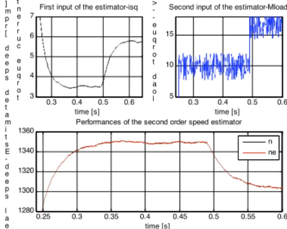
can be obtained.

Fig.7 The input signals (isq and ms), and the comparative results of the real speed (n) with the estimated one (ne) of the second order speed estimator.

Using Z-transform and zero order hold the estimated speed can be calculated. The 1st degree estimator is simpler, but the filtering of the noise is not so good.

0.3 0.4 0.5 0.6 3 4 5 6 7 time [s] First input of the estimator-isq

t o r q u e c u r r e n t

0.3 0.4 0.5 0.6 5

10 15

time [s] Second input of the estimator-Mload

l o a d t o r q u e ->

0.25 0.3 0.35 0.4 0.45 0.5 0.55 0.6 1280 1300 1320 1340 1360 time [s]

Performances of the second order speed estimator

R e a l s p e e d -E s t i m a t e d s p e e d [ r p m ] n ne

Fig.8 More details of the inputs (isq and ms), and the output of the second order speed estimator.

0.25 0.26 0.27 0.28 0.29 0.3 0.31 0.32 0.33 0.34 0.35 1250

1300 1350

time [s]

R e a l s p e e d -E s t i m a

0.49 0.495 0.5 0.505 0.51 0.515 0.52 1300

1320 1340 1360

time [s]

R e a l s p e e d -E s t i m a t e d s p e e d [ r p m ] n ne n ne

Fig. 9. The actual speed (n) and the output response (ne) of the 2nd order speed estimator

0 0.2 0.4 0.6 0.8 -5 0 5 10 15 20 time [s] Second input of the estimator-Mload

0 0.2 0.4 0.6 0.8 0 2 4 6 8 10 time [s] First input of the estimator-isq

-0 0.1 0.2 0.3 0.4 0.5 0.6 0.7 0.8 0

500 1000 1500

time [s]

Performances of the first order speed estimator

R e a l s p e e d -E s t i m a t e d s p e e d [ r p m ] n ne

Fig.10 The input signals (isq and ms), and the comparative results of the real speed (n) with the estimated one (ne) of the first order speed estimator

1/sJ c (s) Isq(s) km 1/sJ M(s)

Ms(s)

-Fig.5.The speed estimator of the first order

m(s)

sJ

c (s)

+

-Fig.6.The simplified block diagram

0 0.2 0.4 0.6 0.8 -10

0 10 20

0 0.2 0.4 0.6 0.8 0

5 10

time [s] First input of the estimator-isq

0 0.1 0.2 0.3 0.4 0.5 0.6 0.7 0.8 0

500 1000 1500

time [s]

(5)

0.3 0.4 0.5 0.6 3

4 5 6 7

time [s] First input of the estimator-isq

0.3 0.4 0.5 0.6 5

10 15

0.25 0.3 0.35 0.4 0.45 0.5 0.55 0.6 1280

1300 1320 1340 1360

time [s]

R e a l s p e e d -E s t i m a t e d s p e e d [ r p m ]

n ne

Fig.11 More details of the inputs (isq and ms), and the output of the first order speed estimator.

0.25 0.26 0.27 0.28 0.29 0.3 0.31 0.32 0.33 0.34 0.35 1250

1300 1350

time [s]

R e a l s p e e d -E s t i m a

0.49 0.495 0.5 0.505 0.51 0.515 0.52 1300

1320 1340 1360

time [s]

R e a l s p e e d -E s t i m a t e d s p e e d [ r p m ]

n ne

Fig. 12. The actual speed (n) and the output response (ne) of the 1st order speed estimator

6.SIMULATION RESULTS

The 1st degree and 2nd degree estimators were numerically simulated for an induction motor drive system K100L-4 FRAME, IEC TYPE, 2.2 KW, 1420 RPM, 3PHASE, 4.8AMPS, 14.81 Nm rated load

torque, J=0.1kgms^2, VALIADIS MANUFACTURER.

The numerical simulations were done for a starting with no-load, under normal torque operation (10Nm, load torque being applied at 0.25s) and for overload (18 Nm at 0.49s) conditions for both estimator types: second (Fig.7-9) and first orders (Fig.10-11). It is well-known that the load torque signal is rich in noises (Fig.8). The parameters of the second order estimator were chosen taking into consideration 0.707 damping factor, and 0.1 ms sampling time. In these conditions the following estimator parameter values were resulted: =1,4104 and c=148. Fig. 7 shows the input signals (the active current, isq,

and the load torque, ms) of the second order speed

estimator and the comparative results of the real speed (n) with the estimated one (ne).

A detailed figure of the above mentioned signals are shown in Fig.8. In Fig. 9 the actual speed (n) and the output response (ne) of the 2nd order speed estimator are shown.

The output of the 1st degree estimator and to an angular speed step is shown in Fig. 8. The 34.88 of the c parameter value of the first order estimator has been taken for TE= 0,3ms time constant. The same

simulations with the second order speed estimator were done under the same load torque conditions for the first order speed estimator. In Figs.10-12 the simulation results of the first order speed estimator are presented. The error of speed estimation is obtained from:

(22)

(

)

(

)

(

)

^

k

=

_m

Analyzing the results obtained from both estimator types (Fig.10 and Fig 12) the lower estimation error is obtained for the second degree speed estimator. The 1st degree estimator is simpler, but in the first moments at applying a step load torque (at 0,25s and 0,49s) the speed error estimation is higher than in the second order speed estimator case. The increased robustness to load torque sensor noises is obtained.

7.CONCLUSIONS

The numerical simulation results confirm the realizing of a good estimation of the angular speed, without using additional equipment in all load conditions: no-load, normal operation conditions and overload for both types of the speed estimators: the first or the second order. The speed estimators presented in this paper can reject the load torque signal noises from the load torque sensor, increasing the robustness of the speed estimated signal. Moreover, compared to existing estimation methods (Mostafa, et al., 2009; Barada, et al, 2002), the proposed one is available with high accuracy over a large speed range (including low rotor frequency), in stationary and dynamic regimes. The rotor field oriented control is the spread method used in drive applications with induction motors. The utility of the estimator is important for the speed control or for the advanced control synthesis (Rosu and Gaiceanu, 1998), with high performances such as optimal vector control of induction motor drives (Rosu, et al., 1998).

8.REFERENCES

Abbou A., and H. Mahmoudi (2009). Performance of a Sensorless Speed Control for Induction Motor Using DTFC strategy and Intelligent Techniques, J. Electrical Systems 3-5.6, pp 64-81 Barada K., Mohanty, Nisit K. De and Aurobinda

(6)

FASCICLE III, 2009, Vol.32, No.2, ISSN 1221-454X CONFERENCE, NPSC 2002,

dspace.nitrkl.ac.in:8080/dspace/bitstream/2080/5 75/1/NPSC_2002.pdf

Bose BK, Simoes MG, Crecelius DR, Rajashekara K, and Martin R (1995). Speed sensorless hybrid vector controlled induction motor drive. In: Proc 1995 IEEE-IAS; 1995., p. 137–43.

Calin, S., s.a. (1980). Tehnica reglarii automate, Editura Didactica si Pedagogica, Bucuresti

Dejan D. Relji, Darko B. Ostoji, and Veran V. Vasi_{(2006). Simple Speed Sensorless Control of} Induction Motor Drive, SIXTH INTERNATIONAL SYMPOSIUM NIKOLA TESLA, Belgrade, SASA, Serbia, www.tesla-symp06.org/papers/Tesla-Sympo06_Reljic.pdf Goodwin C. Graham, Stefan F. Graebe and Mario

Salgado, (2001). Control System Design, Prentice Hall

Goran Petrovic, Tomislav Kilic, and Bozo Terzic, (2009). Sensorless speed detection of squirrel-cage induction machines using stator neutral point voltage harmonics, Mechanical Systems and Signal Processing 23, 931– 939

Haron A.R., and N.R.N. Idris (2006). Simulation of MRAS-based speed sensorless estimation of induction motor drives using MATLAB/ SIMULINK, in: Proceedings of International Conference on Power and Energy, Putra Jaya, pp. 411–415.

Holtz Joachim (1996). Method for speed sensorless control) ,published in K. Rajashekara (Editor) - Sensorless Control of AC Motors, IEEE Press Book

Hossein Madadi Kojabadi (2009) Active power and MRAS based rotor resistance identification of an IM drive, Simulation Modelling Practice and Theory 17, pp. 376–389

Jansen P. L. and R. D. Lorenz (1995). Transducerless position and velocity estimation in

induction and salient ac machines, IEEE Trans. Ind. Appl., vol. 31, no. 2, March/April 1995, pp. 240- 247.

Jezernik K, Edelbaher G, and Rodic M (2003). Sensorless control of induction motor based on estimation of an electromotive force. In: Proc 2003 IEEE international electric machines and drives conference; 2003. p. 631–7.

Kim Y.R., S.K. Sul, and M.H. Park (1994). Speed sensorless vector control of IM using extended Kalman filter, IEEE Trans. Indus. Appl. 30 (5) 1225–1233

Mezouar A., M.K. Fellah, and S. Hadjeri (2008) Adaptive sliding-mode-observer for sensorless induction motor drive using two-time-scale approach, Simulation Modelling Practice and Theory 16, 1323–1336

Mostafa I. Marei , Mostafa F. Shaaban, and Ahmed A. El-Sattar, (2009). A speed estimation unit for induction motors based on adaptive linear combiner, Energy Conversion and Management 50, pp 1664–1670

Murphy, J. M.D, and Turnbull, F. G. (1988). Power Electronic Control of A.C. Motors, Pergamon Press

Proca A.B., abd A. Keyhani, (2007). Sliding-mode flux observer with online rotor parameter estimation for induction motors, IEEE Trans. Indus. Electron. 54 (Issue 2), pp.716–723

Rosu, E., and Gaiceanu, M. (1998). A load torque estimation method for AC Drives, NCED, Craiova.

Rosu, E., Gaiceanu, and M., Bivol, I. (1998). Optimal Control Strategy for AC Drives, PECM '98, Prague