Submitted20 March 2016
Accepted 17 June 2016
Published19 July 2016
Corresponding authors
Bryan Raveen Nelson, [email protected] Behara Satyanarayana, [email protected]
Academic editor
María Ángeles Esteban
Additional Information and Declarations can be found on page 25
DOI10.7717/peerj.2232
Copyright
2016 Nelson et al.
Distributed under
Creative Commons CC-BY 4.0
OPEN ACCESS
The final spawning ground of
Tachypleus
gigas
(Müller, 1785) on the east
Peninsular Malaysia is at risk: a call for
action
Bryan Raveen Nelson1,2, Behara Satyanarayana3,4,5, Julia Hwei Zhong Moh1,
Mhd Ikhwanuddin1, Anil Chatterji6and Faizah Shaharom7
1Institute of Tropical Aquaculture (AKUATROP), Universiti Malaysia Terengganu—UMT, Kuala
Terengganu, Terengganu, Malaysia
2Horseshoe Crab Research Group (HCRG), Universiti Malaysia Terengganu—UMT, Kuala Terengganu,
Terengganu, Malaysia
3Mangrove Research Unit (MARU), Universiti Malaysia Terengganu—UMT, Institute of Oceanography and
Environment (INOS), Kuala Terengganu, Malaysia
4Laboratory of Systems Ecology and Resource Management, Université Libre de Bruxelles—ULB, Brussels,
Belgium
5Laboratory of Plant Biology and Nature Management, Vrije Universiteit Brussel—VUB, Brussels, Belgium 6Biological Oceanography Division, National Institute of Oceanography (NIO), Goa, India
7Institute of Kenyir Research (IPK), Universiti Malaysia Terengganu—UMT, Kuala Terengganu, Terengganu,
Malaysia
ABSTRACT
Tanjung Selongor and Pantai Balok (State Pahang) are the only two places known for spawning activity of the Malaysian horseshoe crab -Tachypleus gigas(Müller, 1785) on the east coast of Peninsular Malaysia. While the former beach has been disturbed by several anthropogenic activities that ultimately brought an end to the spawning activity ofT. gigas, the status of the latter remains uncertain. In the present study, the spawning behavior ofT. gigasat Pantai Balok (Sites I-III) was observed over a period of thirty six months, in three phases, between 2009 and 2013. Every year, the crab’s nesting activity was found to be high during Southwest monsoon (May–September) followed by Northeast (November–March) and Inter monsoon (April and October) periods.
In the meantime, the number of femaleT. gigas in 2009–2010 (Phase-1) was higher
(38 crabs) than in 2010–2011 (Phase-2: 7 crabs) and 2012–2013 (Phase-3: 9 crabs) for which both increased overexploitation (for edible and fishmeal preparations) as well as anthropogenic disturbances in the vicinity (sand mining since 2009, land reclamation for wave breaker/parking lot constructions in 2011 and fishing jetty construction in 2013) are responsible. In this context, the physical infrastructure developments have altered the sediment close to nesting sites to be dominated by fine sand (2.5Xϕ ) with
moderately-well sorted (0.6–0.7σ ϕ), very-coarse skewed (−2.4SKϕ), and extremely
leptokurtic (12.6Kϕ) properties. Also, increased concentrations of Cadmium (from
4.2 to 13.6 mg kg−1) and Selenium (from 11.5 to 23.3 mg kg−1) in the sediment, and Sulphide (from 21 to 28µg l−1) in the water were observed. In relation to the monsoonal
changes affecting sheltered beach topography and sediment flux, the spawning crabs have shown a seasonal nest shifting behaviour in-between Sites I-III during 2009–2011. However, in 2012–2013, the crabs were mostly restricted to the areas (i.e., Sites I and II) with high oxygen (5.5–8.0 mg l−1) and moisture depth (6.2–10.2 cm). In view of the
SubjectsAquaculture, Fisheries and Fish Science, Conservation Biology, Marine Biology
Keywords Anthropogenic disturbance, Conservation and management, Living fossil, Monsoonal impact, Nest shifting behaviour, Seasonal nesting
INTRODUCTION
The surviving horseshoe crab species, three Asian—Tachypleus gigas (Müller,
1785), Tachypleus tridentatus (Leach, 1819), Carcinoscorpius rotundicauda (Latreille,
1802), and one American—Limulus polyphemus (Linnaeus, 1758) persist from the
Ordovician period (Rudkin & Young,2009). Its body with armour-like carapace, degener-ated spines (adult), appendages with setae, spine-like telson, etc., shows their prehistoric appearance clearly (Walls, Berskson & Smith,2002;Ruppert, Fox & Barnes,2004;Smith, Millard & Carmichael, 2009). Of the four species, only C. rotundicaudabreeds in the muddy areas near mangroves while the rest spawn along the intertidal beaches of the estuarine coasts (Cartwright-Taylor et al.,2011;Nelson et al.,2015). The selective nesting behaviour of the crabs is usually facilitated by appendage setae (chemoreceptors) which can sense and detect suitable sandy/muddy substratum for their egg incubation and hatching (Botton,2009).
Horseshoe crabs are encountered only when they come ashore to shallow and surf-protected beaches for nesting. A male crab attached to the rear end of a female crab (using their pedipalps) is distinguished as one mating pair or amplex (Brockmann,2003;
Duffy et al.,2006;Brockmann & Smith,2009). In addition, satellite males - single and available close to the amplexed pairs to fertilize their eggs and, solitary females - if they are alone, are also visible on the beaches (Mattei et al.,2010;Nelson et al., 2015). A female crab is capable of laying 200–300 eggs (Chatterji & Abidi, 1993) in varying depths (10–20 cm) below the sand (Botton, Tankersley & Lovel, 2010). However, its spawning activity is largely governed by season and local environmental (sediment and water) conditions (Smith, 2007; Weber & Carter, 2009). Despite the increased scientific attention on the horseshoe crabs globally (Smith, Millard & Carmichael,
2009; Chatterji & Shaharom,2009; Mattei et al., 2010;Cartwright-Taylor et al., 2011;
Srijaya et al.,2014), their population is consistently decreasing over the years due to natural (e.g., coastal erosion) as well as anthropogenic disturbances (e.g., pollution, overexploitation, etc.) (Jackson, Nordstrom & Smith,2005;Ngy et al.,2007;Faurby et al.,
L. polyphemusis recognised as ‘near threatened’ species, while the remaining three Asian horseshoe crabs are under ‘‘data deficient’’ category in the IUCN red list (IUCN,2016).
In Malaysia, all three Asian horseshoe crabs are available. While T. gigas and
C. rotundicaudaare present in the coastal areas of Peninsular Malaysia, the distribution of T. tridentatusis restricted to East Malaysia (i.e., Sabah and Sarawak) (Chatterji et al.,
2008). Although several researchers in P. Malaysia have worked onT. gigas, most of their findings are based on short-term investigations (e.g.,Zaleha et al.,2010;John et al.,2011;
Kamaruzzaman et al.,2011;Tan, Christianus & Satar,2011;John, Jalal & Kamaruzzaman,
2013). The only long-term (2009–2011) study that examined the nesting behaviour of
T. gigas was carried out byNelson et al.(2015) from Tanjung Selongor. In fact, Tanjung
Selongor and Pantai Balok (in State Pahang) are the only two places known forT. gigas
spawning on the east coast of P. Malaysia. According toNelson et al.(2015), the physical infrastructural developments such as jetty and road/bridge constructions at Tanjung Selongor have already brought an end to the spawning activity ofT. gigas. In the case of Pantai Balok,Zaleha et al.(2012),Tan et al.(2012), andJohn et al.(2012) have observed the spawning populations and nesting behaviour ofT. gigas, but for different months in 2009–2010 with no seasonal cross-checking. Therefore, an assessment on the seasonal impact as well as state-of-the-art information on T. gigas is necessary and still to be ascertained from Pantai Balok.
The present study was aimed at investigating the relationship between the nesting activity ofT. gigasand the environmental (water/sediment) conditions noticed at Pantai Balok. In specific, identification of major environmental factors predisposed by lunar and
monsoonal changes that supportT. gigasspawning formed the main forte of this study. In
recent years, several anthropogenic activities such as sand mining (2009 - to present), land reclamation (2011), and construction of a fishing jetty (2013) also appeared to influenceT. gigaspopulation. At the end, a few recommendations were offered for possible conservation
and management ofT. gigasat Pantai Balok.
MATERIALS AND METHODS
Study area
We recall that Pantai Balok, in State Pahang, is one of the two spawning grounds forT.
gigason the east coast of P. Malaysia (Lat: 3◦56′16.58′′-3◦55′39.33′′N; Long: 103◦22′32.74′′
-103◦22′27.12′′E) (Fig. 1A). River Balok and its tributaries opens here into South China
Sea and provide a regular exchange of water (Fig. 1B). The climate of Pantai Balok is influenced by Northeast (NE) (November–March) and Southwest (SW) monsoons (May– September), separated by two Inter-monsoon (IM) periods (April and October). The
weather—with a temperature varying between 20 and 36 ◦C, is generally hot and humid
(WU,2014). The annual (average) rainfall is about 1710.5 mm and occurs mostly during
September-December. The tides with a range of 0.1–3.4 m are mixed in nature (NHC,2013). Pantai Balok is under sustained human intervention over the last few decades. In addition to the sand mining since 2009 (Fig. 1B), both land reclamation for wave breaker and parking lot constructions in 2011 (Fig. 1D), and fishing jetty construction in 2013
beach condition in 2009–2010, (D) wave breaker/parking lot construction in 2011 and, (E) fishing jetty construction in 2013.
(Fig. 1E) have brought considerable changes to the beach topography, sediment and water characteristics (present study). Local people also catch the mating pairs ofT. gigasfor their food and processed feed preparations (to use in chick and fish farms). In order to carry out the present study, the local fishermen’s association at Pantai Balok was consulted and their permission was obtained.
Sampling protocol
The spawning activity ofT. gigaswas observed over a period of thirty six months in three phases between 2009 and 2013. Phase-1 corresponds to the observations made from July 2009 to April 2010 (for both full moon and new moon periods), while Phase-2 from June 2010 to June 2011 (only for full moon due to financial limitations), and Phase-3 from May 2012 to May 2013 (for full moon and new moon periods). Overall, the dataset represents 15 months of observations each for SW and NE monsoons and 6 months of observations for IM periods. Restricted to a gentle slope in-between high and mid tide markings, the spawning activity ofT. gigaswas found only in a portion of 381 m along the beach at Pantai Balok. The places that have shown regular yield of nests were divided into three sampling sites namely, Site-I (3◦56′15.76′′N, 103◦22′33.96′′E), Site-II (3◦56′12.90′′N,
103◦22′36.62′′E) and, Site-III (3◦56′16.30′′N, 103◦22′40.36′′E) (located 105–142 m apart).
were only considered for the present analysis/interpretation (for complete details, see the
Supplemental Information). In order to have a better understanding on the nesting activity of T. gigasvis-à-vis environmental conditions, the pollution indicating factors such as heavy metal (i.e., Lead (Pb), Chromium (Cr), Selenium (Se), Cadmium (Cd), Copper (Cu) and Zinc (Zn)) concentrations in the sediment; nutrient (i.e., Nitrite (NO−
2), Nitrate
(NO−
3) and Phosphate (PO34−)) and Sulphide (S2−) concentrations in the water were also tested (for Phases 2 and 3).
Biological observations
All sampling sites were visited at night/early morning during high tide for spawning crabs estimation and to mark their nesting locations, whereas in daytime during low tide for
nest/eggs counting. The spawning (male/female) crabs ofT. gigaswere counted by sight
if they are available ashore and by catch (using hand) if they are submerged in water and releasing the air bubbles. The places that shown air bubbles were marked with wooden stakes for nest/eggs counting. The number of nests was obtained through removing the sand at the point of crab imprints (using plastic hand shovel). The egg clutches from
each nest were gently removed and washedin situwith seawater (using 2 mm sieve) to
count the number of eggs. After counting, all eggs were placed back into the same pit and covered by sand. However, the data on overexploitation of the crabs by local fishermen were qualitative (learnt from other villagers more than from our observations) and hence used only for the analysis.
Hydrological observations
The data on surface water quality parameters such as temperature (◦C), salinity (h), pH
and dissolved oxygen (DO) (mg l−1) were obtainedin situusing YSI 556 multi-probe
sensors (YSI Inc., Yellow-Springs, OH, USA). In addition, 1,000 ml of water was collected from each site for laboratory analyses. All samples were first filtered through microglass
filter paper (WhatmanR GF/C 47 mm, England) and then kept in the ice-box. While
the filter paper used for each sample was preserved separately in 90% Acetone for Chl-a
estimation (Parsons, Maita & Lalli,1984), the pH of the filtered water was adjusted to 2 by adding hydrochloric acid (HCl) (to arrest microbial activity and stabilize organic carbon) (USEPA,2004;Wilde et al.,2009). The analyses of nutrients and sulphide were carried out
in the laboratory using spectrophotometer kit (HACH DREL 2400, USA) (HACH,2004;
Magarde et al.,2011).
Sedimentological observations
Both soil temperature (using thermometer, sensitivity: ±0.2 ◦C) and pH (DM-13
Takamura Electric Works, Japan) were recordedin situat the time of nest/egg counting.
A transparent PVC tube with 3′′ diameter and 1 m length (marked up to 50 cm) was
pushed into the sediment and, the depth above the anoxic/black sand layer was measured
as moisture depth at each sampling site. In addition,∼500 g of surface sediment was
collected from each site (using hand shovel) for the laboratory analyses. About 100 g of the sediment was oven dried for 3 days (at 45 ◦C) and then separated into different
fractions (using <63 to 4,000µm sieves) using a mechanical sieve shaker (Retsch AS 200
Coupled Plasma Optical Emission Spectrometry (ICP-OES) (Varian Vista-Pro, USA) (Noriki et al.,1980). The total organic carbon (TOC) in the samples was estimated using
a TOC analyser (Shimadzu, TOC-VCPH, Japan) (Schumacher,2002;USEPA,2004). In
addition, the sediment enrichment factor (Leong, Kamaruzzaman & Zaleha,2003) and
the geo-accumulation index (Din,1992) were derived for understanding the impact of
pollution in the vicinity.
Statistical analyses
The statistical variations within biological and environmental parameters (atP<0.05)
were tested through One-Way ANOVA (using OriginProv.9.1 software), for which the data
obtained for each (select) parameter from every month in Phases 1-3 were considered. In this context, the phase-wise information was treated as (1-3) dependent groups and tested against to the samplings (I-III) sites, monsoon (SW, NE and IM) seasons, and lunar (full moon and new moon) periods as independent groups. The Principle Component Analysis (PCA) was also used to identify the percentage (%) variation between environmental
(sediment and water) parameters andT. gigasegg counts (root-transformed data) (using
PRIMERv.6 software) (Clarke & Gorley,2006). To establish the species-environment relationship, a routine called BEST - amalgamating BIO-ENV and BVSTEP procedures,
in PRIMERv.6 was followed (with 999 permutations). In this context, the Spearman’s
rank correlation coefficients (ρvalues) were considered for denoting positive and negative
impact of the environmental variables onT. gigasnesting sites.
RESULTS
Spawning population and nesting
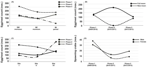
Out of thirty-six months investigation, the spawning activity ofT. gigaswas found only for twenty-two months, especially during SW monsoon followed by NE and IM periods (Tables 1–5) (Fig. 2A). The full moon observations revealed higher egg/nest yield (102–208 nos.) than the new moon observations (82–121 nos.) (Fig. 2B), where the differences were non-significant (Table 6). In total, 117 spawning crabs (males: 63 and females: 54) were recorded for the entire period of investigation. Despite the highest number of spawning crabs at Site-II, Site-III showed maximum egg/nest yield followed by Site-I (Fig. 2C). Although number of the spawning crabs was higher for 2009–2010 (Phase-1: 69 crabs), it
decreased during 2010–2011 (Phase-2: 20 crabs) and 2012–2013 (Phase-3: 28 crabs) (Fig.
2D). Another important observation is that the female crabs dug more number of nests
Figure 2 Egg/nest yield ofTachypleus gigasat Pantai Balok in relation to - (A) season, (B) lunar period, (C) sampling sites and, (D) the number of male and female spawning crabs arriving at Balok beach.
a seasonal nest shifting behaviour from open coastal area (Sites II-III) in SW monsoon to sheltered beach (Site-I) in NE and IM periods (Tables 1–2) (Fig. 6).
Sediment characteristics
The beach sediment that was largely represented by medium sand (1–2Xϕ) in
Phase-1 (Tables 1–2) was changed into fine sand (>2Xϕ ) in Phases 2 and 3 (Tables 3–5).
Categorically, the sediment fraction that contained 0.250 mm (representing medium sand) was more in Phase-1, whereas it replaced by 0.180 mm (representing medium-fine sand) in Phase-2 and 0.125 mm (representing fine sand) in Phase-3. For Phase-1, the sediment was represented by moderately-well sorted to poorly sorted (0.5−1.7σ ϕ), symmetrical to
very-fine skewed (0.0−0.7SKϕ), and very leptokurtic to extremely leptokurtic (2.1−4.6Kϕ)
properties (Tables 1–2). In the case of Phase-2, except skewness (i.e., fine skewed to very-fine skewed: 0.1−3.1SKϕ), both sorting (0.5−1.4σ ϕ) and kurtosis (2.5−20.5Kϕ) remained as
same as Phase-1 (Table 3). The well-sorted to moderately sorted (0.4−1.0σ ϕ), very-coarse
skewed (−3.1− −1.1SKϕ), and extremely leptokurtic (7.8−16.8Kϕ) properties have
characterised the sediment collected for Phase-3 (Tables 4–5). Although there was not much variation in the moisture depth between Phase-1 and Phase-2 (average, 4.2–4.4 cm), it was rather increased in Phase-3 (to 6.8 cm). A significant decrease in (average) silt and
clay, and pH measurements was observed between Phase-1 and Phase-3 (Table 6). The
changes in TOC between Phase-2 and Phase-3 were insignificant, except for SW vs. NE monsoon (Table 6).
In terms of the season, also both fine and medium-fine sand contents (with moderately to moderately-well sorted nature) were high for NE and IM periods whereas more gravel and silt and clay (with poor to moderately sorted nature) for SW monsoon (Tables 1–5). The three sampling sites that represented largely by medium sand (average, 1.4−1.8Xϕ)
and moderate sorting (0.8−1.0σ ϕ) characteristics in Phases 1-2 were replaced by fine
sand (2.5Xϕ) with moderately-well sorted sediment (0.6−0.7σ ϕ) in Phase-3. While
its skewness decreased from symmetrical (0.1SKϕ) to very-coarse skewed (−2.4SKϕ),
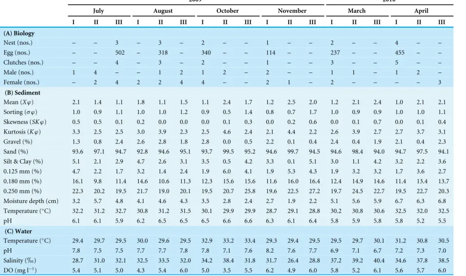
Table 1 Ecobiological observations from the three (I-III) nesting sites ofT achypleus gigasat Pantai Balok during Phase-1 (2009–2010) full moon surveys.
2009 2010
July August October November March April
I II III I II III I II III I II III I II III I II III
(A) Biology
Nest (nos.) – – 3 – 3 – 2 – – 1 – – 2 – – 4 – –
Egg (nos.) – – 502 – 318 – 340 – – 114 – – 237 – – 455 – –
Clutches (nos.) – – 4 – 3 – 2 – – 1 – – 3 – – 5 – –
Male (nos.) 1 4 – – 1 2 1 2 – 2 – – 1 1 – 1 2 –
Female (nos.) – 2 4 2 2 4 4 – – 2 1 – 2 – – – – 3
(B) Sediment
Mean (Xϕ) 2.1 1.4 1.1 1.8 1.1 1.5 1.1 2.4 1.7 1.2 2.5 2.0 1.2 2.1 2.4 1.0 2.1 2.1
Sorting (σ ϕ) 1.0 0.9 1.1 1.0 1.0 1.2 0.9 0.5 1.4 0.8 0.7 1.7 1.0 0.9 0.9 1.0 1.0 1.1
Skewness (SKϕ) 0.5 0.5 0.1 0.2 0.0 0.0 0.0 0.1 0.3 0.0 0.2 0.6 0.0 0.1 0.7 0.0 0.1 0.4
Kurtosis (Kϕ) 3.3 2.5 2.5 3.0 3.9 2.3 2.5 4.6 2.4 2.1 4.4 2.2 2.6 3.9 2.7 2.7 3.7 3.1
Gravel (%) 1.3 0.8 2.4 2.6 2.8 1.8 2.8 0.0 0.5 2.2 0.1 0.4 2.4 0.4 1.9 2.1 0.4 2.3
Sand (%) 93.6 97.1 94.7 92.8 94.6 95.1 93.7 99.5 95.2 94.6 99.7 94.5 94.6 98.4 94.0 94.7 97.5 94.1
Silt & Clay (%) 5.1 2.1 2.9 4.7 2.6 3.1 3.5 0.5 4.2 3.3 0.1 5.1 3.0 1.1 4.2 3.2 2.2 3.6
0.125 mm (%) 4.7 2.2 1.7 3.2 1.4 2.4 1.9 6.0 4.1 1.9 5.3 4.3 1.9 3.2 3.2 1.7 3.6 2.7
0.180 mm (%) 16.1 9.8 11.4 14.6 10.6 11.3 12.3 15.6 15.6 11.6 16.0 16.4 12.4 14.9 14.6 11.4 13.4 13.7 0.250 mm (%) 22.3 20.2 19.5 21.7 19.0 20.1 19.5 20.7 25.8 19.6 22.5 27.2 19.7 24.5 22.7 19.5 22.7 20.3
Moisture depth (cm) 3.2 5.7 4.8 4.1 4.6 4.3 3.5 2.8 2.4 2.7 1.9 2.2 5.1 5.6 5.9 6.7 6.3 6.8
Temperature (◦C) 32.2 31.2 32.7 30.8 31.2 31.5 30.1 29.9 29.9 28.7 29.1 28.8 30.2 30.8 30.6 32.5 32.0 32.5
pH 6.1 6.1 5.9 6.2 6.5 6.5 6.5 6.6 6.6 6.3 6.1 6.4 5.8 5.9 5.8 5.8 5.2 5.5
(C) Water
Temperature (◦C) 29.4 29.7 29.5 30.0 29.6 29.5 32.9 33.2 33.4 29.3 29.4 29.5 29.5 29.7 30.1 31.2 30.8 30.5
pH 7.8 7.5 7.5 7.7 7.7 7.8 7.8 7.1 7.6 8.2 7.6 7.7 6.9 7.1 6.7 7.2 7.3 7.0
Salinity (h) 28.7 31.0 32.1 32.5 33.5 32.0 34.2 38.4 31.8 31.7 26.4 28.8 37.2 39.2 40.4 34.6 37.8 38.5
DO (mg l−1) 5.4 5.1 5.0 4.3 5.4 6.0 5.0 3.5 5.5 6.2 4.9 6.0 5.8 5.2 6.1 5.6 5.7 6.0
Notes.
‘‘–’’ No sample observed at the time of investigation.
(2016),
P
eerJ
,
DOI
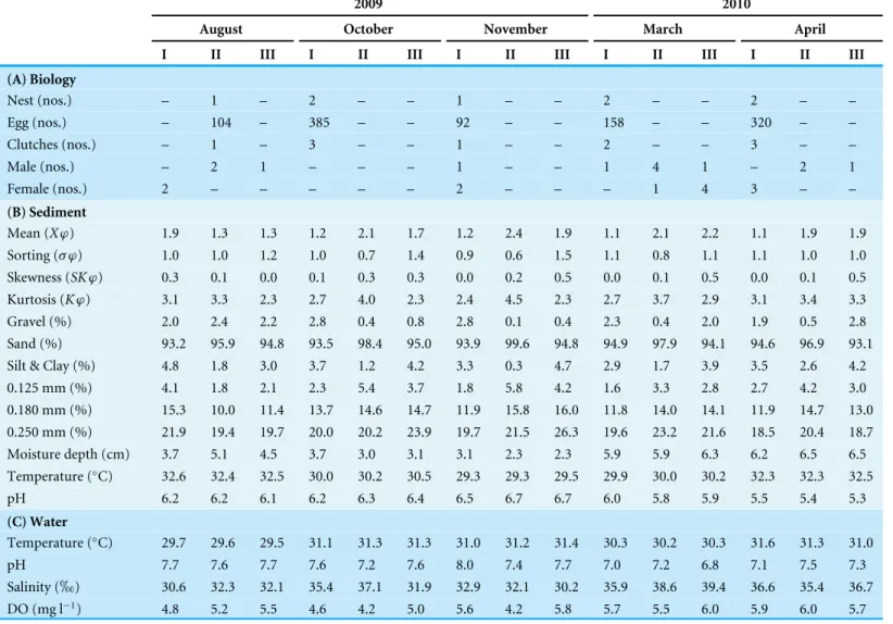
Table 2 Ecobiological observations from the three (I–III) nesting sites ofT achypleus gigasat Pantai Balok during Phase-1 (2009–2010) new moon surveys.
2009 2010
August October November March April
I II III I II III I II III I II III I II III
(A) Biology
Nest (nos.) – 1 – 2 – – 1 – – 2 – – 2 – –
Egg (nos.) – 104 – 385 – – 92 – – 158 – – 320 – –
Clutches (nos.) – 1 – 3 – – 1 – – 2 – – 3 – –
Male (nos.) – 2 1 – – – 1 – – 1 4 1 – 2 1
Female (nos.) 2 – – – – – 2 – – – 1 4 3 – –
(B) Sediment
Mean (Xϕ) 1.9 1.3 1.3 1.2 2.1 1.7 1.2 2.4 1.9 1.1 2.1 2.2 1.1 1.9 1.9
Sorting (σ ϕ) 1.0 1.0 1.2 1.0 0.7 1.4 0.9 0.6 1.5 1.1 0.8 1.1 1.1 1.0 1.0
Skewness (SKϕ) 0.3 0.1 0.0 0.1 0.3 0.3 0.0 0.2 0.5 0.0 0.1 0.5 0.0 0.1 0.5
Kurtosis (Kϕ) 3.1 3.3 2.3 2.7 4.0 2.3 2.4 4.5 2.3 2.7 3.7 2.9 3.1 3.4 3.3
Gravel (%) 2.0 2.4 2.2 2.8 0.4 0.8 2.8 0.1 0.4 2.3 0.4 2.0 1.9 0.5 2.8
Sand (%) 93.2 95.9 94.8 93.5 98.4 95.0 93.9 99.6 94.8 94.9 97.9 94.1 94.6 96.9 93.1
Silt & Clay (%) 4.8 1.8 3.0 3.7 1.2 4.2 3.3 0.3 4.7 2.9 1.7 3.9 3.5 2.6 4.2
0.125 mm (%) 4.1 1.8 2.1 2.3 5.4 3.7 1.8 5.8 4.2 1.6 3.3 2.8 2.7 4.2 3.0
0.180 mm (%) 15.3 10.0 11.4 13.7 14.6 14.7 11.9 15.8 16.0 11.8 14.0 14.1 11.9 14.7 13.0 0.250 mm (%) 21.9 19.4 19.7 20.0 20.2 23.9 19.7 21.5 26.3 19.6 23.2 21.6 18.5 20.4 18.7
Moisture depth (cm) 3.7 5.1 4.5 3.7 3.0 3.1 3.1 2.3 2.3 5.9 5.9 6.3 6.2 6.5 6.5
Temperature (◦C) 32.6 32.4 32.5 30.0 30.2 30.5 29.3 29.3 29.5 29.9 30.0 30.2 32.3 32.3 32.5
pH 6.2 6.2 6.1 6.2 6.3 6.4 6.5 6.7 6.7 6.0 5.8 5.9 5.5 5.4 5.3
(C) Water
Temperature (◦C) 29.7 29.6 29.5 31.1 31.3 31.3 31.0 31.2 31.4 30.3 30.2 30.3 31.6 31.3 31.0
pH 7.7 7.6 7.7 7.6 7.2 7.6 8.0 7.4 7.7 7.0 7.2 6.8 7.1 7.5 7.3
Salinity (h) 30.6 32.3 32.1 35.4 37.1 31.9 32.9 32.1 30.2 35.9 38.6 39.4 36.6 35.4 36.7
DO (mg l−1) 4.8 5.2 5.5 4.6 4.2 5.0 5.6 4.2 5.8 5.7 5.5 6.0 5.9 6.0 5.7
Notes.
‘‘–’’ No sample observed at the time of investigation.
the kurtosis increased from very leptokurtic (2.7Kϕ) to extremely leptokurtic (12.6Kϕ)
between Phase-1 and Phase-3 (Tables 1–5).
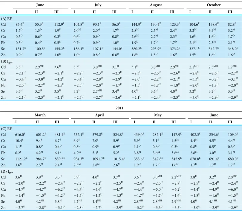
Heavy metal concentrations at the three nesting sites have followed the order of Cr>Zn>Se>Pb>Cu>Cd for Phase-2 (Tables 3–5). In Phase-3, the increased concentrations of Se and Cd at Sites I-II (in the order of Se>Zn>Cr>Cd>Pb>Cu) and increased concentra-tions of Zn, Se, Cd at Site-III (in the order of Zn>Se>Cr>Pb>Cd>Cu) observed. However, in terms of metal induced enrichment at the sampling sites, only Cd and Se have shown their extremity (Tables 7–8). Also, the geo-accumulation index suggests a heavy to extreme con-tamination of both Cd and Se at all sampling sites, especially during 2011–2013 (Tables 7–8).
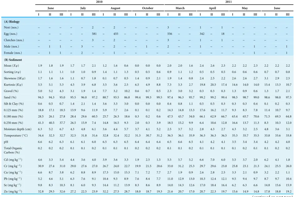
Table 3 Ecobiological observations from the three (I–III) nesting sites ofT achypleus gigasat Pantai Balok during Phase-2 (2010–2011) full moon surveys.
2010 2011
June July August October March April May June
I II III I II III I II III I II III I II III I II III I II III I II III
(A) Biology
Nest (nos.) – – – – – 2 – 2 – – – – 3 – – 1 – 1 – – – – – –
Egg (nos.) – – – – – 581 – 455 – – – – 556 – – 342 – 18 – – – – – –
Clutches (nos.) – – – – – 3 – 2 – – – – 3 – – 1 – 1 – – – – – –
Male (nos.) – 1 1 – 3 – – 2 – – 1 – 2 – – 1 – – – – 1 – – 1
Female (nos.) – 1 1 – 2 – – 1 – – – – – – – – – – – – 1 – – 1
(B) Sediment
Mean (Xϕ) 1.9 1.8 1.9 1.7 1.7 2.1 1.2 1.6 0.6 0.0 0.0 0.0 2.0 2.0 1.6 2.4 2.6 2.3 2.2 2.2 2.3 2.2 2.2 2.2
Sorting (σ ϕ) 1.1 1.1 1.1 1.0 1.0 0.9 1.4 1.1 1.3 0.5 0.5 0.6 0.9 1.1 1.2 0.5 0.5 0.5 0.6 0.6 0.6 0.7 0.7 0.8
Skewness (SKϕ) 1.7 1.6 1.6 1.1 0.7 1.8 0.1 0.7 0.5 1.4 0.9 2.1 1.9 1.4 0.8 2.4 2.5 2.2 2.6 2.6 2.7 3.1 2.9 2.5
Kurtosis (Kϕ) 5.5 5.1 5.3 4.5 3.9 6.8 3.5 3.6 2.5 6.5 4.9 8.8 7.3 5.3 2.7 19.8 20.5 17.4 14.6 14.0 14.0 15.4 13.3 10.7
Gravel (%) 5.0 5.2 4.3 3.1 1.9 1.4 7.7 3.2 10.2 0.6 0.7 0.5 2.3 3.0 3.2 0.3 0.3 0.3 1.3 0.9 0.6 1.3 1.7 2.1 Sand (%) 94.3 94.3 95.0 95.5 96.0 97.2 88.7 93.5 86.8 99.4 99.3 99.5 97.4 96.3 95.7 99.2 99.2 99.4 98.5 98.7 99.0 98.6 98.0 97.5 Silt & Clay (%) 0.6 0.5 0.7 1.4 2.1 1.4 3.6 3.3 3.0 0.0 0.0 0.0 0.4 0.8 1.1 0.5 0.5 0.3 0.3 0.3 0.4 0.1 0.2 0.3 0.125 mm (%) 18.8 17.1 18.5 13.9 9.6 11.9 5.9 7.7 2.6 0.1 0.1 0.2 14.3 14.8 13.3 17.6 16.2 11.7 9.3 8.3 7.8 11.4 10.7 9.7 0.180 mm (%) 28.5 26.1 27.8 28.4 29.6 60.5 25.7 26.3 18.6 0.3 0.2 0.6 47.5 43.7 34.0 66.1 62.9 66.7 63.4 65.7 70.6 71.5 69.3 64.8 0.250 mm (%) 41.3 40.5 37.7 26.5 15.9 7.4 14.8 16.5 9.3 2.0 0.3 3.9 18.5 15.2 9.9 6.4 10.6 12.8 16.6 13.7 11.3 8.3 10.3 12.0 Moisture depth (cm) 6.3 5.2 6.7 4.3 4.8 6.1 3.6 4.4 5.7 3.7 4.1 5.2 2.5 3.7 3.2 2.8 4.3 2.7 4.3 3.2 2.5 4.8 3.6 3.1 Temperature (◦C) 34.4 32.3 32.7 32.5 31.8 31.6 32.8 32.4 32.2 31.3 30.7 31.2 36.5 36.1 35.9 36.3 36.3 36.5 35.3 35.7 35.5 33.8 33.6 33.8
pH 6.6 6.2 6.3 6.1 6.1 6.0 6.5 6.3 6.5 6.4 6.4 6.4 6.5 6.6 6.5 4.1 4.2 4.1 3.5 3.4 3.4 4.2 4.2 4.0 Total Organic
Carbon (%)
0.2 0.2 0.2 0.1 0.1 0.2 0.1 0.1 0.1 0.2 0.2 0.2 0.1 0.1 0.2 0.1 0.1 0.1 0.1 0.2 0.1 0.1 0.2 0.2
Cd (mg kg−1) 4.6 3.3 5.4 4.4 3.6 4.0 3.9 3.6 3.3 1.9 2.5 1.5 5.5 5.7 5.2 6.6 7.0 6.0 5.5 3.7 2.0 6.2 4.1 1.8
Cr (mg kg−1) 30.9 27.4 31.0 29.0 27.6 27.0 26.7 24.0 22.7 19.9 21.5 20.6 33.0 31.2 25.3 29.7 29.6 23.8 25.8 23.1 21.3 24.1 25.5 26.0
Cu (mg kg−1) 6.6 8.7 3.8 6.2 8.8 8.9 17.3 15.0 15.3 7.1 7.2 7.7 2.7 1.9 0.9 2.6 2.8 2.5 3.3 2.1 0.9 3.2 2.2 1.1
Pb (mg kg−1) 5.2 4.6 5.1 6.3 7.6 9.1 10.4 9.3 8.9 7.6 8.4 7.7 11.0 12.9 13.0 10.3 12.4 12.1 9.5 9.4 9.7 8.7 9.7 10.4
Se (mg kg−1) 9.8 8.3 10.3 8.1 6.0 9.3 14.4 11.2 13.9 8.3 8.6 8.9 14.0 14.3 12.6 17.0 18.4 16.4 6.2 6.3 6.6 14.8 15.6 15.9
Zn (mg kg−1) 32.8 29.5 32.6 27.2 22.5 23.9 32.2 27.5 28.7 18.0 18.7 19.3 21.6 20.7 17.0 20.7 22.3 19.7 15.6 14.9 14.8 17.8 18.8 19.2 (continued on next page)
(2016),
P
eerJ
,
DOI
10.7717/peerj.2232
Table 3(continued)
2010 2011
June July August October March April May June
I II III I II III I II III I II III I II III I II III I II III I II III
(C) Water
Temperature (◦C) 29.4 29.5 29.5 29.5 29.6 29.5 30.0 30.0 29.8 29.8 29.6 29.6 30.4 30.2 30.3 29.8 29.9 29.7 30.3 30.4 30.4 30.0 30.1 30.1
pH 7.8 7.5 7.2 7.3 7.6 7.5 7.6 7.8 7.4 7.1 7.5 7.1 6.7 6.2 5.9 6.9 6.5 6.3 8.1 7.7 7.5 8.8 8.4 8.2 Salinity (h) 32.1 32.8 33.6 32.0 32.8 33.6 32.5 32.9 33.3 6.6 10.7 12.0 8.2 9.4 10.2 4.1 5.6 6.4 11.1 12.6 13.3 14.9 15.3 17.0
Dissolved Oxygen (mg l−1)
5.4 5.3 5.3 6.0 5.9 5.8 4.3 4.7 4.8 4.0 3.7 3.4 3.1 3.2 3.4 5.3 5.2 5.2 2.8 3.0 3.1 3.3 3.3 3.3
NO−
2(mg l−1) 0.0 0.0 0.0 0.1 0.1 0.1 0.1 0.1 0.1 0.0 0.0 0.0 0.1 0.1 0.1 0.0 0.0 0.0 0.0 0.0 0.0 0.0 0.0 0.0
NO−
3(mg l−1) 0.9 1.3 1.4 1.4 1.6 1.5 1.1 1.1 0.8 0.3 0.6 0.3 1.5 1.6 1.4 1.1 1.9 1.8 0.8 0.5 0.9 0.6 0.2 0.2
PO3−
4 (mg l−1) 0.3 0.3 0.3 0.3 0.3 0.3 0.4 0.4 0.4 0.3 0.3 0.4 0.4 0.4 0.4 0.1 0.1 0.1 0.4 0.4 0.4 0.4 0.4 0.4
S2−(µg l−1) 1.3 1.7 1.0 4.0 4.7 6.0 11.7 7.0 12.7 15.0 9.0 12.7 31.3 28.7 29.7 68.0 66.0 63.3 14.3 12.7 14.0 27.3 29.0 26.3
Chl-a(mg l−1) 0.1 0.1 0.1 0.1 0.1 0.1 0.0 0.0 0.0 0.1 0.1 0.1 0.1 0.1 0.1 0.0 0.0 0.0 0.1 0.1 0.1 0.1 0.1 0.1
Notes.
‘‘–’’ No sample observed at the time of investigation.
N
elson
e
t
al.
(2016),
P
eerJ
,
DOI
10.7717/peerj.2232
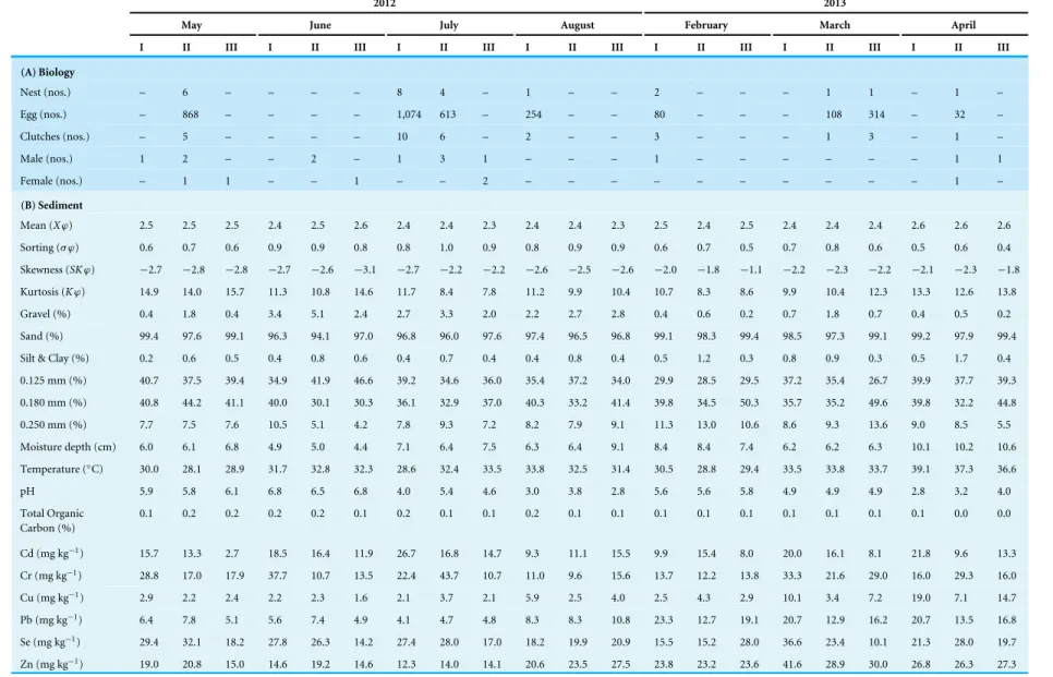
Table 4 Ecobiological observations from the three (I–III) nesting sites ofT achypleus gigasat Pantai Balok during Phase-3 (2012–2013) full moon surveys.
2012 2013
May June July August February March April
I II III I II III I II III I II III I II III I II III I II III
(A) Biology
Nest (nos.) – 6 – – – – 8 4 – 1 – – 2 – – – 1 1 – 1 –
Egg (nos.) – 868 – – – – 1,074 613 – 254 – – 80 – – – 108 314 – 32 –
Clutches (nos.) – 5 – – – – 10 6 – 2 – – 3 – – – 1 3 – 1 –
Male (nos.) 1 2 – – 2 – 1 3 1 – – – 1 – – – – – – 1 1
Female (nos.) – 1 1 – – 1 – – 2 – – – – – – – – – – 1 –
(B) Sediment
Mean (Xϕ) 2.5 2.5 2.5 2.4 2.5 2.6 2.4 2.4 2.3 2.4 2.4 2.3 2.5 2.4 2.5 2.4 2.4 2.4 2.6 2.6 2.6
Sorting (σ ϕ) 0.6 0.7 0.6 0.9 0.9 0.8 0.8 1.0 0.9 0.8 0.9 0.9 0.6 0.7 0.5 0.7 0.8 0.6 0.5 0.6 0.4
Skewness (SKϕ) −2.7 −2.8 −2.8 −2.7 −2.6 −3.1 −2.7 −2.2 −2.2 −2.6 −2.5 −2.6 −2.0 −1.8 −1.1 −2.2 −2.3 −2.2 −2.1 −2.3 −1.8
Kurtosis (Kϕ) 14.9 14.0 15.7 11.3 10.8 14.6 11.7 8.4 7.8 11.2 9.9 10.4 10.7 8.3 8.6 9.9 10.4 12.3 13.3 12.6 13.8
Gravel (%) 0.4 1.8 0.4 3.4 5.1 2.4 2.7 3.3 2.0 2.2 2.7 2.8 0.4 0.6 0.2 0.7 1.8 0.7 0.4 0.5 0.2 Sand (%) 99.4 97.6 99.1 96.3 94.1 97.0 96.8 96.0 97.6 97.4 96.5 96.8 99.1 98.3 99.4 98.5 97.3 99.1 99.2 97.9 99.4 Silt & Clay (%) 0.2 0.6 0.5 0.4 0.8 0.6 0.4 0.7 0.4 0.4 0.8 0.4 0.5 1.2 0.3 0.8 0.9 0.3 0.5 1.7 0.4 0.125 mm (%) 40.7 37.5 39.4 34.9 41.9 46.6 39.2 34.6 36.0 35.4 37.2 34.0 29.9 28.5 29.5 37.2 35.4 26.7 39.9 37.7 39.3 0.180 mm (%) 40.8 44.2 41.1 40.0 30.1 30.3 36.1 32.9 37.0 40.3 33.2 41.4 39.8 34.5 50.3 35.7 35.2 49.6 39.8 32.2 44.8 0.250 mm (%) 7.7 7.5 7.6 10.5 5.1 4.2 7.8 9.3 7.2 8.2 7.9 9.1 11.3 13.0 10.6 8.6 9.3 13.6 9.0 8.5 5.5 Moisture depth (cm) 6.0 6.1 6.8 4.9 5.0 4.4 7.1 6.4 7.5 6.3 6.4 9.1 8.4 8.4 7.4 6.2 6.2 6.3 10.1 10.2 10.6 Temperature (◦C) 30.0 28.1 28.9 31.7 32.8 32.3 28.6 32.4 33.5 33.8 32.5 31.4 30.5 28.8 29.4 33.5 33.8 33.7 39.1 37.3 36.6
pH 5.9 5.8 6.1 6.8 6.5 6.8 4.0 5.4 4.6 3.0 3.8 2.8 5.6 5.6 5.8 4.9 4.9 4.9 2.8 3.2 4.0
Total Organic Carbon (%)
0.1 0.2 0.2 0.2 0.2 0.1 0.2 0.1 0.1 0.2 0.1 0.1 0.1 0.1 0.1 0.1 0.1 0.1 0.1 0.0 0.0
Cd (mg kg−1) 15.7 13.3 2.7 18.5 16.4 11.9 26.7 16.8 14.7 9.3 11.1 15.5 9.9 15.4 8.0 20.0 16.1 8.1 21.8 9.6 13.3
Cr (mg kg−1) 28.8 17.0 17.9 37.7 10.7 13.5 22.4 43.7 10.7 11.0 9.6 15.6 13.7 12.2 13.8 33.3 21.6 29.0 16.0 29.3 16.0
Cu (mg kg−1) 2.9 2.2 2.4 2.2 2.3 1.6 2.1 3.7 2.1 5.9 2.5 4.0 2.5 4.3 2.9 10.1 3.4 7.2 19.0 7.1 14.7
Pb (mg kg−1) 6.4 7.8 5.1 5.6 7.4 4.9 4.1 4.7 4.8 8.3 8.3 10.8 23.3 12.7 19.1 20.7 12.9 16.2 20.7 13.5 16.8
Se (mg kg−1) 29.4 32.1 18.2 27.8 26.3 14.2 27.4 28.0 17.0 18.2 19.9 20.9 15.5 15.2 28.0 36.6 23.4 10.1 21.3 28.0 19.7
Zn (mg kg−1) 19.0 20.8 15.0 14.6 19.2 14.6 12.3 14.0 14.1 20.6 23.5 27.5 23.8 23.2 23.6 41.6 28.9 30.0 26.8 26.3 27.3 (continued on next page)
(2016),
P
eerJ
,
DOI
10.7717/peerj.2232
Table 4(continued)
2012 2013
May June July August February March April
I II III I II III I II III I II III I II III I II III I II III
(C) Water
Temperature (◦C) 27.6 27.6 27.5 29.9 29.6 30.1 30.9 31.3 30.7 30.0 30.1 30.6 28.5 28.7 27.7 30.8 31.1 30.9 32.8 31.6 30.6
pH 6.2 6.5 6.6 8.4 8.4 8.4 8.0 8.1 7.6 7.9 8.4 8.4 7.9 7.7 7.4 8.6 8.7 8.7 8.2 7.9 7.4
Salinity (h) 3.1 2.7 2.3 33.3 33.4 33.3 34.5 34.5 34.6 30.0 31.0 31.2 3.7 3.9 5.4 20.9 21.7 21.7 16.9 15.0 16.7
Dissolved Oxygen (mg l−1)
2.8 3.2 4.1 5.3 5.1 5.6 6.8 5.4 6.7 7.8 5.8 9.1 7.6 5.0 7.9 5.3 6.4 4.5 4.6 6.0 5.5
NO−
2(mg l−1) 0.0 0.0 0.0 0.0 0.0 0.0 0.0 0.0 0.0 0.0 0.0 0.0 0.1 0.1 0.0 0.0 0.1 0.0 0.1 0.1 0.1
NO−
3(mg l−1) 0.2 0.3 0.3 0.7 1.4 0.3 0.7 0.3 0.6 3.4 0.6 0.7 0.4 0.6 0.7 2.9 1.7 2.4 0.6 0.7 0.9
PO3−
4 (mg l−1) 0.1 0.2 0.2 0.0 0.1 0.1 0.1 0.1 0.1 0.0 0.1 0.1 0.2 0.2 0.1 0.2 0.2 0.1 0.2 0.2 0.2
S2−(µg l−1) 47.7 42.3 50.3 20.0 16.3 10.3 5.3 7.3 7.7 39.3 97.3 124.7 23.3 22.0 66.7 0.0 4.7 5.0 58.7 35.7 22.0
Chl-a(mg l−1) 0.2 0.5 0.2 0.4 0.5 0.4 0.4 0.3 0.5 0.7 0.9 0.5 0.6 0.9 0.5 0.4 0.6 0.5 1.0 1.2 1.0
Notes.
‘‘–’’ No sample observed at the time of investigation.
N
elson
e
t
al.
(2016),
P
eerJ
,
DOI
10.7717/peerj.2232
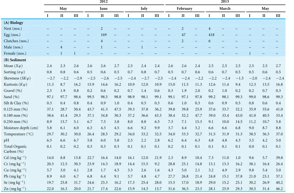
Table 5 Ecobiological observations from the three (I–III) nesting sites ofT achypleus gigasat Pantai Balok during Phase-3 (2012–2013) new moon surveys.
2012 2013
May June July February March May
I II III I II III I II III I II III I II III I II III
(A) Biology
Nest (nos.) – – – – 2 – – – – – 2 – 4 – – – – –
Egg (nos.) – – – – 169 – – – – – 47 – 418 – – – – –
Clutches (nos.) – – – – 4 – – – – – 2 – 6 – – – – –
Male (nos.) – 4 – – 1 – – 1 – – – – – – – – – –
Female (nos.) – 1 1 – – – – – – – – – – – – 1 – –
(B) Sediment
Mean (Xϕ) 2.4 2.3 2.6 2.6 2.6 2.7 2.5 2.4 2.4 2.6 2.6 2.4 2.5 2.5 2.5 2.5 2.5 2.7
Sorting (σ ϕ) 0.8 0.8 0.6 0.5 0.6 0.5 0.7 0.8 0.7 0.5 0.7 0.6 0.6 0.7 0.5 0.5 0.6 0.5
Skewness (SKϕ) −2.7 −2.2 −2.9 −2.5 −2.6 −2.5 −2.4 −2.7 −2.5 −2.4 −2.4 −2.2 −2.2 −2.4 −1.5 −2.0 −2.4 −2.4
Kurtosis (Kϕ) 11.3 8.7 16.2 15.9 14.6 16.2 10.9 12.0 10.9 15.0 11.5 11.3 12.6 11.4 9.4 12.3 13.5 16.8
Gravel (%) 2.5 1.9 0.8 0.2 0.6 0.2 0.7 1.4 0.6 0.3 1.9 2.0 0.2 1.0 0.2 0.2 0.7 0.3
Sand (%) 97.1 97.7 98.4 99.5 98.5 98.8 98.9 98.1 99.1 99.1 97.1 97.8 99.2 98.1 99.3 99.0 98.6 99.3
Silt & Clay (%) 0.3 0.4 0.8 0.4 0.9 1.0 0.4 0.5 0.3 0.6 1.0 0.3 0.6 0.9 0.5 0.8 0.6 0.4
0.125 mm (%) 37.1 28.7 50.4 43.7 41.3 47.5 39.3 37.8 36.2 39.8 39.8 25.9 37.6 33.7 32.2 35.9 35.6 41.0 0.180 mm (%) 38.6 41.4 29.3 37.1 34.8 30.3 37.2 36.6 43.3 38.4 32.2 47.7 39.0 33.4 43.0 41.0 40.5 33.4
0.250 mm (%) 8.9 13.7 5.1 6.7 7.5 3.8 8.0 8.8 6.5 7.3 7.1 15.3 9.1 10.0 14.5 11.2 10.7 5.8
Moisture depth (cm) 5.8 6.1 6.0 6.3 4.3 4.5 6.6 9.2 9.9 3.7 4.4 3.2 6.6 6.6 6.8 9.0 8.7 8.8
Temperature (◦C) 29.7 30.2 30.0 26.4 28.5 29.2 34.0 33.2 32.5 34.0 33.3 32.7 31.5 31.9 31.3 38.5 36.3 37.0
pH 6.5 6.6 6.7 5.8 6.0 5.8 2.5 2.2 2.8 6.2 6.4 6.3 4.8 4.8 4.3 3.5 4.2 5.0
Total Organic Carbon (%)
0.1 0.2 0.2 0.3 0.3 0.3 0.1 0.1 0.1 0.2 0.1 0.1 0.1 0.1 0.1 0.0 0.1 0.1
Cd (mg kg−1) 14.0 8.8 13.8 22.7 16.4 14.0 16.1 12.0 21.9 2.3 8.9 10.4 7.3 11.0 1.0 9.6 5.7 39.8
Cr (mg kg−1) 20.3 12.5 30.3 23.9 14.3 18.9 14.4 15.5 9.2 28.8 25.1 14.8 13.1 13.3 16.2 38.1 16.4 26.4
Cu (mg kg−1) 5.7 3.0 4.1 2.8 1.7 4.5 3.3 2.6 1.6 4.3 5.0 2.1 3.2 4.9 2.9 9.8 5.4 5.0
Pb (mg kg−1) 8.9 6.0 6.7 6.8 6.4 9.1 5.7 4.8 4.7 27.7 26.8 21.4 24.8 15.1 37.8 21.0 23.1 37.1
Se (mg kg−1) 19.7 25.8 31.7 24.6 25.3 16.2 17.3 25.4 28.0 15.5 17.0 18.9 29.0 15.2 25.1 30.2 26.9 40.2
Zn (mg kg−1) 22.0 16.3 20.0 21.7 17.4 22.6 15.9 14.3 13.7 31.6 36.5 23.3 28.1 25.9 29.3 30.5 31.4 46.2
(continued on next page)
(2016),
P
eerJ
,
DOI
10.7717/peerj.2232
Table 5(continued)
2012 2013
May June July February March May
I II III I II III I II III I II III I II III I II III
(C) Water
Temperature (◦C) 29.8 29.7 29.8 29.5 29.7 29.5 29.1 28.9 31.2 30.3 29.6 30.0 29.4 29.6 29.5 30.5 31.4 31.6
pH 6.0 6.2 6.4 8.3 8.3 8.4 7.0 7.5 8.1 8.1 8.1 7.6 8.1 8.1 7.8 8.7 8.6 8.0
Salinity (h) 36.0 35.9 36.8 33.2 33.0 33.1 27.4 28.4 33.5 4.1 4.4 5.4 12.4 12.6 13.9 22.0 23.2 26.2 Dissolved Oxygen
(mg l−1)
7.0 6.8 7.0 6.1 5.5 6.5 5.2 9.1 8.0 7.9 10.8 3.1 6.6 9.6 6.3 6.2 10.0 10.1
NO−
2 (mg l−1) 0.0 0.0 0.0 0.0 0.0 0.0 0.0 0.0 0.0 0.0 0.0 0.0 0.0 0.0 0.0 0.2 0.2 0.1
NO−
3 (mg l−1) 0.5 1.7 1.1 0.3 0.5 0.6 0.7 0.3 0.6 1.4 1.0 0.8 0.9 1.6 1.1 1.9 1.9 0.5
PO3−
4 (mg l−1) 0.3 0.2 0.2 0.4 0.4 0.3 0.1 0.1 0.1 0.2 0.2 0.1 0.3 0.5 0.3 0.3 0.3 0.2
S2−(µg l−1) 2.0 3.0 1.3 41.0 33.3 9.0 5.3 7.3 7.7 48.0 50.3 54.3 25.3 40.3 11.0 13.0 27.3 18.7
Chl-a(mg l−1) 0.2 0.3 0.2 0.5 0.6 0.4 0.5 0.4 0.6 0.6 0.5 0.5 0.4 0.3 0.2 0.5 0.6 0.5
Notes.
‘‘–’’ No sample observed at the time of investigation.
N
elson
e
t
al.
(2016),
P
eerJ
,
DOI
10.7717/peerj.2232
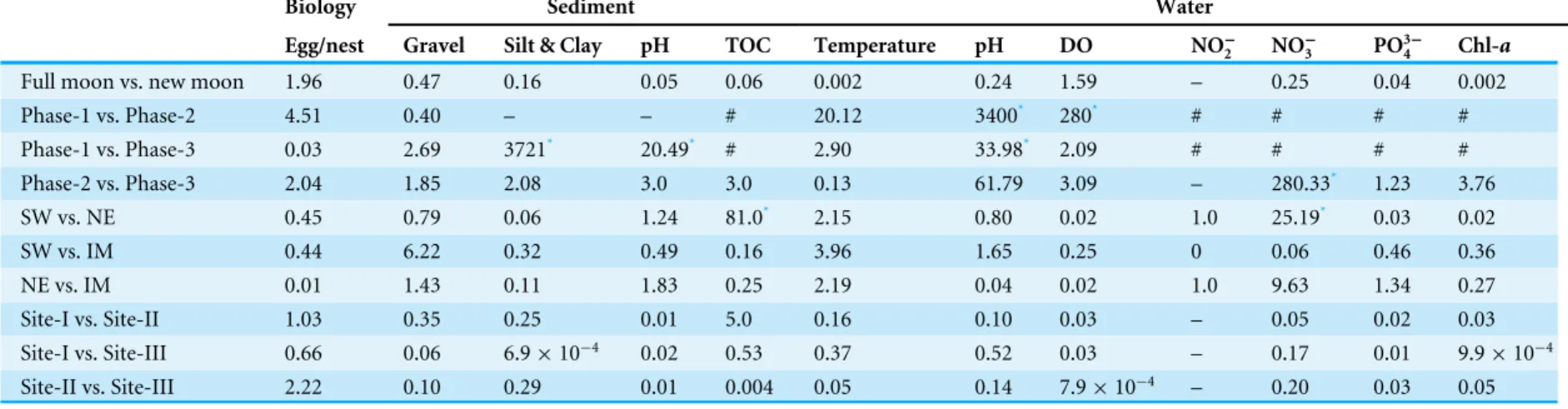
Table 6 Pair-wise statistical variations (Fvalues based on One-Way ANOVA) within biological and environmental parameters in relation to their study phases, sea-sons, sampling sites and lunar periods.
Biology Sediment Water
Egg/nest Gravel Silt & Clay pH TOC Temperature pH DO NO−
2 NO−3 PO34− Chl-a
Full moon vs. new moon 1.96 0.47 0.16 0.05 0.06 0.002 0.24 1.59 – 0.25 0.04 0.002
Phase-1 vs. Phase-2 4.51 0.40 – – # 20.12 3400* 280* # # # #
Phase-1 vs. Phase-3 0.03 2.69 3721* 20.49* # 2.90 33.98* 2.09 # # # #
Phase-2 vs. Phase-3 2.04 1.85 2.08 3.0 3.0 0.13 61.79 3.09 – 280.33* 1.23 3.76
SW vs. NE 0.45 0.79 0.06 1.24 81.0* 2.15 0.80 0.02 1.0 25.19* 0.03 0.02
SW vs. IM 0.44 6.22 0.32 0.49 0.16 3.96 1.65 0.25 0 0.06 0.46 0.36
NE vs. IM 0.01 1.43 0.11 1.83 0.25 2.19 0.04 0.02 1.0 9.63 1.34 0.27
Site-I vs. Site-II 1.03 0.35 0.25 0.01 5.0 0.16 0.10 0.03 – 0.05 0.02 0.03
Site-I vs. Site-III 0.66 0.06 6.9×10⁻⁴ 0.02 0.53 0.37 0.52 0.03 – 0.17 0.01 9.9×10⁻⁴
Site-II vs. Site-III 2.22 0.10 0.29 0.01 0.004 0.05 0.14 7.9×10⁻⁴ – 0.20 0.03 0.05
Notes.
Phase-1: 2009–2010, Phase-2: 2010–2011 and Phase-3: 2012–2013.
SW, Southwest monsoon; NE, Northeast monsoon; IM, Inter-monsoon; TOC, Total Organic Carbon; DO, Dissolved Oxygen; NO−
2, Nitrite; NO−3, Nitrate; PO34−, Phosphate; S2−, Hydrogen
Sul-phide. *P<0.05
‘‘–’’ Data not strong enough for statistical comparison. ‘‘#’’ No Phase-1 observations.
(2016),
P
eerJ
,
DOI
10.7717/peerj.2232
Table 7 Metal induced Enrichment Factor (EF) and Geo-accumulation Index (Igeo) at the three (SI-III) nesting sites ofT achypleus gigasat
Pantai Balok during Phase-2 (2010–2011) survey.
2010
June July August October
I II III I II III I II III I II III
(A) EF
Cd 85.6E 55.3E 112.9E 104.8E 90.1E 86.3E 144.9E 130.4E 123.3E 104.6E 138.6E 82.8E
Cr 1.7D 1.3D 1.9D 2.0M 2.0M 1.7D 2.8M 2.5M 2.4M 3.2M 3.4M 3.2M
Cu 0.5D 0.6D 0.3D 0.6D 0.9D 0.8D 2.6M 2.2M 2.3M 1.6D 1.6D 1.7D
Pb 0.5D 0.4D 0.5D 0.7D 0.9D 1.0D 1.9D 1.7D 1.7D 2.1M 2.3M 2.1M
Se 131.7E 100.5E 155.2E 136.1E 107.1E 144.0E 380.2E 293.9E 373.2E 327.1E 342.7E 348.0E
Zn 0.9D 0.7D 1.0D 1.0D 0.8D 0.8D 1.8D 1.5D 1.6D 1.5D 1.6D 1.6D
(B) Igeo
Cd 3.3H 2.9MH 3.6H 3.3H 3.0MH 3.1H 3.1H 3.0MH 2.9MH 2.1MH 2.5MH 1.7MC
Cr −2.1U −2.3U −2.1U −2.2U −2.3U −2.3U −2.3U −2.5U −2.6U −2.8U −2.6U −2.7U
Cu −3.4U −3.0U −4.2U −3.4U −2.9U −2.9U −2.0U −2.2U −2.1U −3.3U −3.2U −3.1U
Pb −2.5U −2.7U −2.5U −2.3U −2.0U −1.7U −1.5U −1.7U −1.8U −2.0U −1.8U −2.0U
Se 3.5H 3.2H 3.5H 3.2H 2.7MH 3.4H 4.0H 3.6H 4.0H 3.2H 3.2H 3.3H
Zn −2.1U −2.3U −2.1U −2.4U −2.7U −2.6U −2.1U −2.4U −2.3U −3.0U −2.9U −2.9U
2011
March April May June
I II III I II III I II III I II III
(C) EF
Cd 616.0E 601.2E 481.4E 537.1E 579.8E 524.8E 439.0E 282.4E 147.9E 402.3E 254.6E 109.0E
Cr 10.4S 9.4S 6.7S 6.9S 7.0S 5.9S 5.9S 5.1S 4.5M 4.4M 4.5M 4.4M
Cu 1.1D 0.8D 0.4D 0.8D 0.9D 0.9D 1.1D 0.6D 0.3D 0.8D 0.5D 0.3D
Pb 6.2S 4.2M 6.1S 4.2M 5.1S 5.2S 3.8M 3.6M 3.6M 2.8M 3.0M 3.1M
Se 1121.2E 984.7E 839.5E 984.3E 1091.7E 1015.4E 353.6E 342.8E 345.9E 678.8E 691.4E 680.0E
Zn 3.6M 2.5M 2.4M 2.5M 2.8M 2.6M 1.9D 1.7D 1.6D 1.7D 1.7D 1.7D
(D) Igeo
Cd 3.6H 3.9H 3.5H 3.9H 4.0H 3.7H 3.6H 3.0MH 2.2MH 3.8H 3.2H 2.0MC
Cr −2.0U −2.2U −2.4U −2.2U −2.2U −2.5U −2.4U −2.5U −2.7U −2.5U −2.4U −2.4U
Cu −4.7U −4.7U −6.2U −4.7U −4.6U −4.7U −4.4U −5.0U −6.2U −4.4U −4.9U −6.0U
Pb −1.4U −1.5U −1.2U −1.5U −1.3U −1.3U −1.7U −1.7U −1.6U −1.8U −1.6U −1.5U
Se 4.0H 4.2HE 3.8H 4.2HE 4.4HE 4.2HE 2.8MH 2.8MH 2.9MH 4.0H 4.1HE 4.1HE
Zn −2.7U −2.8U −3.1U −2.8U −2.7U −2.9U −3.2U −3.3U −3.3U −3.0U −2.9U −2.9U
Notes.
Cd, Cadmium; Cr, Chromium; Cu, Copper; Pb, Lead; Se, Selenium; Zn, Zinc.
The superscript letters in the Enrichment Factor shows—D, deficiency to minimal enrichment; M, moderate enrichment; S, significant enrichment; E, extremely high enrich-ment. The superscript letters in Geo-accumulation Index shows—U, uncontaminated; MC, moderately contaminated; MH, moderate to heavy contamination; H, heavy con-tamination; HE, heavy to extreme contamination.
Phase-3 (2012–2013) survey.
2012 2013
May June July August Feb March April May
I II III I II III I II III I II III I II III I II III I II III I II III
(A) EF for full moon observations
Cd 296.5E 199.4E 81.6E 523.6E 364.4E 339.5E 737.3E 408.9E 416.6E 213.3E 216.2E 292.4E 193.0E 269.6E 168.6E 215.0E 231.5E 149.7E 372.1E 156.0E 258.2E – – –
Cr 1.5D 0.7D 1.5D 3.0M 0.7D 1.1D 1.8D 3.1M 0.9D 0.7D 0.5D 0.8D 0.8D 0.6D 0.8D 0.9D 0.9D 1.3D 0.8D 1.3D 0.9D – – –
Cu 0.2D 0.1D 0.3D 0.2D 0.2D 0.2D 0.2D 0.4D 0.2D 0.5D 0.2D 0.3D 0.2D 0.3D 0.2D 0.4D 0.2D 0.4D 1.3D 0.4D 1.2D – – –
Pb 0.6D 0.6D 0.8D 0.8D 0.8D 0.7D 0.6D 0.6D 0.7D 0.9D 0.8D 1.0D 2.3M 1.1D 2.0M 1.0D 0.9D 1.3D 1.7D 1.1D 1.7D – – –
Se 396.9E 345.7E 390.0E 555.9E 418.0E 290.9E 547.2E 490.1E 343.3E 292.1E 280.8E 287.9E 216.9E 190.4E 419.8E 287.8E 239.9E 121.6E 253.5E 311.5E 279.1E – – –
Zn 5.3S 4.7S 6.6S 6.2S 6.4S 6.3S 6.4S 5.5S 5.9S 7.0S 6.9S 7.8S 7.0S 6.0S 7.4S 6.1S 6.2S 7.0S 6.6S 6.2S 8.0S – – –
(B) EF for new moon observations
Cd 266.3E 210.4E 290.6E 544.4E 359.6E 317.7E 432.4E 309.2E 634.1E – – – 30.9V 88.6E 218.7E 110.1E 174.6E 19.5S – – – 114.9E 57.9E 572.1E
Cr 1.1D 0.9D 1.8D 1.6D 0.9D 1.2D 1.1D 1.1D 0.8D – – – 1.1D 0.7D 0.9D 0.5D 0.6D 0.9D – – – 1.3D 0.5D 1.1D
Cu 0.4D 0.3D 0.3D 0.3D 0.1D 0.4D 0.4D 0.3D 0.2D – – – 0.2D 0.2D 0.2D 0.2D 0.3D 0.2D – – – 0.5D 0.2D 0.3D
Pb 0.8D 0.7D 0.7D 0.8D 0.7D 1.0D 0.8D 0.6D 0.7D – – – 1.8D 1.3D 2.3M 1.8D 1.2D 3.5D – – – 1.3D 1.1D 2.6M
Se 263.2E 437.4E 457.6E 414.6E 396.7E 262.4E 332.7E 464.6E 574.9E – – – 149.4E 125.4E 283.0E 300.2E 177.1E 351.8E – – – 263.5E 182.6E 408.1E
Zn 6.2S 6.0S 6.1S 7.7S 5.6S 7.6S 6.4S 5.5S 5.9S – – – 6.2S 5.3S 7.4S 6.1S 6.2S 8.2S – – – 5.6S 4.5S 9.7S
(C) Igeofor full moon observations
Cd 5.0HE 4.8HE 2.2MH 5.3EC 5.0HE 4.6HE 5.9EC 5.2EC 5.0EC 4.3HE 4.5HE 5.1EC 4.3HE 4.6HE 4.0HE 5.5EC 5.1EC 3.9H 5.3EC 4.4HE 4.8HE – – –
Cr −2.2U −3.0U −2.9U −1.8U −3.7U −3.3U −2.6U −1.6U −3.7U −3.6U −3.8U −3.1U −3.3U −3.5U −3.3U −2.1U −2.7U −2.3U −3.1U −2.2U −3.1U – – –
Cu −4.6U −4.9U −4.9U −5.0U −4.9U −5.4U −5.1U −4.4U −5.0U −3.5U −4.8U −4.1U −4.8U −4.0U −4.6U −2.8U −4.3U −3.3U −1.8U −3.3U −2.2U – – –
Pb −2.2U −1.9U −2.6U −2.4U −2.0U −2.6U −2.9U −2.7U −2.6U −1.9U −1.9U −1.5U −0.4U −1.2U −0.6U −0.6U −1.2U −0.9U −0.5U −1.2U −0.8U – – –
Se 4.9HE 5.1EC 4.3HE 4.8HE 4.9HE 3.9H 4.9HE 4.9HE 4.2HE 4.3HE 3.5H 4.5HE 4.0HE 4.0HE 4.8HE 5.2EC 4.6HE 3.4H 4.5HE 4.9HE 4.4HE – – –
Zn −2.9U −2.8U −3.3U −3.3U −2.9U −3.3U −3.5U −3.3U −3.3U −2.8U −2.6U −2.4U −2.6U −2.6U −2.6U −1.8U −2.3U −2.3U −2.4U −2.4U −2.4U – – –
(D) Igeofor new moon observations
Cd 4.9HE 4.1HE 4.9HE 5.6EC 5.2EC 4.6HE 5.2EC 4.7HE 5.6EC – – – 2.2MH 4.2HE 4.2HE 3.2H 4.4HE 1.1ME – – – 4.3HE 3.5H 6.3EC
Cr −2.7U −3.4U −2.2U −2.5U −3.2U −2.8U −3.2U −3.1U −3.9U – – – −2.2U −2.5U −3.2U −3.4U −3.3U −3.1U – – – −1.8U −3.1U −2.4U
Cu −3.6U −4.5U −4.0U −4.6U −5.3U −4.1U −4.4U −4.7U −5.4U – – – −4.0U −3.8U −5.1U −4.4U −4.2U −4.6U – – – −2.8U −3.7U −3.8U
Pb −1.8U −2.3U −2.2U −2.1U −2.2U −1.7U −2.4U −2.7U −2.7U – – – −0.1U −0.2U −0.5U −0.3U −1.0U 0.3UM – – – −0.5U −0.4U 0.3UM
Se 4.3HE 4.4HE 5.0HE 4.7HE 4.8HE 4.1HE 4.0H 4.8HE 4.9HE – – – 3.9H 3.9H 4.2HE 5.0HE 3.9H 4.8HE – – – 5.0HE 4.9HE 5.4EC
Zn −2.7U −3.1U −2.8U −2.7U −3.0U −2.7U −3.2U −3.3U −3.4U – – – −2.2U −2.0U −2.6U −2.3U −2.5U −2.3U – – – −2.2U −2.2U −1.6U Notes.
Cd, Cadmium; Cr, Chromium; Cu, Copper; Pb, Lead; Se, Selenium; Zn, Zinc. ‘‘–’’ no sample observed at the time of investigation.
The superscript letters in the Enrichment Factor shows—D, deficiency to minimal enrichment; M, moderate enrichment; S, significant enrichment; V, very high enrichment; E, extremely high enrich-ment. The superscript letters in Geo-accumulation Index shows—U, uncontaminated; UM, uncontaminated to moderately contaminated; ME, moderate contaminated; MH, moderate to heavy
contami-(2016),
P
eerJ
,
DOI
10.7717/peerj.2232
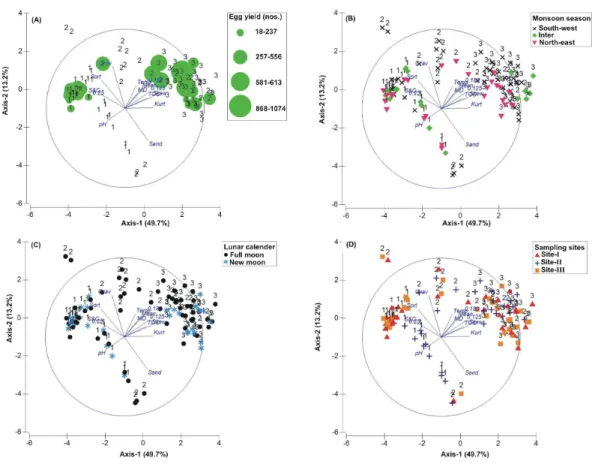
Figure 3 Principal Component Analysis (PCA) showing the % variance in sedimentological param-eters in relation to –(A) Tachypleus gigas egg count, (B) season, (C) lunar period and, (D) sampling sites.The numbers 1–3 indicate study phases in the present investigation (1, 1: 2009-2010; 2, Phase-2: 2010-2011 and 3, Phase-3: 2012-2013). The circle in each panel represents correlation circle and the ori-entation of the environmental (sediment) lines approximate their correlation to the ordination axes. Ab-breviated environmental parameters: Temp, Temperature; Sort, Sorting; Skew, Skewness; Kurt, Kurtosis; Grav, Gravel; S&C, Silt and clay; MD, Moisture depth; and TOC, Total organic carbon.
Water characteristics
Although Phase-2 and Phase-3 observations indicated a general trend of higher salinity
during SW monsoon (25.3–28.0h), followed by IM (7.6–16.2h) and NE periods (9.3–
10.8h) (Tables 3–5), Phase-1 reveals a euhaline (>30h) condition for all three seasons
(Tables 1–2). The seasonal differences in surface water temperature, pH and DO were non-significant (Table 6). Also, the nutrients—NO−
2, NO−3 and PO34−, and Chl-a(observed for Phases 2-3) showed non-significant differences in relation to the seasons, except by NO−
3
for SW vs. NE monsoon. The concentration of S2−was however high for IM (38.9±25
µg
l−1) (mean±SD), followed by NE (29.4±20
µg l−1) and SW (20.8±25µg l−1) in the
order. Overall, the variations in water quality parameters with respect to full/new moon periods, sampling sites and seasons were insignificant (Table 6).
Correlation between biological and environmental parameters
The PCA drawn between biological and sediment parameters showed 49.7% variance along axis-1 (eigenvalue: 6.96), and 13.2% variance along axis-2 (eigenvalue: 1.85) (Fig. 3). The