A class of improved heteroskedasticity-consistent covariance matrix estimators

A CLASS OF IMPROVED HETEROSKEDASTICITY–CONSISTENT

COVARIANCE MATRIX ESTIMATORS

FRANCISCO CRIBARI–NETO

Departamento de Estat´ıstica, CCEN, Universidade Federal de Pernambuco, Cidade Universit´aria, Recife/PE, 50740-540, Brazil

NILA M.S. GALV ˜

AO

Departamento de Ciˆencias Exatas e da Terra, Universidade do Estado da Bahia, Estrada das Barreiras, s/n, Narandiba, Cabula, Salvador, BA, 41195-001, Brazil

Abstract

The heteroskedasticity-consistent covariance matrix estimator proposed by White (1980), also known as HC0, is commonly used in practical applications and is implemented into a number of statistical soft-ware. Cribari–Neto, Ferrari & Cordeiro (2000) have developed a bias-adjustment scheme that delivers bias-corrected White estimators. There are several variants of the original White estimator that also commonly used by practitioners. These include the HC1, HC2 and HC3 estimators, which have proven to have superior small-sample behavior relative to White’s estimator. This paper defines a general bias-correction mechamism that can be applied not only to White’s estimator, but to variants of this estimator as well, such as HC1, HC2 and HC3. Numerical evidence on the usefulness of the proposed corrections is also presented. Overall, the results favor the sequence of improved HC2 estimators.

1. Introduction

Linear regression models oftentimes display heteroskedastic error structures, i.e., non-constant error variances. When that happens the usual ordinary least squares es-timator (OLSE) of the linear parameters remains unbiased and consistent, albeit no longer efficient. Since the exact form of the heteroskedasticity is usually unkown, prac-titioners commonly use the OLSE even when heteroskedasticity is suspected. However, the usual estimator of the OLSE covariance matrix, namely _bσ2(X′X)−1, _bσ2 being an estimator of the common error variance and X the matrix of covariates, is no longer unbiased nor consistent when the homoskedasticity assumption is violated. It then be-comes important to develop and use alternative covariance matrix estimators that are consistent even under heteroskedasticity of unknown form. The most commonly used es-timator is that proposed by Halbert White in an influentialEconometrica paper (White, 1980). White’s estimator, also known as HC0, is implemented into a number of statisti-cal and econometric software (e.g., SHAZAM) and has been used in a variety of empirical analyses. A shortcoming of this estimator is that, although consistent, it can be quite biased in samples of typical size. In particular, it tends to underestimate the true vari-ances, thus leading to associated quasi–t tests that are liberal. Cribari–Neto, Ferrari & Cordeiro (2000) have recently obtained a sequence of bias adjusted White estimators. The first corrected estimator in this sequence is obtained by bias-correcting the White estimator, the second adjusted estimator follows from applying a bias-correction to the first adjusted estimator in the sequence, and so on. The further down one advances in the sequence, the smaller the order of the bias of the corresponding estimator.

There are several alternative estimators that have been proposed in the literature, the most cited ones being the HC1, HC2 and HC3 estimators, the latter closely ap-proximating the jackknife estimator. The finite-sample behavior of these estimators are usually superior to that of HC0 since they already incorporate small-sample cor-rections. Numerical evidence favors these estimators over the White estimator. For instance, the results in Cribari–Neto & Zarkos (1999) favor the HC2 estimator while the results reported by Long & Ervin (2000) and MacKinnon & White (1985) favor the HC3 estimator.

2. The model and some covariance matrix estimators

The model of interest if the usual linear regression model, which is defined as y = Xβ+u, wherey and uare n-vectors of responses and random errors, respectively, β is a p-vector of unknown parameters (p < n), andX is an n×p matrix of fixed regressors with full column rank, i.e., rank(X) = p. We make the following assumptions:

i) E(ut) = 0, t= 1, . . . , n;

ii) E(u2_t) =σ_t2, 0< σ_t2 <∞, t= 1, . . . , n; iii) E(utus) = 0 for all t6=s;

iv) limn→∞(X′X/n) = Q, whereQ is a positive definite matrix.

The ordinary least squares estimator of β is βb = (X′X)−1X′y. It has mean β (i.e., it is unbiased) and covariance matrix Ψ =PΩP′, whereP = (X′X)−1X′ and Ω = cov(u) is a diagonal matrix with the tth diagonal element representing the variance σ_t2 of ut, t = 1, . . . , n. For,

Ψ = cov(βb) = cov[β+ (X′X)−1X′u] = cov[(X′X)−1X′u] = (X′X)−1X′cov(u)X(X′X)−1 = (X′X)−1X′ΩX(X′X)−1.

Under homoskedasticity, we have σ_t2 = σ2, a strictly positive finite constant, for all t, and it thus follows that cov(βb) = σ2(X′X)−1, which can be estimated by bσ2(X′X)−1, where bσ2 = bu′bu/(n−p), bu = (bu1, . . . ,bun)′ = M y being the n-vector of OLS residuals. Here, M = I −H, I is the n ×n identity matrix, and H = X(X′_X)−1_X′ _{(the ‘hat}

matrix’) is symmetric and idempotent.

The unbiasedness of βbcan be easily established:

E(βb) = E[β+ (X′X)−1X′u] =β+ (X′X)−1E(u) = β.

This property is true even under heteroskedasticity.

It is also possible to establish the consistency of the OLSE without assuming ho-moskedasticity. Note that βb=β+ (X′_X)−1_X′_{u and}

plim(βb) = plim[β+ (X′X)−1X′u] =β+ plim³X

′_X

n ´−1

plim³X

′_u

n ´

,

where plim denotes limit in probability. Using Slutsky’s theorem (e.g., Rao, 1973, p. 122), we obtain

plim(βb) =β+³limX

′_X

n ´−1

plim³X

′_u

n ´

.

Pn

t=0Xt′E(ut) = 0, it thus follows from Chebyshev’s weak law of large numbers (e.g., Rao, 1973, p. 112) that

plim³X

′_u

n ´

= 0.

Therefore, plim(βb) = β+Q−10 = β. That is, βb is consistent for β. Again, it was not necessary to assume equal error variances to obtain the result.

Sinceβbis unbiased and consistent even under heteroskedasticity of unknown form, it is commonly used by practitioners when heteroskedasticity is suspected. It is necessary, however, to obtain a consistent estimator for its covariance matrix.

White (1980) proposed a covariance matrix estimator which is consistent under both homoskedasticity and heteroskedasticity of unknown form; it is given by

b

Ψ =PΩbP′, (1)

where

b

Ω = diag{bu21, . . . ,bu2n}.

The idea is to obtain a consistent estimator for the symmetric matrixX′_{ΩX (say,X}′_ΩbX)

that, unlike Ω, has at most p(p+ 1)/2 different elements, regardless of the sample size. That is, plim(X′ΩbX/n) = plim(X′ΩX/n),as n→ ∞. Therefore,

b

Ψ = n(X′X)−1(X′ΩbX/n)(X′X)−1 = (X′X)−1X′ΩbX(X′X)−1,

can be used to consistently estimate the covariance matrix ofβb. The proposed estimator uses, as pointed out above, Ω = diagb {_bu2₁, . . . ,_bu2_n}, and is also known as HC0.

White’s estimator is useful since it allows practitioners to perform inference which is asymptotically correct regardless of the presence of heteroskedasticity in the data or even of the form of such heteroskedasticity if it indeed exists. However, this estimator can be substantially biased in small samples: it tends to underestimate the true variances, thus being a bit too optimistic. In order to overcome this shortcoming, other estimators have been proposed and are also widely used. They can also be written as (1), but with different structures for Ω. The HC1 estimator (Hinkley, 1977) usesb

b

Ω = n

n−pdiag{bu 2

1, . . . ,bu2n}.

It thus includes a finite-sample correction, namely n/(n−p), which accounts for the fact that the OLS residuals tend to fluctuate less than the unknown errors. The HC2 estimator uses

b

Ω = diag ½

b u2₁

1−h1, . . . , b u2_n 1−hn

whereh1, . . . , hn are the diagonal elements ofH. These quantities are usually viewed as measures of the leverage of the corresponding observations. The HC3 estimator discounts the squared residuals more heavily; it uses

b

Ω = diag ½

b u2₁

(1−h1)2, . . . , b u2_n (1−hn)2

¾ .

The finite-sample corrections included in the definition of the HC2 and HC3 estimators are therefore based on the degrees of leverage of the different observations. Since 0 < ht < 1 for all t, the greater ht, the more we inflate the tth squared residual. This is because, as noted by Chesher & Jewitt (1987, p. 1219), the possibility of severe downward bias in the White estimator arises when there are large ht, because the associated least squares residuals have small magnitude on average and the White estimator takes small residuals as evidence of small error variances.

The HC2 estimator, initially proposed by Horn, Horn & Duncan (1975), can be shown to be unbiased under homoskedasticity. Note that E(_bu) = E(M y) = E[M(Xβ−

u)]. Since M X = (I−H)X = 0 it follows that E(_bu) = E(M u) = 0, and hence

E(_bu_bu′) = cov(_bu) + E(_bu)E(_bu′) = cov(M u) = MΩM′.

When the model is homoskedastic, we have that Ω = σ2I. Since M is symmetric and idempotent, we obtain

E(_bu_bu′) =M σ2IM =σ2M =σ2(I−H),

where each diagonal element is given by E(_bu2_t) =σ2(1−ht).

The four covariance matrix estimators presented above are commonly used by prac-titioners and have implementations in several econometric and statistical software, such as Shazam (http://www.shazam.econ.ubc.ca), Stata (http://www.stata.com) and gretl(http://gretl.sourceforge.net). The next section develops bias adjusted ver-sions of these estimators. The biases of the corrected estimators are shown to converge faster to zero than those of the unmodified estimators.

3. A class of improved covariance matrix estimators

We consider the four covariance matrix estimators described in the previous section, namely:

b

Ψi = (X′X)−1X′Ωib X(X′X)−1 =PΩib P′, i= 0,1,2,3.

HC0 : D0=I,

HC1 : D1= µ

n n−p

¶ I,

HC2 : D2= diag{1/(1−ht)},

HC3 : D3= diag{1/(1−ht)2},

where again ht is the tth diagonal element of H = X(X′X)−1X′ and I is the n×n identity matrix. This notation will allows us to treat the four estimators in a unified manner.

At the outset, note that Ω can be written asb Ω = (b bubu′)_d, where bu is the vector of OLS residuals and the subscriptd denotes that a diagonal matrix was formed out of the original matrix by setting all non-diagonal elements equal to zero. We then have that

E(bΩ) = E{(_bu_bu′)d}={E(bubu′)}d ={MΩM}d

={(I −H)Ω(I−H)}_d ={HΩ(H−2I) + Ω}d.

Therefore,

E(Ωi) = E(b DiΩ) =b DiE(Ω) =b Di{HΩ(H−2I) + Ω}d ={DiHΩ(H−2I) +DiΩ}d.

The mean of the estimator Ψib is thus given by

E(Ψi) = Eb {PΩib P′}=PE(Ωi)b P′=P{DiHΩ(H−2I) +DiΩ}dP′.

Using the equations above we obtain the bias function of Ωi:b

B_bΩ

i(Ω) = E(

b

Ωi)−Ω = {DiHΩ(H−2I) +DiΩ}d−Ω.

Since the matrix DiΩ is diagonal, for all i, we can write

B_bΩ

i(Ω) ={DiHΩ(H−2I)}d+DiΩ−Ω

=Di{HΩH−2HΩ}d+ (Di−I)Ω (2)

and

B_bΨ

i(Ω) = E(

b

Ψi)−Ψ =PE(Ωi)b P′−PΩP′ =P{B_bΩ

i(Ω)}P ′

=P[Di{HΩH−2HΩ}d+ (Di−I)Ω]P′. (3)

the exact bias of any of the four estimators described in the previous section by using the corresponding expression for the diagonal matrix Di.

The next step is to define sequences of bias adjusted covariance matrix estimators, denoted {Ψb(k)_i , k = 1,2, . . .}, i= 0,1,2,3, for the covariance matrix of βb. At the outset, we define sequences of adjusted estimators for Ω, say {Ωb(k)_i , k = 1,2, . . .}, i = 0,1,2,3, which will be used to deliver sequences of improved estimators for Ψ.

Consider the recursive function M(k+1)(A) = M(1)(M(k)(A)), k = 0,1,2, . . . , with M(1)(A) = {HA(H−2I)}d e M(0)(A) =A, where H is defined as before and A is an n×n diagonal matrix. It is possible to show that the following properties hold. Let A and B be n×n diagonal matrices, and let k = 0,1,2, . . .. Then:

[P1] M(k)(A) +M(k)(B) =M(k)(A+B);

[P2] M(k)({HA(H−2I)}d) =M(k)(M(1)(A)) =M(k+1)(A);

[P3] E{M(k)(A)}=M(k)(E(A)).

Using the notation and properties outlined above, it is possible to write (2) and (3), respectively, as

B_bΩ

i(Ω) =DiM

(1)_{(Ω) + (D}

i−I)M(0)(Ω)

=Di[M(0)(Ω) +M(1)(Ω)]−M(0)(Ω) (4)

and

B_bΨ

i(Ω) =P{Di[M

(0)_{(Ω) +M}(1)_(Ω)]−M(0)_(Ω)}P′_{, (5)}

for i= 0,1,2,3. An estimator for Ω can be defined as

b

Ω(1)_i =Ωib −B_bΩ

i(Ω) =b Ωib − {Di[M

(0)_{(Ω) +b M}(1)_{(Ω)]b −M}(0)_{(Ω)b },}

where the last equality follows from (4). Since Ωbi = DiΩ andb M(0)(Ω) =b Ω, we haveb that

b

Ω(1)_i =DiM(0)(Ω)b −DiM(0)(Ω)b −DiM(1)(Ω) +b M(0)(Ω) =b M(0)(Ω)b −DiM(1)(Ω)b

=Ωb −DiM(1)(Ω)b . (6)

Note that it would not be feasible to compute the bias of Ωi, since it is a function ofb Ω. Replacing Ω by Ω, we obtain the adjusted estimator defined in (6), which is nearlyb unbiased. Any bias in this estimator is due solely to the fact that M(1)(Ω) is used inb place of the unknown matrix M(1)(Ω). The next step is, thus, to correct for any bias induced by the estimation of B_bΩ

The bias of Ωb(1)_i can be written as

B_b

Ω(1)_i (Ω) = E{Ωb −DiM

(1)_{(Ω)b } −Ω}

=B_bΩ(Ω)−DiE{M(1)(Ω)b −M(1)(Ω)} −DiM(1)(Ω).

Note that Ω0b = D0Ω =b Ω, sinceb D0 = I. Thus, using (4) we arrive at B_bΩ(Ω) = B_bΩ

0(Ω) =M

(1)_{(Ω).Finally, using properties [P1] and [P3], it follows that}

B b

Ω(1)_i (Ω) =M

(1)_(Ω)−D

iM(1)(M(1)(Ω))−DiM(1)(Ω)

=M(1)(Ω)−DiM(2)(Ω)−DiM(1)(Ω), that is,

B b

Ω(1)_i (Ω) =M

(1)_(Ω)−D

iM(1)(Ω)−DiM(2)(Ω). (7)

Applying again the procedure described above and results (6) and (7), we define a second corrected estimator for Ω, namely:

b

Ω(2)_i =Ωb(1)_i −B_bΩ(1)

i

(Ω)b

=Ωb −DiM(1)(Ω)b − {M(1)(Ω)b −DiM(1)(Ω)b −DiM(2)(Ω)b }

=Ωb −M(1)(Ω) +b DiM(2)(Ω)b .

The procedure can be repeated recursively, and after k iterations we arrive at

b Ω(k)_i =

k−1 X

j=0

(−1)jM(j)(Ω) + (b −1)kDiM(k)(Ω)b , k = 1,2, . . . , (8)

fori= 0,1,2,3. The bias ofΩb(k)_i can be derived using properties [P1]—[P3] and equation (8) as

B_bΩ(k)

i

(Ω) = E(Ωb(k)_i )−Ω

= En k−1 X

j=0

(−1)jM(j)(Ω) + (b −1)kDiM(k)(Ω)b o

−Ω

= k−1 X

j=0

(−1)jE{M(j)(Ω) + (b −1)kDiM(k)(Ω)b } −Ω

= k−1 X

j=0

(−1)j{E[M(j)(Ω)b −M(j)(Ω)] +M(j)(Ω)}

+ (−1)kDiE[M(k)(Ω)b −M(k)(Ω)] + (−1)kDiM(k)(Ω)−Ω

Therefore, we define sequences {Ωb(k)_i , k = 1,2, . . .}, i = 0,1,2,3, of estimators for Ω with Ωb(k)_i and their biases given in (8) and (9), respectively. We shall now define sequences of estimators for Ψ, say {Ψb(k)_i , k = 1,2, . . .}, i= 0,1,2,3, where

b

Ψ(k)_i =PΩb(k)_i P′, k = 1,2, . . . , (10)

fori= 0, . . . ,3, so thatΨb(k)_i denotes theith estimator, corrected up to thekth iteration. The bias of Ψb(k)_i follows from (9) and (10) as

B_Ψb(k)

i

(Ω) = E(Ψb(k)_i )−Ψ =PE(Ωb(k)_i )P′−PΩP′=P{B_bΩ(k)

i

(Ω)}P′

= (−1)kP{DiM(k+1)(Ω) +DiM(k)(Ω)−M(k)(Ω)}P′. (11)

Equation (11) yields a closed-form expression for the biases of the different estimators for Ψ corrected up to the kth iteration.

We can now obtain the orders of the biases of the sequences of corrected estimators. From assumption (iv) we have that lim (X′X/n) =Q, as n → ∞, where Q is a positive definite matrix. Equivalently, we have that X′X = O(n), and therefore (X′X)−1 = O(n−1). It then follows that:

1. The matrices P = (X′_X)−1_X′ _{and H = X(X}′_X)−1_X′ _{are O(n}−1_{). In particular,} the diagonal elements of H, ht for t= 1, . . . , n, converge to zero as the sample size increases, i.e., ht =o(1), for all t, which means that the regression design must be balanced in large samples.

2. The elements of the matrices Di’s, defined earlier, converge to finite constants as n → ∞, i.e., Di=O(1) for alli.

Using the above results it can be shown that for a given diagonal matrixAsuch that A=O(n−r), for some r≥0, then

1. P AP′=O(n−(r+1));

2. M(k)(A) =O(n−(r+k)) =DiM(k)(A), i= 0,1,2,3.

Also, from assumption (ii) we have that Ω =O(1). It is now easy to obtain the order of the biases of the sequences of estimators in (8) and (10).

As defined in (9), B_bΩ(k)

i

(Ω) = (−1)k{DiM(k+1)(Ω) +DiM(k)(Ω)−M(k)(Ω)}, and thus

B_bΩ(k)

i

(Ω) =O(n−(k+1)).

We also establish that

B_Ψb(k)

i

(Ω) =O(n−(k+2)).

In order to be general, we shall next consider the variance estimation of linear combinations of the elements of βb. Letc denote a p×1 vector of constants so that c′_βb

defines a linear combination of the elements of βb. Note that

φ = var(c′βb) =c′[cov(βb)]c=c′Ψc.

Thus, a sequence of corrected estimators for φ can be defined as

b

φ(k)_i =c′Ψb(k)_i c, i= 0,1,2,3, (12)

withk = 0 corresponding to the original HCs, as functions of the differentDi’s matrices. The quantity c′Ψb(k)_i cthen represents the ith estimator for the variance ofc′βb, corrected up to the kth iteration.

LetVi = diag{vi12, . . . , vin2 }= (vivi′)d be a matrix withvi=Di1/2P′cfor i= 0,1,2,3, and let the matrices Di’s be as defined earlier, such that

b

φi=c′Ψib c=c′PΩib P′c=c′P DiΩbP′c=c′P D1/2i ΩbD 1/2

i P′c=vi′Ωbvi.

Since Ω = (b bubu′)d, it follows that

b

φi=vi′[(bubu′)d]vi =bu′[(vivi′)d]bu=bu′Vibu, i= 0,1,2,3.

Additionally, since Ω = (b bubu′)d, we have that

b

φi=vi′[(bubu′)d]vi =bu′[(vivi′)d]bu=bu′Vibu, i= 0,1,2,3.

Therefore, φbi=c′Ψib ccan be defined as a quadratic form in the OLS residuals. Similarly,

b

φ(1)_i =c′PΩb(1)_i P′c=c′P{Ωb−DiM(1)(Ω)b }P′c=c′PΩbP′c−c′P D_i1/2M(1)(Ω)b D1/2_i P′c

=c′Ψ0b c−v_i′{HΩ(b H−2I)}_dvi =bu′V0bu− n X

s=1 b

αsvis2, (13)

where bαs is the sth diagonal element of the matrix {HΩ(b H−2I)}d and vis is the sth element of the vector vi,i= 0,1,2,3. Since αbs =Pnt=1h2stbu2t −2hssbu2s, where hst is the (s, t) element of the matrixH, the summation in (13) can be computed as follows:

n X

s=1 b αsvis2 =

n X

s=1

v_is2α_bs = n X

s=1 v2_is

µ_Xn

t=1

h2_stbu2_t −2hssbu2s ¶ = n X s=1 n X t=1

v_is2h2_stbu2_t −2 n X

s=1

v_is2hssbu2s = n X

t=1 b u2_t

µ_Xn

s=1

h2_stv_is2 −2htt2it ¶

We thus obtain

b

φ(1)_i =_bu′V0bu− n X

t=1 b

u2_tbδit, (14)

wherebδit =Pn_s=1h2stvis2 −2httvit2 is thetth diagonal element of {HVi(H−2I)}d. Equa-tion (14) can be written in matrix form as

b

φ(1)_i =bu′V0bu−ub′{HVi(H−2I)}dbu =_bu′{V0−M(1)(Vi)}bu.

Generalizing this result, we obtain

b

φ(k)_i =c′Ψb(k)_i c=bu′Q(k)_i bu, i= 0,1,2,3, (15)

where Q(k)_i =Pk_j=0−1(−1)jM(j)(V0) + (−1)kM(k)(Vi) for k= 1,2, . . . , and Q(k)_i =Vi for k = 0.

A standard random quadratic form is defined with respect to a vector of uncorrelated random variables that have mean zero and unit variance. The vector of OLS residuals, however, has covariance structure that is not typically equal to the identity matrix. In order to simplify the variance computation of the sequence of estimators defined by the quadratic form in (15), we can standardize it, as described below. Using the fact that b

u=M y we can write

b

φ(k)_i =_bu′Q_i(k)_bu=y′M Q(k)_i M y =y′Ω−1/2Ω1/2M Q(k)_i MΩ1/2Ω−1/2y

=z′G(k)_i z, (16)

where G(k)_i = Ω1/2M Q(k)_i MΩ1/2 is a symmetric matrix of dimension n ∀i and z = Ω−1/2_{y is an n-vector with mean θ = Ω}−1/2_{Xβ and covariance matrix given by}

cov(z) = cov(Ω−1/2y) = Ω−1/2cov(y)Ω−1/2= Ω−1/2cov(u)Ω−1/2 =I.

Note that θ′G(k)_i = β′X′Ω−1/2Ω1/2M Q(k)_i MΩ1/2 = β′X′M Q_i(k)MΩ1/2. Since X′(I −

H) = X′{I−X(X′X)−1X′}= 0, then θ′G(k)_i = 0∀i. In order to simplify the notation, we shall denote G(k)_i asGi, the index k being left implicit in the expressions that follow.

Expression (16) can be written as

z′Giz = (z−θ)′Gi(z−θ) + 2θ′Gi(z−θ) +θ′Giθ.

Since θ′_G

i = 0, it follows that z′Giz = (z−θ)′Gi(z−θ), i.e., bφ(k)i =c′Ψb (k)

i c =w′Giw, where w = (z −θ) = Ω−1/2(y−Xβ) = Ω−1/2u, so that E(w) = 0 and cov(w) = I. Therefore,

The computation of the variance ofbφ(k)_i then boils down to computing E(w′_G

iw) and E{(w′_G

iw)2}. Using standard results for expected values of quadratic forms in random vectors (Seber, 1977, p.14), we have that

E(w′Giw) = tr[Gicov(w)] + E(w)′GiE(w) = tr(Gi).

We now need to evaluate E{(w′_G

iw)2}. To that end, we use

(w′Giw)2 = n X

q,r,s,t=1

giqrgistwqwrwswt,

where gist is the (s, t) element of the matrix Gi, i = 0,1,2,3. Since w = Ω−1/2u, then wj =uj/σj, j = 1,2, . . . , n. We can therefore write

(w′Giw)2= n X

q,r,s,t=1

giqrgistuqurusut σqσrσsσt,

and hence

var(φb(k)_i ) = var(c′Ψb(k)_i c) = n X

q,r,s,t=1

giqrgistE(uqurusut)

σqσrσsσt − {tr(Gi)}

2_{, (17)}

for i = 0,1,2,3, assuming that E(uqurusut) exists for all q, r, s, t. Equation (17) gives a general closed-form expression for the variance of estimators of the variance of linear combinations of ordinary least squares estimators in terms of fourth order joint moments of the errors and of the elements of Gi.

In the special case where the errors are independent, we have that

E(uqurusut) =         

E(u4_j) = µ4j, for q=r=s=t;

σ_j2σ_l2, for q=r, s=t; q =s, r =t; q=t, r=s;

0, otherwise.

Thus,

var(Ψb(k)_i ) = n X

s=1

g_iss2 µ4s σ4

s +

n X

s6=t

gissgitt

E(u2_s)E(u2_t) σ2

sσ2t +

+ n X

s6=t

g_ist2 E(u 2

s)E(u2t) σ2

sσt2 +

n X

s6=t

gistgitsE(u 2

s)E(u2t) σ2

sσt2

Since Gi is a symmetric matrix such that gist =gits∀i, t, s and E(u2t) =σt2∀t, then

var(bφ(k)_i ) = var(c′Ψb(k)_i c) = n X

s=1 giss2

µ4s σ4 s + n X

s6=t

gissgitt+ 2 n X

s6=t

gist2 − {tr(Gi)}2. (18)

Note that{tr(Gi)}2 =Pn_s=1g_iss2 +Pn_s6=tgissgittand tr(Gi2) = 2nPns=1giss2 + Pn

s6=tgist2 o

∀i. Using these results together with (18) we obtain a matrix expression for var(φb(k)_i ) in the case where the errors are independent:

var(bφ(k)_i ) = n X

s=1

g_iss2 µ4s σ4 s − n X s=1

g_iss2 −3 n X

s=1

g_iss2 + 2n n X

s=1 g_iss2 +

n X

s6=t g2_isto

= n X

s=1

g_iss2 µ4s−3σ 4 s σ4

s

+ 2n n X

s=1 g_iss2 +

n X

s6=t

g2_isto= n X

s=1

g_iss2 γs+ 2tr(Gi2)

=g_i′Λg_i+2tr(Gi2), (19)

where gi is a column vector containg the diagonal elements of Gi, for i = 0,1,2,3, and Λ = diag(γ1, . . . , γn), where γj =

µ4j−3σ4j

σ4

j

is the coefficient of excess kurtosis of the jth error term.

If we assume that the errors are idependent and normally distributed, then γj = 0 for j = 1, . . . , n. Thus, Λ = 0 and expression (19) simplifies to

var(bφ(k)_i ) = var(c′Ψb(k)_i c) = 2tr(G2_i), i= 0,1,2,3. (20)

It is important to note that the corrected estimators developed in this section can be easily computed. Their computation only requires standard matrix operations, and can be performed using most statistical software and matrix programming languages. It should also be noted that the results above generalize those of Cribari–Neto, Ferrari & Cordeiro (2000), who have obtained corrections that can only be applied to the White estimator. Our results, on the other hand, can be applied to any estimator of Ψ that can be written as Ψ = (b X′X)−1X′DΩbX(X′X)−1, provided that mild restrictions are placed on X and D.

4. Numerical results

we need not specify the error distribution. We consider two regression designs. In the first design, the values of x were obtained as independent random draws from a uniform U(0,1) distribution, and we used α1 = α2 = 0.0,1.0,2.0,2.5. The second design aims at introducing high leverage points in the design matrix; for that, the values of x were obtained as independent random draws from a t3 distribution, and α1 = α2 = 0.000,0.025,0.050,0.075,0.100,0.125,0.150. In both cases, h(·) = exp(·) (multiplicative heteroskedasticity) and λ = max(σ_t2)/min(σ_t2), a measure of the degree of heteroskedasticity, ranges from 1 (which corresponds to homoskedasticity) to over 100. The sample sizes considered were n = 50,100,150,200. The covariate values for n = 100,150,200 were obtained by replicating twice, three times and four times, respec-tively, thexvalues forn= 50. This was done in order for the degree of heteroskedasticity to remain constant as the sample size increased. All computations were performed using the matrix programming language Ox (Doornik, 2001). Finally, note that the results presented below were not obtained from Monte Carlo simulations, but from the exact expressions derived in Section 3.

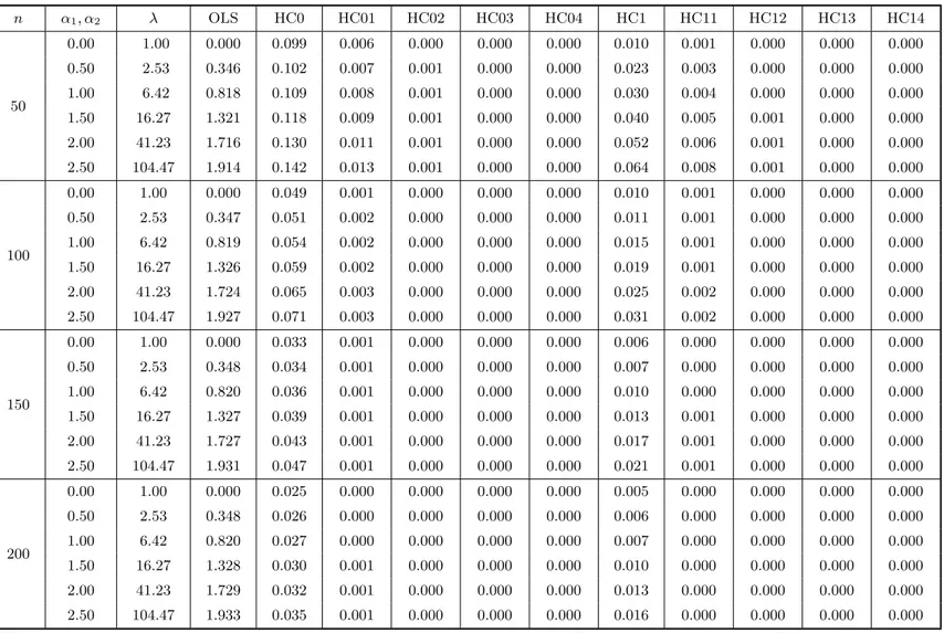
At the outset, Tables 1 and 2 (each divided into two parts, a and b) include the results of the bias evaluation for the OLS, HC0, HC1, HC2 and HC3 variance estimators, and the first four corrected versions of HC0–HC3. Table 1 corresponds to the case where the covariate values were obtained from a uniform distribution, whereas Table 2 relates to the situation where x follows a t3 distribution. In the notation used, HC03, e.g., corresponds to Ψb(3)₀ , i.e., the HC0 (White) estimator corrected up to the third iteration of the bias correcting mechanism. The figures in these tables are the total relative bias of each estimator, which is the sum of absolute relative biases of the variance estimates of βb₁ and βb₂, i.e., it is defined as

|E{var(_c βb₁)} −var(βb₁)|

var(βb1)

+|E{var(c βb2)} −var(βb2)| var(βb2)

,

where ‘var’ denotes the variance estimator of interest. The total relative bias is a measurec of global bias, and the comparisons that follow will be based on this measure. The biases of the unmodified and corrected consistent variance estimators were computed using expression (11). The bias of the usual OLS covariance matrix estimator is given by

tr{Ω(I−H)}

n−p (X

′_X)−1_−PΩP′_,

where here p= 2.

equal to 12% (being equal to 9.9% under homoskedasticity). Third, the HC1 and HC2 estimators outperform the White estimator both under homoskedasticity (in which case the HC2 estimator is unbiased) and heteroskedasticity. The finite-sample performance of the HC2 estimator is slightly better than that of the HC1 estimator. For example, whenn= 150 andλ >1, the maximum total relative bias for HC2 (0.6% forλ = 104.47) is smaller than the minimum total relative bias for HC1 (2.1% forλ = 2.53). Fourth, the HC3 estimator is the unmodified consistent estimator with poorest performance, except under strong heteroskedasticity in which case it outperforms the HC0 estimator.

Fifth, although the individual bias results are not presented (only the total relative biases are presented), we note that the estimator proposed by Halbert White (HC0) always understimated the true variances. This behavior was attenuated by HC1 and HC2 (more effectively by the latter). The HC3 estimator, on the hand, displayed a tendency to overestimate the true variances.

Sixth, it is noteworthy that HC3 is the estimator least sensitive to the degree of heteroskedasticity present in the data. Considering n = 50 and the different values of α1 and α2 used, the difference between the maximum and minimum total relative biases equals 0.005, whereas for the other unmodified consistent estimators this quantity reaches 0.054 (HC1).

Seventh, the biases of the corrected estimators are all very small, even for samples of small size. Note, for instance, that while the total relative bias for HC3 when n = 50 reaches 11%, the total relative bias for the corrected HC3 estimator based on only one iteration does not exceed 0.6%. When n = 200 the corrected estimators display bias values nearly equal to zero, whereas the total relative biases of the HC0 and HC2 estimators are close to 3.5% and 0.5%, respectively.

Table 1a. Bias evaluation I. The model isyt=β1+β2xt+ut, ut∼(0,exp{α1xt+α2x2t}), t= 1, . . . , n. The covariate xt is obtained as random draws from a U(0,1) distribution. The quantities in the table below are the total relative

biases of the HC0 and HC1 estimators and their respective corrected versions, and also the total relative bias of the OLS estimator.

n α1, α2 λ OLS HC0 HC01 HC02 HC03 HC04 HC1 HC11 HC12 HC13 HC14

50

0.00 1.00 0.000 0.099 0.006 0.000 0.000 0.000 0.010 0.001 0.000 0.000 0.000

0.50 2.53 0.346 0.102 0.007 0.001 0.000 0.000 0.023 0.003 0.000 0.000 0.000

1.00 6.42 0.818 0.109 0.008 0.001 0.000 0.000 0.030 0.004 0.000 0.000 0.000

1.50 16.27 1.321 0.118 0.009 0.001 0.000 0.000 0.040 0.005 0.001 0.000 0.000

2.00 41.23 1.716 0.130 0.011 0.001 0.000 0.000 0.052 0.006 0.001 0.000 0.000

2.50 104.47 1.914 0.142 0.013 0.001 0.000 0.000 0.064 0.008 0.001 0.000 0.000

100

0.00 1.00 0.000 0.049 0.001 0.000 0.000 0.000 0.010 0.001 0.000 0.000 0.000

0.50 2.53 0.347 0.051 0.002 0.000 0.000 0.000 0.011 0.001 0.000 0.000 0.000

1.00 6.42 0.819 0.054 0.002 0.000 0.000 0.000 0.015 0.001 0.000 0.000 0.000

1.50 16.27 1.326 0.059 0.002 0.000 0.000 0.000 0.019 0.001 0.000 0.000 0.000

2.00 41.23 1.724 0.065 0.003 0.000 0.000 0.000 0.025 0.002 0.000 0.000 0.000

2.50 104.47 1.927 0.071 0.003 0.000 0.000 0.000 0.031 0.002 0.000 0.000 0.000

150

0.00 1.00 0.000 0.033 0.001 0.000 0.000 0.000 0.006 0.000 0.000 0.000 0.000

0.50 2.53 0.348 0.034 0.001 0.000 0.000 0.000 0.007 0.000 0.000 0.000 0.000

1.00 6.42 0.820 0.036 0.001 0.000 0.000 0.000 0.010 0.000 0.000 0.000 0.000

1.50 16.27 1.327 0.039 0.001 0.000 0.000 0.000 0.013 0.001 0.000 0.000 0.000

2.00 41.23 1.727 0.043 0.001 0.000 0.000 0.000 0.017 0.001 0.000 0.000 0.000

2.50 104.47 1.931 0.047 0.001 0.000 0.000 0.000 0.021 0.001 0.000 0.000 0.000

200

0.00 1.00 0.000 0.025 0.000 0.000 0.000 0.000 0.005 0.000 0.000 0.000 0.000

0.50 2.53 0.348 0.026 0.000 0.000 0.000 0.000 0.006 0.000 0.000 0.000 0.000

1.00 6.42 0.820 0.027 0.000 0.000 0.000 0.000 0.007 0.000 0.000 0.000 0.000

1.50 16.27 1.328 0.030 0.001 0.000 0.000 0.000 0.010 0.000 0.000 0.000 0.000

2.00 41.23 1.729 0.032 0.001 0.000 0.000 0.000 0.013 0.000 0.000 0.000 0.000

Table 1b. Bias evaluation I. The model isyt=β1+β2xt+ut, ut∼(0,exp{α1xt+α2x2t}), t= 1, . . . , n. The covariatext

is obtained as random draws from aU(0,1) distribution. The quantities in the table below are the total relative biases of the HC2 and HC3 estimators and their respective corrected versions.

n α1, α2 λ HC2 HC21 HC22 HC23 HC24 HC3 HC31 HC32 HC33 HC34

50

0.00 1.00 0.000 0.001 0.000 0.000 0.000 0.105 0.005 0.000 0.000 0.000

0.50 2.53 0.005 0.001 0.000 0.000 0.000 0.106 0.005 0.000 0.000 0.000

1.00 6.42 0.011 0.001 0.000 0.000 0.000 0.108 0.005 0.000 0.000 0.000

1.50 16.27 0.016 0.002 0.000 0.000 0.000 0.110 0.006 0.000 0.000 0.000

2.00 41.23 0.018 0.003 0.000 0.000 0.000 0.110 0.006 0.001 0.000 0.000

2.50 104.47 0.020 0.004 0.000 0.000 0.000 0.111 0.006 0.001 0.000 0.000

100

0.00 1.00 0.000 0.000 0.000 0.000 0.000 0.051 0.001 0.000 0.000 0.000

0.50 2.53 0.002 0.000 0.000 0.000 0.000 0.052 0.001 0.000 0.000 0.000

1.00 6.42 0.005 0.000 0.000 0.000 0.000 0.053 0.001 0.000 0.000 0.000

1.50 16.27 0.008 0.000 0.000 0.000 0.000 0.054 0.001 0.000 0.000 0.000

2.00 41.23 0.009 0.001 0.000 0.000 0.000 0.054 0.002 0.000 0.000 0.000

2.50 104.47 0.009 0.001 0.000 0.000 0.000 0.054 0.002 0.000 0.000 0.000

150

0.00 1.00 0.000 0.000 0.000 0.000 0.000 0.034 0.001 0.000 0.000 0.000

0.50 2.53 0.002 0.000 0.000 0.000 0.000 0.034 0.001 0.000 0.000 0.000

1.00 6.42 0.003 0.000 0.000 0.000 0.000 0.035 0.001 0.000 0.000 0.000

1.50 16.27 0.005 0.000 0.000 0.000 0.000 0.035 0.001 0.000 0.000 0.000

2.00 41.23 0.006 0.000 0.000 0.000 0.000 0.036 0.001 0.000 0.000 0.000

2.50 104.47 0.006 0.000 0.000 0.000 0.000 0.036 0.001 0.000 0.000 0.000

200

0.00 1.00 0.000 0.000 0.000 0.000 0.000 0.025 0.000 0.000 0.000 0.000

0.50 2.53 0.001 0.000 0.000 0.000 0.000 0.026 0.000 0.000 0.000 0.000

1.00 6.42 0.003 0.000 0.000 0.000 0.000 0.026 0.000 0.000 0.000 0.000

1.50 16.27 0.004 0.000 0.000 0.000 0.000 0.026 0.000 0.000 0.000 0.000

2.00 41.23 0.004 0.000 0.000 0.000 0.000 0.027 0.000 0.000 0.000 0.000

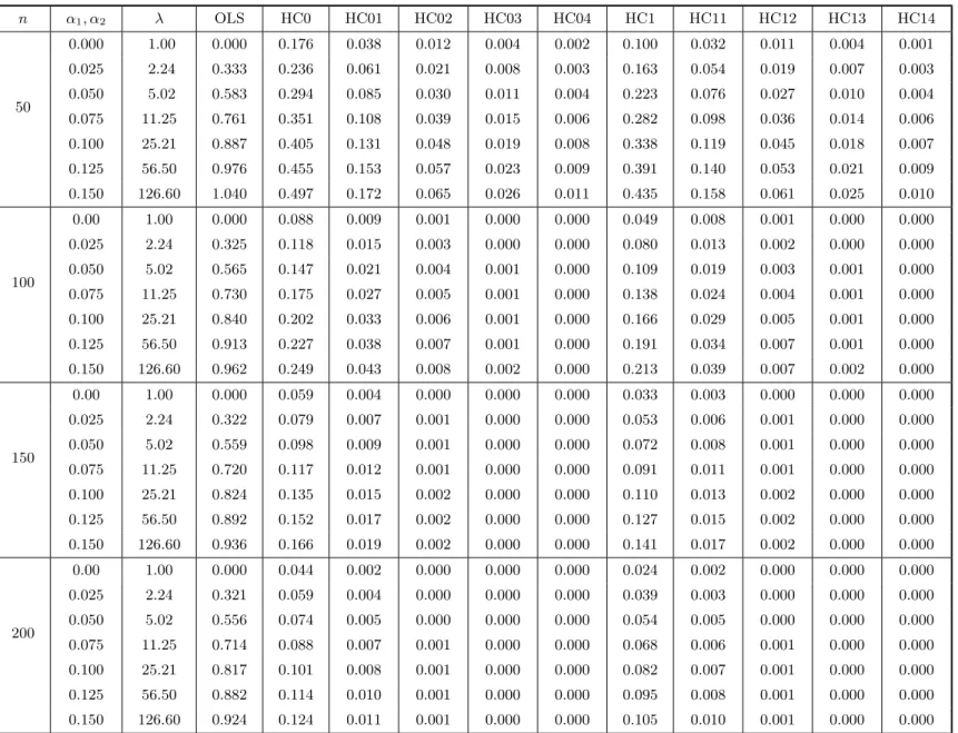
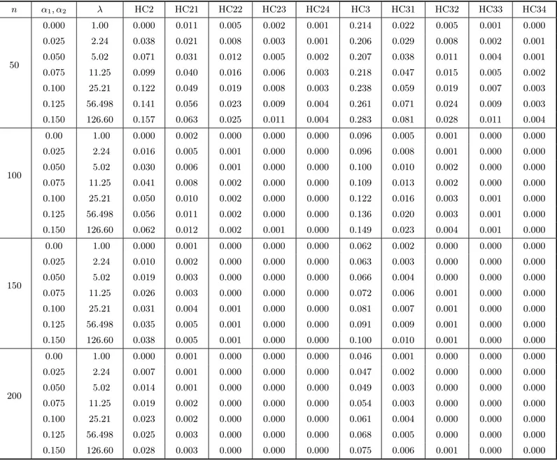
Table 2a. Bias evaluation II. The model isyt=β1+β2xt+ut, ut∼(0,exp{α1xt+α2x2t}), t= 1, . . . , n. The covariatext

is obtained as random draws from at3distribution. The quantities in the table below are the total relative biases of the

HC0 and HC1 estimators and their respective corrected versions, and also the total relative bias of the OLS estimator.

n α1, α2 λ OLS HC0 HC01 HC02 HC03 HC04 HC1 HC11 HC12 HC13 HC14

50

0.000 1.00 0.000 0.176 0.038 0.012 0.004 0.002 0.100 0.032 0.011 0.004 0.001

0.025 2.24 0.333 0.236 0.061 0.021 0.008 0.003 0.163 0.054 0.019 0.007 0.003

0.050 5.02 0.583 0.294 0.085 0.030 0.011 0.004 0.223 0.076 0.027 0.010 0.004

0.075 11.25 0.761 0.351 0.108 0.039 0.015 0.006 0.282 0.098 0.036 0.014 0.006

0.100 25.21 0.887 0.405 0.131 0.048 0.019 0.008 0.338 0.119 0.045 0.018 0.007

0.125 56.50 0.976 0.455 0.153 0.057 0.023 0.009 0.391 0.140 0.053 0.021 0.009

0.150 126.60 1.040 0.497 0.172 0.065 0.026 0.011 0.435 0.158 0.061 0.025 0.010

100

0.00 1.00 0.000 0.088 0.009 0.001 0.000 0.000 0.049 0.008 0.001 0.000 0.000

0.025 2.24 0.325 0.118 0.015 0.003 0.000 0.000 0.080 0.013 0.002 0.000 0.000

0.050 5.02 0.565 0.147 0.021 0.004 0.001 0.000 0.109 0.019 0.003 0.001 0.000

0.075 11.25 0.730 0.175 0.027 0.005 0.001 0.000 0.138 0.024 0.004 0.001 0.000

0.100 25.21 0.840 0.202 0.033 0.006 0.001 0.000 0.166 0.029 0.005 0.001 0.000

0.125 56.50 0.913 0.227 0.038 0.007 0.001 0.000 0.191 0.034 0.007 0.001 0.000

0.150 126.60 0.962 0.249 0.043 0.008 0.002 0.000 0.213 0.039 0.007 0.002 0.000

150

0.00 1.00 0.000 0.059 0.004 0.000 0.000 0.000 0.033 0.003 0.000 0.000 0.000

0.025 2.24 0.322 0.079 0.007 0.001 0.000 0.000 0.053 0.006 0.001 0.000 0.000

0.050 5.02 0.559 0.098 0.009 0.001 0.000 0.000 0.072 0.008 0.001 0.000 0.000

0.075 11.25 0.720 0.117 0.012 0.001 0.000 0.000 0.091 0.011 0.001 0.000 0.000

0.100 25.21 0.824 0.135 0.015 0.002 0.000 0.000 0.110 0.013 0.002 0.000 0.000

0.125 56.50 0.892 0.152 0.017 0.002 0.000 0.000 0.127 0.015 0.002 0.000 0.000

0.150 126.60 0.936 0.166 0.019 0.002 0.000 0.000 0.141 0.017 0.002 0.000 0.000

200

0.00 1.00 0.000 0.044 0.002 0.000 0.000 0.000 0.024 0.002 0.000 0.000 0.000

0.025 2.24 0.321 0.059 0.004 0.000 0.000 0.000 0.039 0.003 0.000 0.000 0.000

0.050 5.02 0.556 0.074 0.005 0.000 0.000 0.000 0.054 0.005 0.000 0.000 0.000

0.075 11.25 0.714 0.088 0.007 0.001 0.000 0.000 0.068 0.006 0.001 0.000 0.000

0.100 25.21 0.817 0.101 0.008 0.001 0.000 0.000 0.082 0.007 0.001 0.000 0.000

0.125 56.50 0.882 0.114 0.010 0.001 0.000 0.000 0.095 0.008 0.001 0.000 0.000

Table 2b. Bias evaluation II. The model isyt=β1+β2xt+ut, ut∼(0,exp{α1xt+α2x2t}), t= 1, . . . , n. The covariate xtis obtained as random draws from at3distribution. The quantities in the table below are the total relative biases of

the HC2 and HC3 estimators and their respective corrected versions.

n α1, α2 λ HC2 HC21 HC22 HC23 HC24 HC3 HC31 HC32 HC33 HC34

50

0.000 1.00 0.000 0.011 0.005 0.002 0.001 0.214 0.022 0.005 0.001 0.000

0.025 2.24 0.038 0.021 0.008 0.003 0.001 0.206 0.029 0.008 0.002 0.001

0.050 5.02 0.071 0.031 0.012 0.005 0.002 0.207 0.038 0.011 0.004 0.001

0.075 11.25 0.099 0.040 0.016 0.006 0.003 0.218 0.047 0.015 0.005 0.002

0.100 25.21 0.122 0.049 0.019 0.008 0.003 0.238 0.059 0.019 0.007 0.003

0.125 56.498 0.141 0.056 0.023 0.009 0.004 0.261 0.071 0.024 0.009 0.003

0.150 126.60 0.157 0.063 0.025 0.011 0.004 0.283 0.081 0.028 0.011 0.004

100

0.00 1.00 0.000 0.002 0.000 0.000 0.000 0.096 0.005 0.001 0.000 0.000

0.025 2.24 0.016 0.005 0.001 0.000 0.000 0.096 0.008 0.001 0.000 0.000

0.050 5.02 0.030 0.006 0.001 0.000 0.000 0.100 0.010 0.002 0.000 0.000

0.075 11.25 0.041 0.008 0.002 0.000 0.000 0.109 0.013 0.002 0.000 0.000

0.100 25.21 0.050 0.010 0.002 0.000 0.000 0.122 0.016 0.003 0.001 0.000

0.125 56.498 0.056 0.011 0.002 0.000 0.000 0.136 0.020 0.003 0.001 0.000

0.150 126.60 0.062 0.012 0.002 0.001 0.000 0.149 0.023 0.004 0.001 0.000

150

0.00 1.00 0.000 0.001 0.000 0.000 0.000 0.062 0.002 0.000 0.000 0.000

0.025 2.24 0.010 0.002 0.000 0.000 0.000 0.063 0.003 0.000 0.000 0.000

0.050 5.02 0.019 0.003 0.000 0.000 0.000 0.066 0.004 0.000 0.000 0.000

0.075 11.25 0.026 0.003 0.000 0.000 0.000 0.072 0.006 0.001 0.000 0.000

0.100 25.21 0.031 0.004 0.001 0.000 0.000 0.081 0.007 0.001 0.000 0.000

0.125 56.498 0.035 0.005 0.001 0.000 0.000 0.091 0.009 0.001 0.000 0.000

0.150 126.60 0.038 0.005 0.001 0.000 0.000 0.100 0.010 0.001 0.000 0.000

200

0.00 1.00 0.000 0.001 0.000 0.000 0.000 0.046 0.001 0.000 0.000 0.000

0.025 2.24 0.007 0.001 0.000 0.000 0.000 0.047 0.002 0.000 0.000 0.000

0.050 5.02 0.014 0.001 0.000 0.000 0.000 0.049 0.003 0.000 0.000 0.000

0.075 11.25 0.019 0.002 0.000 0.000 0.000 0.054 0.003 0.000 0.000 0.000

0.100 25.21 0.023 0.002 0.000 0.000 0.000 0.061 0.004 0.000 0.000 0.000

0.125 56.498 0.025 0.003 0.000 0.000 0.000 0.068 0.005 0.000 0.000 0.000

A quick comparison between Tables 1 and 2 indicate that the presence of high leverage points in the data is more decisive to the reliability of the different covariance matrix estimators than the degree of heteroskedasticity itself. For example, whenn = 50 and the design matrix does not contain high leverage points the total relative biases of the consistent estimators understrong heteroskedasticity are smaller than the respective biases in the situation where there are leverage points and the data are homoskedastic. It is possible to identify the presence of high leverage points in the second design by looking atht,t= 1, . . . , n, the diagonal elements ofH. It can be shown that 0< ht<1 for all t. Note also that Pn_t=1ht = tr(H) = tr[X(X′X)−1X′] = p. The ht’s therefore have an average value of p/n. A general rule–of–thumb is that values of ht in excess of two or three times the average are regarded as influential and worthy of further investigation (Judge et al., 1988, p. 893). As noted by Chesher & Jewitt (1987, p. 1219), the possibility of severe downward bias in the White estimator arises when there are largeht, because the associated least squares residuals have small magnitude on average and the White estimator takes small residuals as evidence of small error variances.

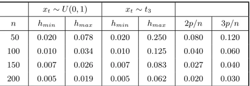
Table 3 displays the maximum and minimum values of ht for the two regression designs under consideration; it also includes the benchmark values of 2p/n and 3p/n. We note that when the covariate values are obtained from at3 distribution the maximum value of ht exceeds 3p/n, thus suggesting that the data contain potentially influential observations. The same does not happen when the covariate values are obtained from a uniform distribution, in which case the design matrix contains no leverage point.

Table 3. Identification of high leverage points.

xt∼U(0,1) xt∼t3

n hmin hmax hmin hmax 2p/n 3p/n

50 0.020 0.078 0.020 0.250 0.080 0.120

100 0.010 0.034 0.010 0.125 0.040 0.060

150 0.007 0.026 0.007 0.083 0.027 0.040

200 0.005 0.019 0.005 0.062 0.020 0.030

Variance estimators of different linear combinations of the ordinary least squares estimator are affected differently by the heteroskedasticity present in the data. We shall now determine the linear combination of the regression parameter estimators that yields the maximal estimated variance bias, that is the p-vectorcsuch that c′_{c= 1 and}

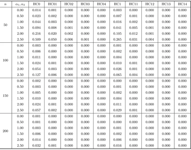
E{var(_c c′βb)}−var(c′βb) is maximized. Since the bias matrices given in (11) are symmetric, the maximum absolute value of the bias of the estimated variances of linear combinations of theβb’s is the maximum of the absolute values of the eigenvalues of the corresponding bias matrices. The results are presented in Table 4 (which is divided into 4a and 4b) for the case where the covariate values are obtained from a uniform distribution.

Table 4a. Bias evaluation III. The entries in the table below are the absolute value of the maximal bias of

c

var(c′_βb_{) for different variance estimators.}

n α1, α2 HC0 HC01 HC02 HC03 HC04 HC1 HC11 HC12 HC13 HC14

50

0.00 0.014 0.001 0.000 0.000 0.000 0.003 0.000 0.000 0.000 0.000

0.50 0.023 0.002 0.000 0.000 0.000 0.007 0.001 0.000 0.000 0.000

1.00 0.044 0.003 0.000 0.000 0.000 0.016 0.002 0.000 0.000 0.000

1.50 0.094 0.008 0.001 0.000 0.000 0.041 0.005 0.001 0.000 0.000

2.00 0.216 0.020 0.002 0.000 0.000 0.105 0.012 0.001 0.000 0.000

2.50 0.509 0.050 0.006 0.001 0.000 0.265 0.031 0.004 0.000 0.000

100

0.00 0.003 0.000 0.000 0.000 0.000 0.001 0.000 0.000 0.000 0.000

0.50 0.006 0.000 0.000 0.000 0.000 0.002 0.000 0.000 0.000 0.000

1.00 0.011 0.000 0.000 0.000 0.000 0.004 0.000 0.000 0.000 0.000

1.50 0.024 0.001 0.000 0.000 0.000 0.010 0.001 0.000 0.000 0.000

2.00 0.054 0.003 0.000 0.000 0.000 0.026 0.001 0.000 0.000 0.000

2.50 0.127 0.006 0.000 0.000 0.000 0.065 0.004 0.000 0.000 0.000

150

0.00 0.002 0.000 0.000 0.000 0.000 0.000 0.000 0.000 0.000 0.000

0.50 0.003 0.000 0.000 0.000 0.000 0.001 0.000 0.000 0.000 0.000

1.00 0.005 0.000 0.000 0.000 0.000 0.002 0.000 0.000 0.000 0.000

1.50 0.010 0.000 0.000 0.000 0.000 0.004 0.000 0.000 0.000 0.000

2.00 0.024 0.001 0.000 0.000 0.000 0.011 0.000 0.000 0.000 0.000

2.50 0.057 0.002 0.000 0.000 0.000 0.029 0.001 0.000 0.000 0.000

200

0.00 0.001 0.000 0.000 0.000 0.000 0.000 0.000 0.000 0.000 0.000

0.50 0.001 0.000 0.000 0.000 0.000 0.000 0.000 0.000 0.000 0.000

1.00 0.003 0.000 0.000 0.000 0.000 0.001 0.000 0.000 0.000 0.000

1.50 0.006 0.000 0.000 0.000 0.000 0.002 0.000 0.000 0.000 0.000

2.00 0.014 0.000 0.000 0.000 0.000 0.006 0.000 0.000 0.000 0.000

Table 4b. Bias evaluation III. The entries in the table below are the absolute value of the maximal bias of

c

var(c′_βb_{) for different variance estimators.}

n α1, α2 HC2 HC21 HC22 HC23 HC24 HC3 HC31 HC32 HC33 HC34

50

0.00 0.000 0.000 0.000 0.000 0.000 0.015 0.001 0.000 0.000 0.000

0.50 0.001 0.000 0.000 0.000 0.000 0.022 0.001 0.000 0.000 0.000

1.00 0.005 0.001 0.000 0.000 0.000 0.037 0.002 0.000 0.000 0.000

1.50 0.015 0.002 0.000 0.000 0.000 0.069 0.004 0.000 0.000 0.000

2.00 0.045 0.006 0.001 0.000 0.000 0.139 0.009 0.001 0.000 0.000

2.50 0.121 0.016 0.002 0.001 0.000 0.295 0.020 0.002 0.000 0.000

100

0.00 0.000 0.000 0.000 0.000 0.000 0.004 0.000 0.000 0.000 0.000

0.50 0.000 0.000 0.000 0.000 0.000 0.005 0.000 0.000 0.000 0.000

1.00 0.001 0.000 0.000 0.000 0.000 0.009 0.000 0.000 0.000 0.000

1.50 0.004 0.000 0.000 0.000 0.000 0.017 0.001 0.000 0.000 0.000

2.00 0.011 0.001 0.000 0.000 0.000 0.034 0.001 0.000 0.000 0.000

2.50 0.029 0.002 0.000 0.000 0.000 0.073 0.003 0.000 0.000 0.000

150

0.00 0.000 0.000 0.000 0.000 0.000 0.002 0.000 0.000 0.000 0.000

0.50 0.000 0.000 0.000 0.000 0.000 0.002 0.000 0.000 0.000 0.000

1.00 0.000 0.000 0.000 0.000 0.000 0.004 0.000 0.000 0.000 0.000

1.50 0.002 0.000 0.000 0.000 0.000 0.007 0.000 0.000 0.000 0.000

2.00 0.005 0.000 0.000 0.000 0.000 0.015 0.000 0.000 0.000 0.000

2.50 0.013 0.001 0.000 0.000 0.000 0.032 0.001 0.000 0.000 0.000

200

0.00 0.000 0.000 0.000 0.000 0.000 0.001 0.000 0.000 0.000 0.000

0.50 0.000 0.000 0.000 0.000 0.000 0.001 0.000 0.000 0.000 0.000

1.00 0.000 0.000 0.000 0.000 0.000 0.002 0.000 0.000 0.000 0.000

1.50 0.001 0.000 0.000 0.000 0.000 0.004 0.000 0.000 0.000 0.000

2.00 0.003 0.000 0.000 0.000 0.000 0.008 0.000 0.000 0.000 0.000

HC3. Under homoskedasticity, HC0 and HC3 have approximately the same finite-sample behavior, and HC3 outperforms HC0 under unequal error variances. It is noteworthy that the maximal biases are always much larger for the unmodified estimators than for their respective corrected versions. For n = 50 and α1 = α2 = 2.50, for instance, we obtain maximal biases for the one-iteration corrected estimators that are 10 times smaller than those of the respective original estimators.

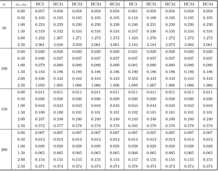
In order to evaluate the variances of the different variance estimators of linear com-binations of the elements of βbwe use the exact expression given in (20). The results for uniform covariate values and c= (0,1)′ are given in Table 5 (again divided into 5a and 5b). The entries correspond to the standard errors of the estimators of var(βb2). It is well known that bias correction oftentimes induces variance inflation, and we note that this occurs here. It is important to note, however, that the variance inflation induced by the bias correction mechanism is not large, especially when heteroskedasticity is not strong. For example, when n= 50 and α1 =α2 = 1.00 (λ= 6.42), the standard errors of the HC0 estimator and its first four corrected versions are, respectively, 0.209, 0.228, 0.230, 0.230, 0.230. Two remarks are in order here: 1) The bias correction mechanism reduces the variance of the estimator when applied to HC3, conversely to what happens to ther estimators. 2) From the third iteration of the bias correcting mechanism on, the variances of the improved estimators become stable.

5. Concluding remarks

Cross sectional data oftentimes display some form of heteroskedasticity. It is common practice to still use the OLSE of the vector of regression parameters, since it remains unbiased and consistent. Its covariance matrix, however, has to be consistently esti-mated in order for inference to be performed. In this paper, we propose a sequence of bias adjusted heteroskedasticity-consistent covariance matrix estimators. The sequence of improved estimators is defined by sequentially transforming a selected consistent es-timator. The proposed sequence is general enough to be applicable to a number of well known estimators. Overall, the numerical results favor improved estimators obtaining by modifying the HC2 heteroskedasticity-consistent covariance matrix estimator.

Acknowledgements

Table 5a. Variance evaluation. The entries in the table below are the standard error of the different variance estimators for the OLS slope estimator in a simple linear regression model.

n α1, α2 HC0 HC01 HC02 HC03 HC04 HC1 HC11 HC12 HC13 HC14

50

0.00 0.054 0.058 0.058 0.058 0.058 0.056 0.058 0.058 0.058 0.058

0.50 0.097 0.105 0.105 0.105 0.105 0.101 0.105 0.105 0.105 0.105

1.00 0.209 0.228 0.230 0.230 0.230 0.218 0.228 0.230 0.230 0.230

1.50 0.484 0.529 0.534 0.534 0.534 0.504 0.531 0.534 0.534 0.534

2.00 1.148 1.258 1.270 1.272 1.272 1.195 1.262 1.271 1.272 1.272

2.50 2.754 3.026 3.057 3.060 3.061 2.869 3.037 3.058 3.061 3.061

100

0.00 0.019 0.020 0.020 0.020 0.020 0.020 0.020 0.020 0.020 0.020

0.50 0.035 0.036 0.037 0.037 0.037 0.036 0.037 0.037 0.037 0.037

1.00 0.076 0.080 0.080 0.080 0.080 0.078 0.080 0.080 0.080 0.080

1.50 0.177 0.185 0.186 0.186 0.186 0.181 0.185 0.186 0.186 0.186

2.00 0.421 0.441 0.442 0.443 0.443 0.430 0.442 0.442 0.443 0.443

2.50 1.013 1.063 1.066 1.066 1.066 1.034 1.064 1.066 1.066 1.066

150

0.00 0.011 0.011 0.011 0.011 0.011 0.011 0.011 0.011 0.011 0.011

0.50 0.019 0.020 0.020 0.020 0.020 0.019 0.020 0.020 0.020 0.020

1.00 0.042 0.043 0.043 0.043 0.043 0.042 0.043 0.043 0.043 0.043

1.50 0.097 0.100 0.101 0.101 0.101 0.099 0.100 0.101 0.101 0.101

2.00 0.232 0.239 0.240 0.240 0.240 0.235 0.239 0.240 0.240 0.240

2.50 0.558 0.577 0.578 0.578 0.578 0.566 0.577 0.578 0.578 0.578

200

0.00 0.007 0.007 0.007 0.007 0.007 0.007 0.007 0.007 0.007 0.007

0.50 0.013 0.013 0.013 0.013 0.013 0.013 0.013 0.013 0.013 0.013

1.00 0.027 0.028 0.028 0.028 0.028 0.028 0.028 0.028 0.028 0.028

1.50 0.064 0.065 0.065 0.065 0.065 0.064 0.065 0.065 0.065 0.065

2.00 0.151 0.155 0.155 0.155 0.155 0.153 0.155 0.155 0.155 0.155

Table 5b. Variance evaluation. The entries in the table below are the standard error of the different variance estimators for the OLS slope estimator in a simple linear regression model.

n α1, α2 HC2 HC21 HC22 HC23 HC24 HC3 HC31 HC32 HC33 HC34

50

0.00 0.057 0.058 0.058 0.058 0.058 0.061 0.058 0.058 0.058 0.058

0.50 0.103 0.105 0.105 0.105 0.105 0.110 0.106 0.105 0.105 0.105

1.00 0.224 0.229 0.230 0.230 0.230 0.240 0.231 0.230 0.230 0.230

1.50 0.519 0.532 0.534 0.534 0.534 0.557 0.536 0.535 0.534 0.534

2.00 1.232 1.267 1.271 1.272 1.272 1.323 1.276 1.272 1.272 1.272

2.50 2.961 3.048 3.059 3.061 3.061 3.184 3.184 3.072 3.062 3.061

100

0.00 0.020 0.020 0.020 0.020 0.020 0.021 0.020 0.020 0.020 0.020

0.50 0.036 0.037 0.037 0.037 0.037 0.037 0.037 0.037 0.037 0.037

1.00 0.079 0.080 0.080 0.080 0.080 0.081 0.080 0.080 0.080 0.080

1.50 0.183 0.186 0.186 0.186 0.186 0.190 0.186 0.186 0.186 0.186

2.00 0.436 0.442 0.442 0.443 0.443 0.452 0.443 0.443 0.443 0.443

2.50 1.050 1.065 1.066 1.066 1.066 1.088 1.067 1.066 1.066 1.066

150

0.00 0.011 0.011 0.011 0.011 0.011 0.011 0.011 0.011 0.011 0.011

0.50 0.020 0.020 0.020 0.020 0.020 0.020 0.020 0.020 0.020 0.020

1.00 0.043 0.043 0.043 0.043 0.043 0.044 0.043 0.043 0.043 0.043

1.50 0.100 0.100 0.101 0.101 0.101 0.102 0.101 0.101 0.101 0.101

2.00 0.237 0.240 0.240 0.240 0.240 0.243 0.240 0.240 0.240 0.240

2.50 0.572 0.577 0.578 0.578 0.578 0.585 0.578 0.578 0.578 0.578

200

0.00 0.007 0.007 0.007 0.007 0.007 0.007 0.007 0.007 0.007 0.007

0.50 0.013 0.013 0.013 0.013 0.013 0.013 0.013 0.013 0.013 0.013

1.00 0.028 0.028 0.028 0.028 0.028 0.028 0.028 0.028 0.028 0.028

1.50 0.065 0.065 0.065 0.065 0.065 0.066 0.065 0.065 0.065 0.065

2.00 0.154 0.155 0.155 0.155 0.155 0.157 0.155 0.155 0.155 0.155

References

[1] Chesher, A. & Jewitt, I. (1987). The bias of a heteroskedasticity consistent covariance matrix estimator. Econometrica, 55, 1217–1222.

[2] Cribari–Neto, F., Ferrari, S.L.P. & Cordeiro, G.M. (2000). Improved heteroscedasticity–consistent covariance matrix estimators. Biometrika, 87, 907–918.

[3] Cribari–Neto, F. & Zarkos, S.G. (1999). Bootstrap methods for heteroskedastic regression models: evidence on estimation and testing. Econometric Reviews, 18, 211–228.

[4] Doornik, J.A. (2001). Ox: an Object–oriented Matrix Programming Language, 4th ed. London: Timberlake Consultants & Oxford: http://www.nuff.ox.ac.uk/Users/Doornik.

[5] Hinkley, D.V. (1977). Jackknifing in unbalanced situations. Technometrics, 19, 285–292.

[6] Horn, S.D., Horn, R.A. & Duncan, D.B. (1975). Estimating heteroskedastic variances in linear models. Journal of the American Statistical Association, 70, 380–385.

[7] Judge, G.C, Hill, R.C., Griffiths, W.E., Lutkepohl, H. & Lee, T.C. (1988). Introduction to the Theory and Pratice of Econometrics, 2nd ed. New York: Wiley.

[8] Long, J.S. & Ervin, L.H. (2000). Using heteroskedasticity-consistent standard errors in the linear regression model. The American Statistician, 54, 217–224.

[9] MacKinnon, J.G. & White, H. (1985). Some heteroskedasticity-consistent covariance matrix esti-mators with improved finite-sample properties. Journal of Econometrics, 29, 305–25.

[10] Rao, C.R. (1973). Linear Statistical Inference and its Applications, 2nd ed. New York: Wiley. [11] Seber, G.A.F. (1977). Linear Regression Analisys. New York: Wiley.