The Use of Semi-parametric Methods in Achieving Robust Inference

r

.

.

.

'

j~.

i

'~

_~

I

I

'

i

_·~

;;

~

~

-~

_•

i

.i

~

!

~

~

J

1

~

-~~

~

~

l

I

I

·.\

The

Use

of Semi-parametric Methods in Achieving

Robust Inference

Jose Manuel de Matos Passos

A thesis submitted to the University of Bristol in accordance with the

requirements for the degree of Ph,D. in the Faculty of Social Sciences,

Department of Economics

May 1996

·.,,

·---e--lk,; o ·,, , -;-~. I ' ' '

-t

ti

n

tl

h

pt

m

th

as:

he1

to

/',

' ' .

\'I\

\

~ .. ;·:. '::.

ABSTRACT

This thesis focuses on some topics in semi-parametric econometrics, particularly

the use of semi-parametric methods of estimation to obtain robust inference.

Chapter two proposes a study of the finite-sample performance of the

heteroskedas-tic and autocorrelation consistent covariance matrix estimators (HAC). This

perfor-mance is accessed through the bias of the first moment of HAC type estimators and

the quality of the asymptotic normal approximation to the exact finite-sample

distri-butions of HAC type Wald statistics of scalar linear hypothesis.

In Chapter three, the use of the non-overlapping deleted-l jackknife is used to

pro-pose a new approach to estimate the covariance matrix of the least square estimator

in a linear regression model. This estimator is robust to the presence of

heteroskedas-tldty and autocorrelation in the errors.

Chapter four deals with improved estimation of regression coefficients through an

alternative and efficient method of estimation regression models under

heteroskedas-ticity of tmknown form. Kernel and average derivative estimation are used to estimate

the conditional variance of the response variable where this conditional variance is

assumed to be in an index form.

Chapter five is concerned with the estimation of duration models under unobserved

heterogeneity. This is a typical problem in mlcroer.onometrics and is in general due

to differences among individuals. It is suggested a method of estimation based on a

roughness penalty approach.

ACKNOWLEDGEMENTS

I am deeply indebted to my supervisor Andrew Chesher for his support and

guid-ance that made this work possible.

I also would like to thank Whitney Newey, Bernard Silverman, Roger Klein, Garry

Phillips and Oliver Linton for helpful comments on several parts of the thesis.

This work would not have been possible without the three years leave kindly granted

by the Departamento de Matematica do lnstituto Superior de Economia e Gestao

(ISEG) da Universidade Tecnica de Lisboa. I am also grateful to my colleague Joao

Santos Silva, my M.Sc. supervisor Bento Murteira and to the President of the

Sci-entific Council of ISEG Carlos da Silva Ribeiro for their friendship, support and

encouragement.

Financial support from Banco de Portugal postgraduate scholarship fund is

grate-fully acknowledged. Without it this work would not have been possible.

Finally, a very special thank to my wife Helena and my son Ricardo for their

AUTHOR'S DECLARATION

The work presented in this thesis was carried out in the Department of Economics

at the University of Bristol and it is entirely my own.

The views expressed in this thesis are those of the author and not of the University

of Bristol.

(

_'il

Chapter 1

CONTENTS

An Overview

1. The use of semi-parametric methods in achieving robust

inference

2. References

Chapter 2 - Finite-Sample Performance of the Heteroskedasticity

and Autocorrelation Consistent Covariance Matrix

Estimators

1. Introduction

2. HAC Type Estimators in the Linear Model

3. Moments of the HAC Estimators

4. Bias of the HAC Estimators

4.1. Choice of the lag truncation

4.2. Independent and Homoeskedastk Errors

4.3. Non-independent and Homoeskedastk Errors

4.4. Modified Newey and West Estimator

5. The Finite-Sample Distributions of Heteroskedasticity

and Autocorrelation Robust Wald Statistic

6. Concluding Remarks

7. References

1

1

6

'7

7

9

13

14

17

20

25

28

29

58

Chapter 3 - Heteroskedasticity and Autocorrelation Consistent

Covariance Matrix Estimator with Improved

Finite-Sample Properties: an approach based on a group

Jackknife estimator.

1. Introduction

2. Notation and Estimator

3.

First Moment of the Grouped Jackknife Estimator of

the Variance

4. Application

5. Further Comments

6. Appendix

7.

References

Chapter 4 - Adapting for heteroskedasticity of unknown form:

An Approach via ADE

1. Introduction 2. The Estimator

3. Testing the Heteroskedastidty and the Variance

Assumption

4. Application

5. Concluding Remarks

6. References

63

63

65

69

70

78

79

90

92

92

94

104

106

115

Chapter 5 Estimation of Duration Models with Unobserved

Heterogeneity: a roughness penalty approach 118

1. Introduction 118

2.

Model and Estimator

122

3. Application

130

4. Furt.her Comments and Conclusions

142

CHAPTER 1 - AN OVERVIEW

1. THE USE OF SEMI-PARAMETRIC METHODS IN ACHIEVING

ROBUST INFERENCE.

This thesis focuses on some topics in semi-parametric econometric~, particularly

the application of semi-parametric methods of estimation to obtain robust inference.

It is a relatively wide area, including a large variety of econometric work and a

de-tailed and comprehensive study of this subject is clearly beyond the scope of this

thesis. Only some topics will be addressed here.

Traditionaly, the statistical analysis of economic data is based on a specification

of a parametric model depending on a finite number of unknown parameters. This

parametric model is usually described as a functional relation between a dependent

variable, y, and a set of observable covariates, x, and an unobservable error, c:, where

y = g(x,B,c:), ()is an unknown parameter and g(.) is a known function. For this

specification to be completed the parametric approach specifies the distribution of

the error term. With these elements in hand, the maximum likelihood method can

be applied to the estimation of B. If the model is correctly specified, it is well known

that the maximum likelihood estimator (m.l.e.) has all desirable properties as

However this framework has its limitations and can be misleading if not applied

carefully. The literature is rich with examples concerning the consequences of

depar-tures from the initial assumptions about the parametric model considered. This can

lead to incorrect variance estimates or even inconsistency of the estimator. If some

of the initial assumptions fails or can not be assumed or if there are components

of the model that can not be parameterized, the semi-parametric approach appears

as a valuable instrument [for a survey in semi-parametric methods in econometrics

consider for example Robinson (1988) and Powell (1992)].

This thesis is concerned with the application of semi-parametric methods in two

situations: misspecification of the assumptions concerning the error term as the

in-dep~ndence and identically distributed (i.i.d) assumption and misspecification of the

model by neglecting heterogeneity, in the context of duration models. The purpose is

to use semi-parametric methods in order to make inferences that are robust to these

problems. Chapters two to four address the first problem and chapter five addresses

the second.

Most of these chapters were originally developed as discussion papers and essays

that have been organized in order to produce the five chapters of this thesis, where

each one is self contained and independent of the others.

Both mkroeconomic and macroeconomic. data present characteristics that can

con-tribute to violate the assumption of i.i.d. errors. The reasons are heterogeneous

pop-ulation in the first case and temporal dependency in the latter. It is well known that

under these circumstances, the usual least square estimator is still consistent but the

standard errors are incorrectly estimated. For this reason and because the pattern

of the errors are unknown, the traditional procedure is to correct the standard errors

the literature, the estimator proposed in Newey and West (1987) has been suggested.

However there is a lack of knowledge concerning its finite-simple properties and this

problem will be studied here.

Chapter two is concerned with the study of the Heteroskedasticity and

Autocorrela-tion Consistent Covariance Matrix (HAC) estimators for the least-squares regression

coefficients. Among the HAC type estimators the Newey and West (1987) estimator

is considered to show the relation between its finite-sample performance and the

de-sign generated by the regressors. This performance is assessed through the bias of

the first moment of HAC type estimators and the quality of the asymptotic normal

approximation to the exact finite-sample distributions of HAC type Wald statistics

of scalar linear hypothesis. In this case Imhof procedure is used. A slight

modifi-cation of the Newey and West estimator, based on a bias correction in the case of

homoskedast.ic and non-ant.ocorrelated errors, is also presented.

The recent development in non-parametric and semi-parametric methods of

estima-tion opened the way to a growing research in econometrics. Having in mind these new

resources and the fact that HAC estimators can be severely biased in small samples, a

rather different approach is suggested. The deleted-l Jackknife with non-overlapping

blocks and Average Derivative Estimation techniques are used in chapter three and

four respectively to develop estimators that are robust to heteroskedasticity and/ or

autocorrelation in the error term. These estimators can be viewed as alternatives and

generalizations of some estimators presented in the literature.

In part. three it is proposed a new approach to estimating the covariance matrix of the least square (henceforth LS) estimator in a linear regression model. This

ap-proach was inspired by a previous paper of Carlstein (1986) concerning the use of

subseries values for estimating the variance of a sample mean, based on dependent

the LS estimator in regression models. To deal with it and to avoid problems related

to a possible lack of degrees of freedom, the non-overlapping deleted-l jackknife (or

grouped jackknife) is used instead. This estimator is robust to the presence of

het-eroskedastidty and autocorrelation in the errors. In another way it generalizes the

heteroskedasticity consistent covariance matrix estimator (or the deleted-1 jackknife

estimator, as is it known in the literature), to situations with non-independent

sta-tionary errors. It is also an alternate to the estimator presented by Newey and West

(1987). An application concerning the finite-sample performance of this estimator is

also presented.

Chapter four deals with improved estimation of regression coefficients through an

alternative and efficient method of estimation regression models under

heteroskedas-ticity of unknown form. In this case, the pattern of heteroskedasheteroskedas-ticity is first

esti-mated non-parametrically and then used as weights via weighted (non-linear) least

square estimation. Kernel smoothing and average derivative estimation (henceforth

ADE) will be used to estimate the conditional variance of the response variable, where

this conditional variance is assumed to be in an index form. This method is presented

as a generalisation of Carrol's (1982) estimator where the conditional variance of the

response variable is not restricted to be a function of the conditional mean of the

response variable. A comparison is made through a Monte Carlo simulation.

Chapter five is concerned with the estimation of duration models when

unobserv-able individual effects are present. This problem can be viewed as a mixture model

where the density of the unobservables is the unknown mixing density that is to be

estimated using some appropriated method. Two different approaches have been

con-sidered in the literature: one uses a parametric specification of the heterogeneity by

assuming some mixing density; the other one uses nonparametric methods as, for

ex-ample, the non-parametric maximum likelihood estimation. The first approach is too

the underlying mixing density is poorly estimated. In this chapter it is suggested an

2. REFERENCES

Carlstein, E. (1986). The use of subseries values for estimating the variance of

a general statistic from a stationary sequence, The Annals of Statistics, 14,

1171-1179.

Carrol, R. J. (1982). Adapting for Heteroskedasticity in Linear Models. Annals

od Statistics, 10, 1224-1233.

Newey, W. and West, K. (1987). A Simple, Positive Semi-Definite,

Het-eroskedasticity and Autocorrelation Consistent Covariance Matrix,

Economet-rica., 55, 703-708.

Powell, J. (1992). Estimation of Semiparametric Models. Draft, Princeton

Uni-versity.

Robinson, P. (1988). Semiparametric Econometrics: A Survey. Journal of

CHAPTER 2 - FINITE-SAMPLE PERFORMANCE OF THE

HETEROSKEDASTICITY AND AUTOCORRELATION

CONSISTENT COVARIANCE MATRIX ESTIMATORS

1.

INTRODUCTION

In the econometric framework, the consequences of autocorrelated and

heteroskedas-tic errors have been studied in the literature for a long time. These are common

prob-lems associated with time series and cross sectional models, respectively, as it can be

seen when some useful diagnostic tests are applied. In this context it is well lmown

that if the errors are heteroskedastic and/ or autocorrelated, the usual estimator is

still consistent but the standard errors are erroneous.

If the form of autocorrelation and/or heteroskedasticity is known, there are

appro-priated techniques to minimise this problem. However this is not what happens in

general and several works have been developed to find a consistent estimator of the

standard errors, robust to this kind of unlmown error structure.

The key to finding such an estimator is due to Eicker (1963). He has shown in the

case of heteroskedasticity of unknown order, that consistent estimation of the

covari-ance matrix estimator of the least-squares (LS) regression coefficients does not require

consistent estimation of the variance of the disturbance term. White (1980),

heteroskedasticity consistent covariance matrix (henceforth HCCM) estimators. But

when the errors are not independent other estimators will be needed. In a pioneering

paper concerning Generalised Method of Moments estimation Hansen (1982) derived

a heteroskedasticity and autocorrelation consistent covariance (henceforth HAC)

es-timator. Since then several works have addressed this subject. Hansen and Singleton

{1982), have applied this estimator in a non-linear rational expectations model; White

(1984) dedicated a whole chapter to studying the properties of Hansen's type

esti-mator for different structures of the errors; White and Domowitz (1984) applied this

estimator to the non-linear regression; Wooldridge (1991) suggest the use of this

estimator in robust diagnostics for non-linear models of conditional means and

con-ditional variance; Newey and West (1987) presented a positive semi-definite matrix

estimator; Andrews {1991) showed that all these estimators can be viewed as

ker-nel esti~ators, presenting simultaneously a Monte Carlo study for different types of

kernels. Moreover he advocates an HAC estimator that uses the Quadratic-Spectral

kernel. In this context the estimators proposed by Hansen (1982) [see also White

(1984)], Newey and West (1987) and Gallant (1987, pag. 533) correspond to

estima-tors using truncated, Bartlett and Parzen kernels, respectively. Recently, Andrews

and Monahan (1992) proposed a slightly different version and named it prewhitened

kernel estimator, with vector autoregressions employed in the prewhitening stage.

When one suspects for non-iid errors and little is known about their structure, the

use of HAC type estimators in test statistics have been suggested by the authors

being cited as a way to compute correct standard errors and therefore correct

infer-ences. Furthermore its facility of computation is now accessable through econometric

packages like Shazam. However little is known about their finite-sample properties.

In a previous paper, Chesher and Jewitt (1987) developed finite-sample results for

the HCCM estimators, showing that substantial bias can occur when the regression

design contains points of high leverage. In what follows their results are extended to

The remainder of this Chapter is organised as follows. In Section 2, are presented

the HAC type estimators (in particular the Newey and West estimator) and some

notation related to them, in the context of linear models. Additionally it is shown

that HAC type estimators can be decomposed in a HCCM estimator and in an

Au-tocorrelation Consistent Covariance estimator. The expectation and variance of this

estimator are presented in Section 3. Section 4 is dedicated to the finite-sample

per-formance of the Newey and West estimator, given particular attention to the effects of

leverage points in the data. In this context three different error structures are

consid-ered: independent, AR(l) and MA(l) errors. Section 5 is dedicated to the evaluation

~ of the quality of the first-order asymptotic approximation to the null distribution of

11

the Wald test, using the Newey and West estimator. Finally, Section 6 summarises

I!

1! the main conclusions and presents some possible directions for future research.

li

2. HAC TYPE ESTIMATORS IN THE LINEAR MODEL

The present work deals with the linear model,

y =

X(3

+

c, (1)

where y is ann X 1 vector of observations, X is an X k matrix of full column rank k

with rows xi, f-1 is a kx1 vector of unknown parameters and cis an X 1 vector of errors

with E(c

I

X)=

0 and E(cc1

I

_X)=

n

_{positive definite of order n X n. Additionally}

it is assumed that, conditional on X, the errors are covariance stationary. Under

these assumptions, the covariance matrix of the LS estimator of

(3,

fJ

=

(X'

X)-1

X'y,

In this expression X'OX can be decomposed in a suitable way by,

n n-1 n

X' OX=

L:

7(0)

x~xi+

L: L:

7(j)

(x~xi-J

+

:v~_Jxi) , (3)

i=O j=li=j+l

where "((j) =

E(cici-j)

is the autocovariance function of order j and

"f(O)

the error variance that is assumed constant from now on.

In the LS context, the direct estimation of

n,

substituting the unknown errors, Ei,

by the residuals, E.i, leads to a degenerate estimator, due to the orthogonality

condi-tion, X'€ = 0. If the errors are covariance stationary, the autocovariance function,

E(ci€j), is a function of the difference,

I

i -j

I·

Additionally if one limits the attention

to the case in which the autocovariance function of order

I

i - j

I

decreases as

I

i - j

I

tends to infinity, it seems reasonable to estimate X'OX considering only the most

significant autocovariances. In the particular case of linear models, Hansen's (1982)

estimator can be expressed as follows,

n m n

X'

OX

=

L ~ x~xi+

L L

fifi_J(x~xi-J

+

x~_Jxi)

,

(4)

i=O j=li=j+l

where m is a lag truncation that in general equals the number of non-zero

auto-correlations of :<ci· If the structure of the errors is known a priori, for example if

it is a moving average of order q, then such lag should be equal to q. When this

ap-propriated methods to choose the optimal value of m. However Hansen's estimator

has the drawback of not always being positive semi-definite. To solve this problem,

two techniques have been usually presented in the literature: time domain techniques

due to Cumby, Huizinga and Obstfeld (1983) and Newey and West (1987), among

others, and frequency domain techniques suggested initially by Hansen (1982) and

adopted later by Andrews (1991, 1992)1_{• In what follows time the domain technique}

is considered, particularly the Newey and West estimator due to its simplicity of

com-putation. These authors proposed a positive semi-definite HAC estimator, simply by

smoothing the samples autocovariances in ( 4),

n m n

X'

OX=

L

4

x~xi+

L L

~(j,

m)

ei€i-j

(x~Xi-J'

+

x~-jxi),

(5)

i=O i=li=j+l

where

K(j,

m) = 1- j ,

m+1

(6)

is the weight associated with the autocovariance of order j (Having in mind the

depen-dence of

K(j,

m) on m, henceforth

Kj

is considered for simplifying purposes). Using the methodology of Andrews (1991), the Newey and West estimator can be written as,

!_X'OX

=

~

( j )

~(

)

T/,

j~tn

r.p Sn

r

j '

(7)

1

This technique is motivated by the fact that when x~e; is second order stationary, the estimator

{1/n)X'nX is equal to 211" f(O) where f(O) is the estimator of the spectral density of xiei at frequency

where

' j?.

0 '

f(j)

=

cp (·) is a kernel2 and

.

811 is a bandwidth parameter, with 811 = m

+

1.

When the structure of the errors is unknown a priori, the estimator of X'OX is

still consistent if m increases at some appropriate rate with the sample size3 and the errors obey some regularity conditions concerning finite fourth moments and certain

mixing sequences [see for example White (1984) and Newey and West (1987)). Keener

and Kmenta (1991) have proposed an alternative and easily proof by r~stricting the

size of the error correlations. Recently, Hansen (1992) in the context of kernel

esti-mation showed a consistency proof under mild conditions about the errors' structure

that requires only the existence of second moments.

Putting

X'OHX

=

I:f=

1 ~x~xi and

X'OAX

=

L:~

1

Ef=Hl

"'i fifi-i

(x~Xi-j

+

~-jxi) in expression (5), the estimator of the covariance matrix becomes,

(8)

2_{In Newey and West cp(·) is the Bartlett kernel,}

{

1-[ X [

<p(x) =

0

l

X[::=; 1,

, otherwise .

3_{For consistency purposes m = o(n}1₁4_{) [see for example Davidson and Mackinnon (1993),}

where the first factor on the right hand side of (8) is the HCCM estimator due to

White (1980), and the second term is an autocorrelation consistent covariance matrix

estimator.

In the following, the finite-sample performance of the Newey and West estimator

and its relation to extreme leverage points are studied. This estimator is c.onsidered,

among the HAC type estimators, for two main reasons: because it is one of the most

well known and by the conclusion of Andrews (1991) that the differences (in

per-formance) between HAC estimators are not large for the kernels considered in his

simulation study.

3. MOMENTS OF THE HAC ESTIMATORS

In this Section, the first and second moments of the HAC type estimators are

de-rived, for any chosen combination, w, of the parameters in

jj.

Therefore, Var(w'iJ) =

~w

is a scalar and thus can be expressed in vectorial form as,

where z~ =

w'(X' X)-

1

X'

is a 1 x

k

vector, @is the kroneker product and vec(ft) is a

n

2 X 1 vector formed by stacking the columns of

n.

The first and second moments of

~w

evolve products of quadratic forms in normal variables

~nd

the results of Magnus (1978) will apply.

Theorem 1: Considering mi as the ith column of

M =I -X(X'X)-

1

X',

the first

1.

E(Ew)

=

(z~ Q9 z~)vec(3), where

3

is a

nxn

matrix defined as

3

=

E(fi)

=

[E(fiii)] = [Ki-i m~nmi], i, j = 1, 2, ... ,

n,

with Ko = 1;

2.

Cav(EwEv)

= (z~ Q9 z~)r(zv Q9 Zv), where

r

is a

n

2 X

n

2 matrix defined as

r

=

E[vec(fi)vec(fi)'] - E[vec(O)]E[vec(O)']

=

[Ki-j Kz-k (mjfZmz m~nmi

+

mjftmk m~nmi)], i, j, l, k

=

1, 2, ... , n, with Ko

=

1.

Proof: For the ith residual, fi = m~c. From Section 2 c can be expressed as

c = ft1

1

2u, with

u

rv

N(O, I).

From now on let si = ft1

1

2mi and ~j = sisj

+

BjB~.

To prove part 1 note that nij = Ki-jeifj = Ki-jm~n 1 1 2 uu'ft 11 2 mj = Ki-jU1 sisjv, is a quadratic form in normal variables. Applying lemma 6.1 of Magnus, E(fiij) =

Ki-j(1/2)E[u'~iu] = Ki-j(1/2)tr(~j) = Ki-jm~ftmil proving part 1. To prove 2 one

needs to compute the expectation of

vec(D)vec(ft)',

with generic element wijWkt =

Ki j fifjK1 r.iif;.. Following the same procedure, these elements can be expressed as a

d t f d t • £ ' 1 ' bl ' ~ ~ I I I I

pro uc o qua ra IC 10rms m norma vana es, I.e., WijWkz = Ki-jK!-k u Bisjuu SzBk'l..l.

Rewriting this term as WijWkz = Ki-jKl-k (1/4) u' ~ju u' Azku, one can apply lemma 6.2 of Magnus. Thus, E(GJii:Jkz) = Ki-jKt-k (1/4)[tr(Aij)tr(Azk)

+

2tr(AijAtk)] =

Ki-jKt-k(mjDmi m~Dmt

+

mjDmt m~nmi

+

mjftmk m;nmi) and finally, using the

proof of part 1, the generic element of

r

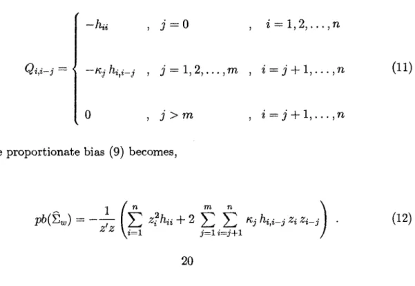
follows D.

4. BIAS OF THE HAC ESTIMATORS

In this Section one shows that the finite-sample performance of the Newey and

West estimator is related to the design of the matrix X. The importance of this

design is more general than the purposes of this Chapter and should be evaluated,

by using some diagnostic measure, in any applied econometric work. Such an

impor-tance can be explained briefly as follows [see Pollock (1979), Chapter 5). Due to the

fact that in the regression context the vector y does not belong to the space spanned

made in two main steps: first y is projected into

y

E M(X) by a projection matrix H, where fj =

H

y; the value of {3 is derived in the second step by minimising the distance between

y

and4 f)=

xp.

Considering the problem under the above explanation, the relation between estimated and true values, depends on the elements of the projection

matrix, as can be seen by the following expressions:

n

fli

= hiiYi+

L

hiiYi '

. #=i

n

ei

=

(1 -

hii)ci-

L

hijCj

#i

Knowing that hii is a measure of the distance of the point Xi from the bulk of the

points in X, one remote point leads the regression hyperplane to pass near this point5.

This fact can be responsible for some undesirable non-linearities in the data pattern

and therefore data points with leverage can worsen the finite-sample performance of

the model. 6.

As pointed by Huber (1973),

8fh/8yi

= hii and the inverse of hii can be thought as the equivalent number of observations that determine

Yi·

He also suggests points

with hii

>

0.2 to be classified as high leverage points. Others, like Belsley et al.

(1980) define as high leverage observations with corresponding diagonal element of

H greater than two times the mean of the hii1

S (note that

h

= (1/n)

Ei

hii = k/n). Good references in these topics are Huber (1981), Cook and Weiseberg (1982) and

Chatterjee and Hadi (1987).

To assess the effect of leverage points on the finite-sample performance of the

Newey and West estimator one requires some measure that allows us to confront it

under slight perturbations made to the design. To deal with this, one will nse the

4_{With this procedure one finds II= X(X'x)-}1_X'.

5_{When hii is high,}

_fii

_{is approximately equal to Yi and consequently the correspondent residual}

is approximately equal to zero.

proportionate bias that is no more than the bias scaled by the true value. Thus, for

any chosen combination,

w,

of the parameters in ~1,

w/3,

the proportionate bias of

---Var( w'

lJ)

=

Ew

is given by,

or,

--.

z'Qz

pb(~w) =

----;n ,

Z .l£Z (9)

where

z

= Zw is considered for simplifying purposes and

Q

=

E(fi)-

n.

Defining hi and Oi as the ith column of H and 0, respectively, the generic element of

Q

becomes,

' j =0 i=1,2, ... ,n

Qi,i-j = 1'\,j (ni,i-j -

h~ni-j-n~hi-j

+

hiD.hi-j)-ni,i-j ' j = 1, ... ,m ' i = j

+

1, ... ,n

(10)

,

j>m

,

i

= j

+

1, ...

,n

amount and the direction of this dependence. In a heteroskedastic model with non

autocorrelated errors Chesher and Jewitt (1987) found appropriate bounds, in the

finite-sample case, for the bias of the White's HCCM estimator and have shown a

straight relation between this bounds and the design of the X matrix. However, if the

errors are not independent their methodology7 does not seem to be possible because the matrix Q is not of a diagonal type, presenting a more complex structure.

There-fore, as an alternative, the bias of the Newey and West estimator and its relations with

the design of the X matrix will be studied via examples of three particular cases:

in-dependent, AR(l) and MA(l) errors. In each case, homoskedastic errors are assumed.

These examples allow us to draw a better idea of how important the design can be to

explain the bias and if this importance depends on a particular structure of the errors.

The main example considered in this Section, is the linear model (1) and the

MacKinnon and White (1985) data8, with 50 observations and three regressors,

X =

(XI

X2 X3J, where

X1

is a vector of ones and _{X 2} and _{X 3} are the rate of

growth of real U.S. disposable income and the U.S. treasury bill rate, respectively,

seasonally adjusted, for the period 1963-3 to 1974-4. The dependent variable is

de-termined by the linear relation (1)' given a particular

n

matrix.

4.1 Choice of the lag truncation

One of the problems related to the computation of the Newey and West estimate

is the derivation of the optimal value for the lag truncation parameter. White and

Domowitz (1984) and Andrews (1991) gave some insight to this problem9. Andrews

(1991) in the context of kernel HAC estimators has derived automatic bandwidth

7_{In particular the derivation of an algebraical expression for the eigenvalues, .A, solution to the}

characteristic polynomial

IQ

-

.AD! = 0.

8_{See table 3.}

9_{Recently Newey and West {1994) suggested a non-parametric method for automatically selecting}

estimators, where the value of the optimal bandwidth parameter is a function of

the number of observations and the structure of X'f [see Andrews(1991), pgs.

832-35, in particular his expressions (6.2) and (6.4) to (6.8)]. The structure of X'€ can

be assessed specifying k univariate approximate parametric models for { Xatet} for

a = 1, ... , k. The estimated parameters of these models are next used to compute the optimal m. However, in general, there is no a priori information about the best

approximated parametric model and this fact can be seen as an inconvenience of the

application of Andrews' method.

Another possible problem, not yet studied, is the performance of these

approxi-mate parametric models when the design of X has one or more leverage points and

therefore, its effects on the derivation of the optimal value of m. Suppose for example

that the sequences of observations { Xatft}

?=

_{1 ,} for each a = 1, ... , k , are generated by a zero-mean AR(1) process. If contamination is added to the observed value Xatfl,

l = 1, ... , n, one says that one isolated additive outlier occurs, in the terminology of Fox (1972). In this case the point (xa_{1_1}fi__{11 Xa1}f1) is an outlier in the response

vari-able and (xalfl, Xal+1il+1) a leverage point. As a consequence, the usual LS method

will yield biased parameter estimates, meaning that the resulting observations no

longer obey the AR(1) model. Finally, Andrews' procedure gives an optimal value

for m whichever the direction w has. As the following example suggests, this value

should depend on this direction, particularly when the data contains one or more

leverage points.

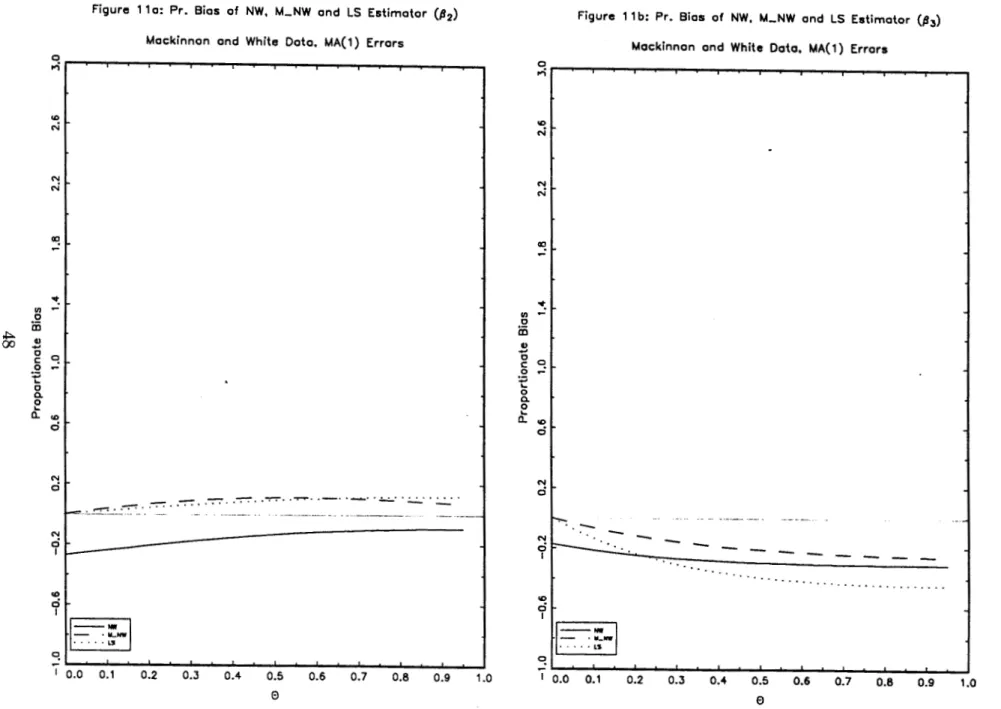
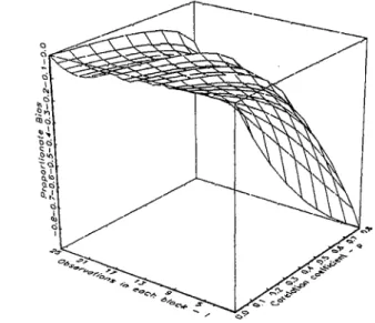
Using the Mackinnon and White data and the model (1) with AR(1) errors, figures

1a and lb show the proportionate bias of the Newey and West HAC estimator of

132

and (13, respectively, as a function of correlation coefficient and lag truncation.

Table10 1 shows the optimal value of the lag truncation associated with each value

1

°For each p this table gives the values of m in which the absolute value of the proportionate bias

of the correlation coe:fficient11. By optimal value, one means the value for which the

proportionate bias is minimum. As can be seen, the shape of the proportionate bias

and the optimal value of the lag tnmcation associated with {12 and f3a are very

differ-ent. This difference is due to the presence of a high leverage point in the Mackinnon

and White data (the 48th data point) in the direction of {3₂ [see Chesher and Austin

(1991), pag. 160]12. When measured by the diagonal elements of the hat matrix,

the correspondent value associated with the 48th data point is h48,48 = 0.39,

approxi-mately two times the limit value suggest by Huber and 6.5 times the mean of the hii 's.

Table 1-0ptimal value for the optimal lag truncation as a function of p

(AR(1) Errors, Mackinnon and White data)

0.0 0.1 0.2 0.3 0.4 0.5 0.6 0.7 0.8 0.9

0

0

0

1

0

2

0

0

1

3 4 5

2

6

5 10 16

8 12 13

The same conclusions can be drawn for the case with MA(1) errors. The difference

is only on the optimal value for the lag truncation that should be approximately equal

to one [see table13 2 and figures 2a and 2b].

West estimator of Var(,Bi), i = 1,2.

11 _{Note that what these pictures show are not simulated but e."~cact values.}

12

Deleting this point, the proportionate bias and the optimal lag truncation associated with 132

and

/33

are approximately equal.

13

Table 2-0ptimal value for the optimal lag truncation as a function of () and p

(MA(1) Errors, Mackinnon and White data)

p 0.00 0.10 0.192 0.275 0.345 0.400 0.441 0.470 0.488 0.497

() _{0.0 0.1 0.2 0.3 0.4 0.5 0.6 0.7 0.8 0.9}

m*(,B2)

0 0 0 0 0 0 0 0 0 0

m*(/33)

0 1 1 2 2 2 2 2 2 2

In the following a fixed lag truncation for different structures of the errors is

con-sidered. This simplification does not change the conclusions achieved for the relation

between bias and leverage.

4.2 Independent and Homoskedastic Errors

With independent errors the generic element of Q. in expression (10) simplifies to,

' j =0 i=1,2, ... ,n

0 ' j>m , i=j+1, ... ,n

and the proportionate bias (9) becomes,

However this expression does not give us a good guidance to the knowledge of how

large it can be. Following Chesher and Jewitt (1987), a better way is to bound the

above expression by using the following mathematical device,

z'Qz

sup-,-= max(.Ai) ,

z

z z

. f

z'Qz

. (, )

m - , -

=

m1n "'i ,

z

z z

(13)

where the .A/s are solutions of the characteristic equation, I

Q

-

)..J I= 0. Unfor-tunately the computation of the eigenvalues by I

Q

-

)..J I= 0 is not algebraically workable due to the fact that Q is a band matrix, with bandwidth equal to the lag

truncation.

Alternatively, if

z

is the eigenvector associated with the eigenvalue ).. it is well lrnown that

(Q-

)..J)

z

= 0. Therefore, for each i = 1:2, ... ,

n,

and Zi

=f.

0,

(qii- .A) Zi+

L

qij Zj = 0 '

#i

and the generic expression for the eigenvalues becomes,

or, by (11),

A= qii+

L

O'.ij qij '

#=i

A = -hii-

L

x;li-jl O'.ij hij '

j.p.

ii-Jism

with aij = Zj/Zi. Applying Gerschgorin's circle theorem (see for example Strang

(1980)), "every eigenvalue of Q lies in at least one of the circles Ci, i = 1, 2, ... , n,

where Ci has its centre at the diagonal entry qii and its mdi1ts equal to the ahsolute

sum along the rest of the row". Therefore, assuming from now on that "'li-il are the

weights defined by Newey and West, this theorem implies that

I

A

+

hii

I

s

L

Kli-il hij

I '

#i

li-,il~m

and the eigenvalues of

Q

lie in the ith circle, i.e., A is bounded by,

L

Kli-jl

I

hij

I

sA s -hii+ Hi

li-jj~m

L

Kli-jl

I

hij

I .

#i

li-jl ~m

(15)

(16)

To better evaluate this inequality, in particular the maximum and minimum value of

the right and left hand side, respectively, one will make use of the following lemma

[see for example, Cook and Weisberg (1982)),

Lemma 1: The hat matrix, H, has the properties:

1. if hii

=

1 then hij

=

0 for all j =/= i;

2. if hi·i

=

0 then hij

=

0 for all14 j;

4. if h7j = hii(l- hii) then

I

hij

I

is at its maximum value and hTk = 0 for all k =/= i, j.

Proof: Due to the fact that H is an idempotent matrix, hii can be written as

hii

=

Ej=

1 h~j = h;i

+

h;j

+

L~:f=i.i h;r and 1 and 2 follows immediately. To prove part

3 and 4 note that the above equality can be written as hii(1- hii)

=

hTi

+

E~:;t:i.j h;r

(see Cook and Weisberg (1982) and Chatterjee and Hadi (1988)]. D

Whichever the values of Kii-il and hij can be, it follows from lemma 1 that when

hii -+ 1, Ai -+ -1 and when hii -+ 0, Ai -+ 0. As a first conclusion, downward bias

.

equal to its minimum value is attainable, when hii = 1.

Part 3 and 4 of lemma 1 show a straight relation between hii and hij· Thus,

for a given value of hii the maximum of A depends only on the sum of the right

hand side of (16). Applying lemma 1 to this sum, its maximum value is attained at

I

hij

I=

h:/2

(1-

hii)112 and15

I

i -j

I=

1. Therefore, having in mind these results and expression (13) one has,

(17)

Considering the Newey and West estimator one has, K 1

=

mj(m

+

1). In particular, if m = 1, A is limited above by 0.0591, when hii = 0.053. The question that arises at this point is to know if this limit can be attained. A theoretical answer to this

ques-tion was not possible through this paper. However, from the examples considered,

some of which are presented below, there are reasons to believe that the maximum

eigenvalue of Q is not greater than zero.

Additionally, inequality (16) or (17) shows a straight relation between

proportion-ate bias and leverage. An illustration can be seen in the following example. Using

the Mackinnon and White data and the linear model (1) with N(O, 1) errors, one will

15_{Note that}

control the leverage associated with the 48th data point in the direction of {3_2• For

m

=

1 figure 3 shows the proportionate bias and the bounds for the proportionate

bias16 as a function of the leverage associated with the 48th data point. If the pro-portionate bias is sensitive to the leverage associated with the 48th data point then it

should change, as h48,4s changes. In fact when h48,48 increases, the proportionate bias

associated with (:J2 tends towards its minimum value. However such a dependence is

not straightforward. It depends also on the particular direction considered. In this

sense the Newey and West estimator is drastically downward biased if it is computed

in a direction for which there exists an observation with a high leverage.

In a second example, the relation between leverage points and the proportionate

bias is assessed by considering a simple model with one regressor,

{J i = 1

1 'todd

-1 i even

where fJ E ~. In this case the proportionate bias, for all w, becomes,

Forfixedn, when17 fJ---+ oo, h11(b) = (62 / (62 +n-1)) ---+.1 andpb(t)---+ -1. This

16_{With non-autocorrelated errors the proportionate bias is expressed by z'Qzf z' z. The supremum}

and infimum of this ratio over z are given by the maximum and minimum of the >.i 's values,

respectively, solutions of the characteristic equation

l

Q - >.I

l=

0.

17

In a regression problem with one regressor L~=l hii = 1. Therefore when hu-+ 1 , hii-+ 0 for

relation is pictured in figure 4 and as can be seen, the proportional bias is negative.

When

8

---+- 1,

hii(o)

---+- 1/n, the design becomes well balanced, where each point contributes equally to the regression line. In this case the proportionate bias depends

only on the value of the lag truncation with a maximum value of -1/n (when m

=

0)

and a minimum value that tends towards -1 as m approaches

n.

The value of the

proportionate bias is only explained by the autocorrelation structure of the residuals

that are never independent, even though when errors are independent.

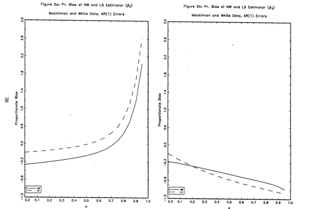
4.3 Non-independent and homoskedastic errors

In this subsection, model (1) and the Mackinnon and White data are considered in

two situations: AR(1) errors and MA(l) errors. In the case of AR(1) errors, figures

5a and 5b show the proportionate bias of the Newey and West and LS estimators

associated with

fj

2 and

'fia,

respectively, as a function of the correlation coefficient,

with m = 2 and p E [0, 0.9) in steps of 0.1. For the moment, three points should be kept in mind: 1) The LS variance estimator is not dominated by the Newey and West

estimator and for small values of pit performs better18_{; 2) the shape of the}

propor-tional bias associated with the variance estimators of

jj

2 and19

jj

3 are very different

and 3) the absolute value of the bias increases significantly when p approaches the

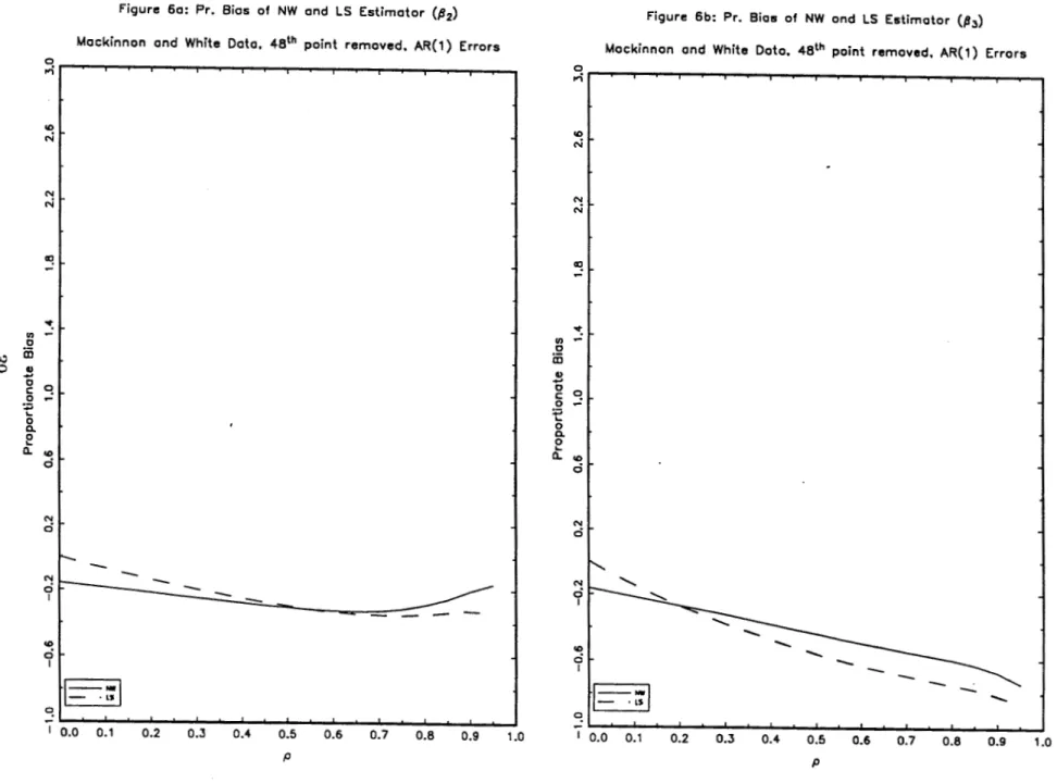
upper limit20• As seen above, this difference in the shape of the proportionate bias

is due to the presence of a leverage point in the direction of {32 • Therefore, if the

proportionate bias is sensitive to this kind of observations, then deleting this point

should have some effect on it. In fact the deletion of this point leads to a change in

the shape and, in general, a reduction (in absolute value) in the proportionate bias

associated to

/32

[see figs.6a and 6b).

18 _{A slight modification of the NW estimator with improved results for small values of p will be}

-

-presented in the next section.

19_{Selecting w}1 ₌

[0 1 OJ and w1 _{= [0 0 1 J respectively.}

20_{1t should be noted that part of thi'S increasing is due to the fact that the value of the lag}

Another interesting problem is the knowledge of the proportionate bias for all

pos-sible directions w E ~, considering expressions similar to

(13),

with the difference

that the denominator is now given by

z'Oz

.

Letting, for example Amax

=

max(Ai), the vectors

z*

that satisfy,

z'Qz

-,;:;- = Amax, Z ~£Z

are the eigenvectors associated with Amax, solutions to

(Q-

Amaxn)

z

= 0. To these vectors the proportionate bias (9) attains its maximum value. However because the

matrix X is fixed, expression

(13)

should be evaluated with care. The main reason is

that both Amax (Amin) and z depend on the design of X and therefore the supremum

(in:finum) over z should be calculated subject to the restriction of X fixed. Otherwise,

if X changes, resulting for example from the evaluation of expressions similar to

(13),

the eigenvalues no longer will be the same. In this sense and having in mind the

relation z* =

X(X' Xt

1w*, the direction for which the proportionate bias attends its maximum becomes equal to w* =

X'

z* (i.e., a linear combination of the rows of X, where the parameters of this combination are the elements of the eigenvector

associated with Amax)21_{• The proportionate bias and its bounds, viewed as function}

of p, are pictured in figure 7.

In order to eliminate some of the drawbacks associated with the evaluation of the

supremum and in:finum of (9), the effects of leverage points on the bounds of the

proportionate bias will be assessed by means of,

w'Aw

s u p - - = max(-\i) ,

w w'Bw

'nf w' Aw _ . ( , )

1 - B -rmn -"i ,

w w' w

21_{The same kind of reasoning could be made to min(>.i)·}

with A= (X'X)-1_X'QX(X'X)-1 _{and B = (X'X)-}1_X'rlX(X'X)-1

• The advantage

of this expression is that w does not depend on X and all the dynamic of this matrix

is incorporated in

A

and

B.

Therefore these bounds can be controlled in an

appro-priated manner by changing the design of the X matrix. As before these effects will

be assessed controlling the leverage associated with the 48th point. Figures 8 a), b)

and c) present these results form = 2 and p equal to 0.2, 0.5 and 0.8, respectively.

The first conclusion extracted from these pictures is that leverage points seem to

affect both the lower and upper bounds. However, the way in which each one of

these bounds is affected depends on the value of p. The second conclusion is that the

effect on the lower bound is more important for small values of p. When p = 0.8, for example, this bound does not seem to be influenced for h48,48

<

0.9,

approxi-mately. However, while the lower bmmd remains constant the upper bound change

with h48,48· The third conclusion is that _{h 48,48} does not affect both, lower and upper

bounds altogether (when one changes the other remains constant). Finally there is

a possibility of upward bias for a moderate leverage associated with a high value

of p. This is the case of the proportionate bias of the Newey and West estimator of

Cov({J':l.),

showed in figure Sc. However, this possibility should be evaluated with care, due to the non-monotonicity of the upper bound, relatively to h48,4s. When p = 0.8

the maximum bias is attainable for h_48,48 approximately equal to 0.5.

Figures 9 a), b) and c) present the same results for the case of MA(l) errors, with

m = 1 and 0 equal to 0.2, 0.5 and 0.8, respectively. The only difference to the above

case is that the bmmds appear to be less pronmmced and more robusts to leverage,

4.4 Modified Newey and West Estimator

In this Section a slight modification of the Newey and West estimator is presented.

This modification is based on an additive bias correction for the particular case of

in-dependent and homoskedastic errors. Multiplicative corrections are also possible but

only for the diagonal entries of X'ftX. With independent errors the autocorrelation

structure of the residuals can only be eliminated by an additive term.

It is well known that even when errors are homoskedastir. and independent,

con-ventional least-squares residuals never have these properties. In particular

E(en

=

o-2

(1-

hii) and

E(fifj)

= -a2_{hij· Therefore instead of X'OX}

given in expression (7)

the following estimator of X'DX is suggested,

n m n

X'O* X=

L

(~

+

&

2

hii)x~xi+

L L

Kj (iifi-j

+

&

2

hi,i-i)(x~Xi-j

+

x~_jxi)

,

(19)

i=l j=li=j+l

where &2

=

L:f=

₁

qj(n- k).

With homoskedastic and independent errors,

E(fj:U)

=

~w = a2

(X'X)-

1_{. Moreover this estimator (as well the Newey and West estimator)}

is asymptotir.ally unbiased sinr.e hii - t 0 as n - t oo.

To prove the positive semi-definiteness of the modified Newey and West estimator,

consider (19) expressed in matrix form as,

X'O* X =X' OX+ &2 X'QX

with the elements of

Q

defined as the symmetric of (11).

Theorem 2: The modified Newey and West estimator is positive semi-definite.

Proof. For a proof it is sufficient to apply theorem 1 of Newey and West (1987) to

the second term of the right hand side of the above expression. By doing that X1

is positive semi-definite and the result of the theorem follows.D

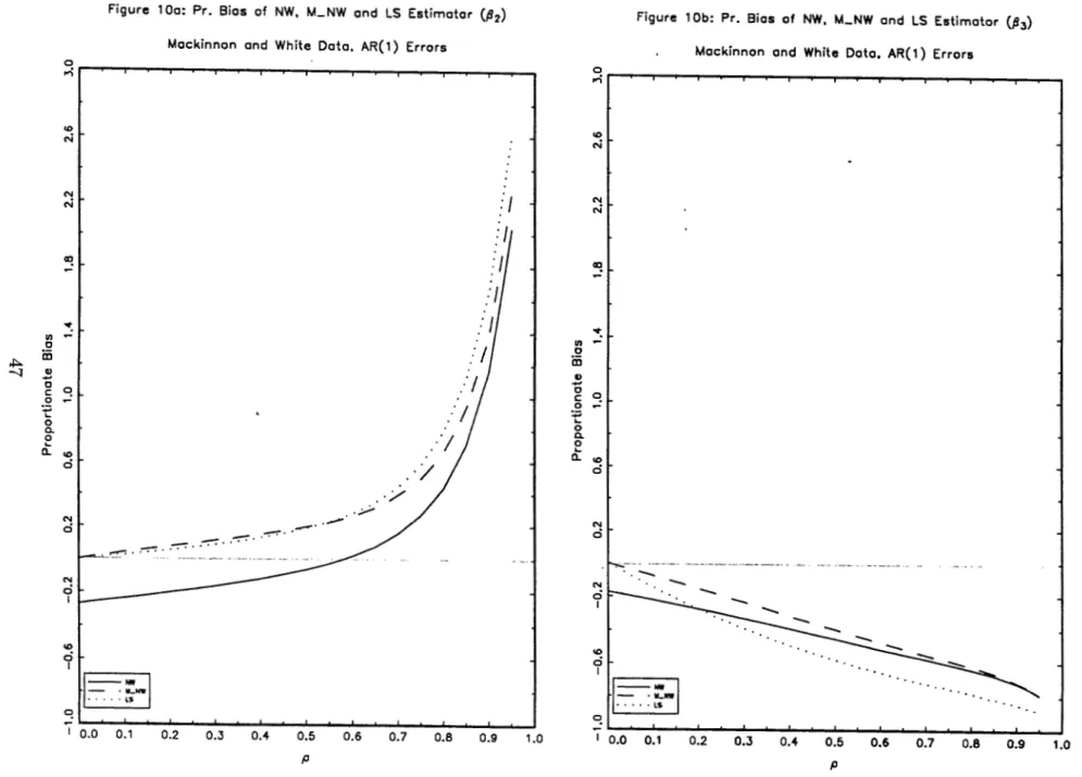
A bias comparison between the modified Newey and West, Newey and West and

LS estimators are pictured in figure 10 and 11, using the Mackinnon and White data,

for AR(1) and MA(1) errors, respectively. As it can be seen by these pictures, the

proportionate bias of the modified Newey and West Estimator associated with

fj

₃ performs better than the other estimators for the values of p and (} in the interval

[0, 0.9]. However,· this conclusion is not clear if the proportionate bias is computed

in a direction of a covariate with an important leverage as can be seen from pictures

lOa and 11a.

5. THE FINITE-SAMPLE DISTRIBUTIONS OF

HETEROSKEDASTICITY AND AUTOCORRELATION ROBUST

WALD STATISTIC

The subject of this Section is a natural extension of the results presented above. In

the econometric framework, it is well known that hypothesis tests require a consistent

estimator of scale. However when this estimator presents an important bias, as in

the case of the Newey and West estimator and the sample size is not large enough,

it is important to know how this fact can affect inferences based on the asymptotic

distribution. For this reason this Section is concerned with the performance of the

first order asymptotic normal approximation to the finite-sample distribution of the

Wald test statistic, when the variance estimator of

fJ

is HAC type.

Mackinnon and White (1985) provided Monte Carlo estimates of the exact sizes of

nominal5% and 1% two-sided tests under the null hypothesis, using different HCCM

on the regression design. Thus, the conclusions derived from this procedure can be

very misleading, as shown by Chesher and Austin (1991). These authors derived the

exact finite-sample distributions of heteroskedasticity robust Wald statistics of scalar

linear hypotheses in the normal linear model. Moreover they showed a

straightfor-ward relation between the regression design and the quality of these approximations.

In this Section their methodology is extended to the case in which the variance

estimator of

fj

is HAC type. In particular, the quality of the asymptotic normal approximation to the finite sample distribution of the test is assessed in the case

of independent and AR(1) errors for different configurations of the design of the X

matrix.

C~msidering the linear model presented in Section 2, the Wald test statistic for the

hypothesis Ho: w' (3

=

Wo is given by,

w'/i-

Wo

t=

~

(w':Ew)l/2

(20)

In the following, consider that the null hypothesis is true. Thus, if X obey to some

suitable conditions as the Grenander conditions [see for example Judge et al. (1985)),

t

converges in law to the standard normal distribution. Deviations of the finite sample

distribution oft from its asymptotic distribution will be the measure of the quality

of this test statistic.

Assuming

w'f3

=

w

0 , the numerator of

t

2 can be written as,

where

A=

n

1₁2

zz'n

1₁2 _and

_z

_{was defined in Section 4. For the denominator one has}

as well,

w''Ew =

z'Oz

= u' Bu

where B =

2:i=l

zin112mimin112zi

+

2

2:j=12:r=j+l

Ki-jZjn112mjmin112zi. Both,

nu-merator and denominator of t2 , are quadratic. forms in normal variables and the

distribution of t2 can be calculated using the procedure given by Imhof (1961). Due

to the fact that

A

and Bare symmetric matrices, it follows that

A-

c2

B

is also sym-metric, being possible the spectral decomposition, A-c2 B = LD.L', with L' L

=

I. As a consequence, when w'

p

= w0 one has,

n

P(t2

<

c2) = P[u'(A-c2 B)u

<

0]

=

P[2:

rJoi

<

0] ,

(21) i=l

where ri = u'li "" N(O, 1), li is the ith column of L and 8i the eigenvalue associated with li. Finally, the probability in the left hand side of (21) is computed by the

following,

n 1 1 /00 sinO(v)

P(t2

<

c2) = P[I:r;oi

<

0]

= -

+-

( )

dv,

i=l 2 7r o vp v

(22)

where,

n

B(v) = 0.5

L

arctan(8iv)

i=l

n

p(v)

=IT

(1

+

8lv2)1/4

Because the null distribution of t is symmetric around zero, its determination from

the distribution of t2 is possible, having in mind the relation,

P(t2

<

c

2) = 2P(t

<

c)-

1

for any scalar c

>

0.

Considering the linear model (1) and the Mackinnon and White data, Figures22 12 to 15 show upper halves of the exact finite-sample distribution functions of the

Wald tests, using the Newey and West estimator with a fixed lag tnmcation, when

the errors are independent and AR(1). In this case p = 0.2, p = 0.5 and p = 0.8, respectively. In each of these Figures one considers the hypotheses

/32

= 0 on the left and

/33

= 0 on the right.

From these pictures, one condudes that the exact distribution is less well

approx-imated by the standard normal distribution as the correlation coefficient increases.

However the quality of this approximation seems to depend on the particular

hy-potheses considered. The distribution function of the Wald test moves far to the

right of the standard normal in the

/33

= 0 case and to the left in the

/32

= 0 case. As seen before the main reason for this difference in the shape of the exact distributions

is due to the presence of the 48th leverage point. Deleting this point [figure not

pre-sented] both distributions present the same shape.

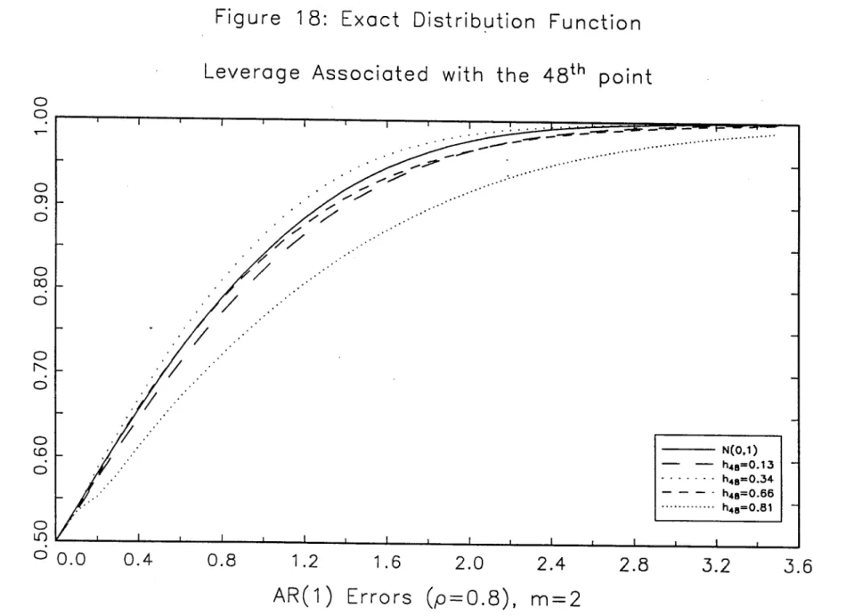
A more accurate way to evaluate the dependence of the exact distribution on the

regression design is by controlling the leverage associated with one particular

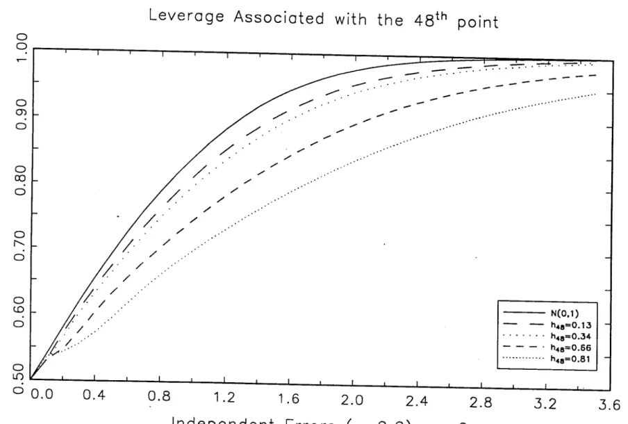
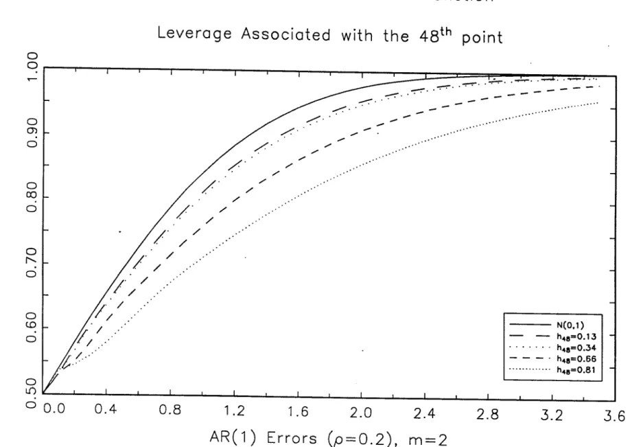
obser-vation, following the same methodology described in Section 3. Figures 16 to 18 show

upper halves of the exact distribution for different values of the autocorrelation of the

errors. In each of these pictures the 48th point is equal to (1, 6), with 8 E ~replaced

by some appropriated value, corresponding to h48,48 equal to 0.13, 0.34, 0.56 and

0.81. With independent errors [see figure 16), as the leverage associated with the 48th

point increases, the exact distribution moves far to the right of the standard normal,

presenting long tails. However, with

AR(l)

errors, particularly for high values of p,

this effect should be evaluated with care, due to the non monotonicity between h48,₄₈

and the shape of the exact distribution. For low and high values of h48,48 the exact

distribution is to the right of the standard normal. For moderate values of h48,48 the

exact distribution moves to the left of the standard normal, presenting a greater peak.

A possible reason for this behaviour can be due to the upward bias of the Newey and

r , ... ,<: ...

..,

<Q. ... .... 0

-

0 E :;:; Ill

.,

!t z

-

0 _.... Ill Ill 0

0 ...

...

iii w

.,

...

-

~

0 ...

c 0::

0 <

:;:; _... 0 Q, 0

a:

.i:i

.,

...

::J 01 iL ... N <Q. ...

...

0 0 .~

-Ill I ) 3: z

-

0 ... 0)

Ill 0

.~ L. ... m w

I ) ...

-

0 ...

c 0::

.~ <

-

... 0 Q, 0 ... Q. 0 I ) ... ::J 01 iL

!i"t o·t !i·o o·o

""'"' _CQ.

..,

... .... 0

-

0 .~

-

Ill

.,

3:

z

.... ₀ Ill ...

Ill 0

• !:! .... ....

ID w

II ""'"'

-

....

D ... 1: < 0 :E

:;:; _.... 0 a. 0 .... 0.. ..i:i N

.,

.... ;:, .!? LL. ...

..

CQ. ... L 0 0 .~

-

Ill

.,

3:

z

0 Ill

L

Ill 0 L

.!:! L

ID w

...

I )

....

-

D ...

1: <

.!:! ::e

-

L 0 a. 0 .... 0.. 0 N

.,

L ;:, 01 i;:

1 ·o o·o- ,·o- ;ro- £"0-

0

\.._

0

-+-' OJ

0 ₀

E

I

-+---'

(()

L..U

I

CX)

-+---' 0

(()

I

(})

s

I

r-...

v

₀

c

I

0

>--, ₀

_I

(})

L() <..0

3 _II

I

0

(})

z

z

I

CXJ

4---~

0

---

L() .

II

_I

0 CXJ

<t-(()

E

..c

0

·-

_I

m

~

0 _~

(}) _II

0

-+-'

0 Q

c

0

I

-+---'

:

I

n

\.._

0 0

Q_

:

I

0

\.._

Q_

:

I

_N

0

n

_:I

X

Nn 0

(}) .<::: .0 .0 _E

\.._ EO... D...,<

:::::; ,<

..---OJ 0

·

-LL

0 0

0. l

_~ro

g·o

-v·o z·o

z·o-

g·o-

;_ 0 -+-' 0

E

-+-' (f)

w

-+-' (f) Cl)

5

u

c

0

>-Cl)

s

Cl)

z

'+-0 (f) 0 ·

-m

Cl) -+-' 0

c

0 -+-' L 0 Q_ 0 L Q_ ~ Cl) ;_ :::J CJl LL 0 L() II

z

~ II

E

~ 0 II Q

+

·-_{,...---..._} ~ '-.,___/ II X G() II X

..

;_ 0 (f) (/) Cl) ;_ CJl Cl) ;_ (])

c

0 0

I

/

,/ CJ'>