Bias and size effects of price-comparison search engines: theory and experimental evidence

Bias and Size Effects of Price-Comparison Search

Engines: Theory and Experimental Evidence

⋆

AURORA GARCÍA-GALLEGO

†

NIKOLAOS GEORGANTZÍS

‡

PEDRO PEREIRA

§

JOSÉ C. PERNÍAS-CERRILLO

¶

1st November 2005

We analyze the impact on consumer prices of the size and bias of price comparison search engines. In the context of a model related to Burdett and Judd (1983) and Varian (1980), we develop and test experimentally several theoretical predictions. The experimental results confirm the model’s predictions regarding the impact of the number of firms, and the type of bias of the search engine, but reject the model’s predictions regarding changes in the size of the index. The explanatory power of an econometric model for the price distributions is significantly improved when variables accounting for risk attitudes are introduced.

Keywords: Search engines, incomplete information, biased information, price levels, experiments.

JEL Codes: C91, D43, D83, L13.

Corresponding author: Prof. Nikolaos Georgantzís:Dep. Economia, Universitat Jaume I, Av. Vi-cent Sos Baynat, 12071 Castellón (Spain); e-mail: georgant@eco.uji.es; phone: 34-964728588.

⋆

The authors gratefully acknowledge financial support by the NET Institute, the Spanish Ministry of Science and Technol-ogy (BEC2002-04380-CO2-02), and the Generalitat Valenciana (GREC-GRUPOS04/13). This paper benefited from helpful comments by S. Hoernig, and professors H. Raff and J. Bröcker during the Erich Schneider seminar at Kiel Universität, T. Ca-son and J. Brandts at the IMEBE meeting in Córdoba, seminar participants at the Universities of Salamanca, Murcia, Paris II, Siena, Complutense de Madrid, and other participants at the SPIE (Lisbon), The Economics of Two Sided Markets (Toulouse), EARIE (Berlin), ASSET (Barcelona), and XX Jornadas de Economía Industrial (Granada) meetings.

†_{LEE/LINEEX and Economics Department, Universitat Jaume I, Castellón (Spain); e-mail: mgarcia@eco.uji.es; phone:} 34-964728604.

‡_{LEE/LINEEX and Economics Department, Universitat Jaume I, Castellón (Spain); e-mail: georgant@eco.uji.es; phone:} 34-964728588.

§_{Autoridade da Concorrência, R. Laura Alves, n}o_{4, 7}o_{, 1050-138 Lisboa (Portugal); e-mail: jppereira@oninetspeed.pt;} phone: 21-7802498; fax: 21-7802471.

Bias and Size Effects of Price-Comparison Search

Engines: Theory and Experimental Evidence

We analyze the impact on consumer prices of the size and bias of price comparison search engines. In the context of a model related to Burdett and Judd (1983) and Varian (1980), we develop and test experimentally several theoretical predictions. The experimental results confirm the model’s predictions regarding the impact of the number of firms, and the type of bias of the search engine, but reject the model’s predictions regarding changes in the size of the index. The explanatory power of an econometric model for the price distributions is significantly improved when variables accounting for risk attitudes are introduced.

Keywords: Search engines, incomplete information, biased information, price levels, experiments.

1. INTRODUCTION

1.1. Preliminary Thoughts

From the consumers’ perspective, one of the most promising aspects of e-commerce was that it would reduce search costs. With search engines, consumers could easily observe and compare the prices of a large number of vendors, and identify bargains. The consumers’ enhanced ability of comparing prices would discipline vendors, and put downward pressure on prices.1

Price Comparison Search Engines, also known as shopping agents or shopping robots, are a class of search

engines, which access and read Internet pages, store the results, and return lists of pages, which match keywords in a query. They consist of three parts: (i) a crawler, (ii) an index, and (iii) the relevance algorithm. TheCrawler,

or spider, is a program that automatically accesses Internet pages, reads them, stores the data, and then follows links to other pages. TheIndex, or catalog, is a database that contains the information the crawler finds. The Relevance Algorithmis a program that looks in the index for matches to keywords, and ranks them by relevance,

which is determined through criteria such as link analysis, or, click-through measurements. This description refers to crawler-based systems, such as Google or AltaVista. There are alsoDirectories, like Yahoo was initially, in

which lists are compiled manually. Most systems are hybrid.

Presumably, the larger the number of vendors whose price a search engine lists on its site, and that thereby consumers can easily compare, the more competitive the market becomes. However, there are several technical reasons for search engines to cover only a small subset of the Internet, and to collect and report information biased in favor of certain vendors. This perspective is discussed in Pereira (2004) and documented by several studies (Bradlow and Schmittlein, 1999; Lawrence and Giles, 1998, 1999).

The technology-induced tendency, for search engines to have incomplete and biased coverage, is reinforced by economic reasons. Search engines are profit-seeking institutions, which draw their income from vendors, either in the form of placement fees, sales commissions, or advertising (Pereira, 2004).

In this paper we examine, theoretically and experimentally, the impact on consumer prices on electronic mar-kets, of price comparison search engines covering only a small subset of the Internet, and collecting and reporting information being biased in favor of certain vendors.

1.2. Overview of the Paper

We develop a partial equilibrium search model, related to Burdett and Judd (1983) and Varian (1980), to discuss the implications of price comparison search engines providing consumers with incomplete and biased information. There is: (i) one price comparison search engine, (ii) a finite number of identical vendors, and (iii) a large number of consumers of two types. Shoppers use the price comparison search engine, and buy at the lowest price listed by the search engine. Non-shoppers buy from a vendor chosen at random. Vendors choose prices. In equilibrium, vendors randomize between charging a higher price and selling only to non-shoppers, and charging a lower price to try to sell also to shoppers.

In the benchmark case, the search engine has complete coverage, i.e., lists the prices of all vendors present in the market. We also analyze two other cases. First, the case in which the price comparison search engine has incomplete coverage, and is unbiased with respect to vendors. This case can be thought of as portraying the situation where the search engine is a crawler-based system, which has no placement deals with any particular vendor. Second, we analyze the case in which the price comparison search engine has incomplete coverage, and is biased in favor of certain vendors. This case can be thought of as portraying the situation where the search engine is either a crawler-based system or a directory, which has placement deals with certain vendors. The search engines’ decisions of how many vendors to index, or the vendors’ decisions of whether to become indexed, are obviously of interest. Pereira (2004) analyzes these questions. In this paper we take these decisions as given, and focus on the implications for the pricing behavior of vendors.

The theoretical analysis makes several predictions regarding the impact of: (i) the number of vendors, (ii) the size of the search engine, and (iii) the type of bias of the search engine. In addition, the model also draws

attention to four general counterintuitive effects. First, there is a conflict of interests between types of consumers, i.e., between shoppers and non-shoppers. This makes it hard to evaluate the welfare impact of these effects. Second, more information, measured by a wider Internet coverage by the price comparison search engine, is not necessarily desirable. It benefits some consumers, but harms others. Third, unbiased information about vendors is not necessarily desirable either, and for the same reason. Fourth, the effects of entry in these markets are complex, and depend on the way entry occurs.

We tested the predictions of the theoretical analysis, in a laboratory experiment designed to evaluate the model’s testable hypotheses. This included a lottery-choice task, intended to capture two different aspects of risk attitudes: (i) the subjects’ degree of risk aversion, and (ii) whether subjects accepted more risk in exchange for a higher return to risk.

The experimental results confirm the model’s predictions regarding the impact of the number of firms, and the type of bias of the search engine, but reject the model’s predictions regarding changes in the size of the index. The analysis of the data indicated several additional data patterns, such as, that prices are lower under biased incomplete coverage than under unbiased incomplete coverage.

We also developed an econometric model of the empirical price distributions. This lead us to a very interest-ing empirical findinterest-ing concerninterest-ing risk attitudes. Introducinterest-ing variables that account for the subjects’ risk attitudes improved significantly the explanatory power of the econometric model. The implication of this finding for future research is clear. If behavioral factors are systematically important in these markets, then they should be incorpo-rated explicitly in the modeling assumptions. Otherwise models may generate predictions that contrast with the empirical evidence.

1.3. Literature Review

The basic search models relevant for our research were developed in the early 1980s by Varian (1980), Rosenthal (1980), and Burdett and Judd (1983). Varian (1980) developed a model where firms are identical and there are two types of consumers. Shoppers, can observe costlessly all prices, while non-shoppers, observe only one price, perhaps because they have a prohibitive search cost. Firms randomize between charging low prices to try to sell to shoppers, and charging high prices to sell only to their share of non-shoppers. Stahl (1989) endogeneized the non-shoppers reservation price through sequential search, and performed several comparative statics exercises. He showed that for this class of models, the equilibrium price distribution ranges between the monopoly and the competitive levels, as the fraction of shoppers varies between 0 to 1.

Recently, the use of the Internet and the existence of price-comparison search engines, renewed the interest in the search literature. Baye and Morgan (2001) developed a model where firms can sell on their local market, or sell beyond their local market through the Internet. Similarly, non-shoppers are consumers buying locally, whereas shoppers are consumers buying over the Internet. The price equilibrium involves mixed strategies. Iyer and Pazgal (2000) developed another model of electronic commerce where firms play mixed strategies, and tested it empirically. Brynjolfsson and Smith (2000) also confirmed empirically the prediction of persistent price dispersion in Internet markets, even in the presence of homogeneous products.

2. THE MODEL

2.1. The Setting

Consider an electronic market for a homogeneous search good that opens for 1 period. There are: (i) 1 price comparison search engine, (ii) n≥3 vendors, which we index through subscript j=1, . . . ,n, and (iii) many

consumers.

2.2. Price-Comparison Search Engine

The Price-Comparison Search Engine, in response to a query for the product, lists the addresses of the firms

contained in its database, i.e., in itsIndex, and the prices they charge. The search engine may be of one of the

following types:

(i). Complete Coverage: Denote byk, the number of vendors the price-comparison search engine indexes. We

will refer tokas theSize of the Index. The search engine hasComplete Coverageif it indexes all vendors

present in the market:k=n.

(ii). Unbiased Incomplete Coverage: The search engine hasIncomplete Coverageif it does not index all vendors:

1<k<n. In addition, the search engine has anUnbiased Sampleif it indexes each of thenvendors with

the same probability: n−1

k−1

/ n_k=k/n. When the search engine has incomplete coverage and an unbiased

sample, we say that it hasUnbiased Incomplete Coverage.

(iii). Biased Incomplete Coverage: A search engine with incomplete coverage has aBiased Sampleif it indexes

vendors j=1, . . . ,k, and does not index vendors j=k+1, . . . ,n. When the search engine has incomplete

coverage and a biased sample, we say that it hasBiased Incomplete Coverage. For this parametrization,

knowing the probability with which vendors are indexed, implies knowing the identity of the indexed ven-dors.2

Denote byτthe type of the search engine, and let ‘c’, meanComplete Coverage, ‘u’ meanUnbiased Incom-plete Coverage, and ‘b’ meanBiased Incomplete Coverage, i.e.,τbelongs to{c,u,b}. We will use superscripts ‘c’, ‘u’, ‘b’, to denote variables or values associated with the cases where the search engine has that type.

2.3. Consumers

There is a unit measure continuum of risk neutral consumers. Each consumer has a unit demand, and a reservation price of 1. There are 2 types of consumers, differing only with respect to whether they use the price-comparison search engine.Non-Shoppers, a proportionλin(0,1)of the consumer population, do not use the price-comparison search engine, perhaps because they are unaware of its existence, or perhaps because of the high opportunity cost of their time.3_{The other consumers,Shoppers, use the price-comparison search engine.}

Consumers do not know the prices charged by individual vendors. Shoppers use the price-comparison search engine to learn the prices of vendors. If the lowest price sampled by the price-comparison search engine is no higher than 1, shoppers accept the offer and buy; in case of a tie they distribute themselves randomly among vendors; otherwise they reject the offer and exit the market. Non-shoppers distribute themselves evenly across

2. There are alternative ways of introducing sample biasedness, for which knowing the probability with which vendors are indexed does not imply knowing the identity of the indexed vendors. For example, all vendors can be indexed with a non-degenerate probability, which is higher for some vendors than for others. The advantage of our parametrization is that it yields a closed form solution.

vendors, i.e., each vendor has a share of non-shoppers of 1/n. If offered a price no higher than 1, non-shoppers

accept the offer and buy; otherwise they reject the offer and exit the market.

2.4. Vendors

Vendors are identical and risk neutral. Marginal costs are constant and equal to zero. Vendors know the functioning rules of the search engine. In particular, underUnbiased Incomplete Coverage, vendors know the probability with

which they are indexed, but do not observe the identity of the indexed vendors, before choosing prices. Under

Biased Incomplete Coverage, vendors know the identity of the indexed vendors before choosing prices. In the

cases of Complete CoverageandUnbiased Incomplete Coverage, vendors are identical. In the case of Biased Incomplete Coverage, vendors are asymmetric. Denote byΠ_j(p), the expected profit of vendor jwhen it charges

priceponR+₀. A vendor’sstrategyis a cumulative distribution function over prices,Fj(·). Denote the lowest and

highest prices on its support by

¯pjand ¯pj.

4_{A vendor’spayoff is its expected profit.}

2.5. Equilibrium

ANash equilibriumis an-tuple of cumulative distribution functions over prices,{F1(·), . . . ,Fn(·)}, such that for

someΠ⋆_jon_R+₀, and j=1, . . . ,n: (i)Πj(p) =Π⋆j, for allpon the support ofFj(·), and (ii)Πj(p)≤Π⋆j, for allp.

When vendors are identical we focus on symmetric equilibria, in which case:Fj(·) =F(·),

¯

pj=

¯

p, ¯pj=p¯and

Π⋆_j=Π⋆, for all j.

3. CHARACTERIZATION OF EQUILIBRIUM

Denote byφτ

j the probability of firm jbeing indexed, given that the search engine is of typeτ:

φτ_j =   

 

k/n ifτ=c,u

1 ifτ=band j=1, . . . ,k

0 ifτ=band j=k+1, . . . ,n.

Denote by ˆp−jthe minimum price charged by any indexed vendor other than vendor j, and denote by ˆm−jthe

number of indexed vendors that charge ˆp₋j. The profit function of vendor jwhen it charges pricepjis:

πj(pj;τ) =

                     pj λ

n+ (1−λ)φ τ

j

ifpj<pˆ−j≤1

pj

λ

n+

1−λ ˆ

m−j

φτj

ifpj=pˆ−j≤1

pj

λ

n if ˆp−j<pj≤1

0 if 1<pj.

Ignoring ties,5_{the expected profit of a vendor that chargesp≤1 is:}6

Π_j(p) =pλ

n +p(1−λ)φ τ

j[1−F(p)]k

−1_{. (1)}

Denote bylτ_j the lowest price vendor jis willing to charge to sell to both types of consumers when the search

engine has typeτ, i.e.,lτ_j[λ/n+ (1−λ)φτ_j]−λ/n≡0. The next Lemma states some auxiliary results.

4. As it is well known this game has no equilibrium in pure strategies (Varian, 1980). 5. Lemma 1(ii) shows thatF_jτ(·)is continuous.

6. A vendor jthat charges a price p≤1 sells to shoppers: (i) if it belongs to the set of vendors indexed by price-comparison search engine, which occurs with probabilityφτ_j , and (ii) if it has the lowest price among the indexed vendors, which occurs with probability[1−F(p)]k−1. Thus, the expected share of shoppers of a vendor that charges price p≤1 is:

Lemma 1. For all j:(i)lτ_j ≤

¯pj≤p¯j≤1;(ii)F

τ

j is continuous on[lτj,1];(iii) ¯pj=1;(iv)Π⋆j=λ/n;(v)

¯

pj=lτj;(vi)Fjτhas a connected support.

From Lemma 1(iv), in equilibrium:

pλ

n +p(1−λ)φ τ

j[1−Fjτ(p)]k−1=

λ

n. (2)

Denote byδ(p), the degenerate distribution with unit mass on p.7 The next proposition characterizes the

equilibrium for the model.8

Proposition 1. (i)forτ=c,u and j=1, . . . ,n, and forτ=b and j=1, . . . ,k:

F_jτ(p;n,k) =             

0 ⇐p<lτ_j

1− "

1

nφτ_j !

λ 1−λ

1−p p

#k−11

⇐lτ_j ≤p<1

1 ⇐1≤p,

with

lτ_j(n) = λ λ+ (1−λ)nφτ

j

;

(ii)forτ=b and j=k+1, . . . ,n, Fb

j(p;n,k) =δ(1).

UnderBiased Incomplete Coverage, vendors j=k+1, . . . ,n, are not indexed for sure, and therefore have

no access to shoppers. Since these vendors can only sell to non-shoppers, which are captive consumers, they charge the reservation price. Vendors j=1, . . . ,k, underBiased Incomplete Coverage, and all vendors in the cases Complete CoverageandUnbiased Incomplete Coverage, are indexed with positive probability. Hence, they face

the trade-off of charging a high price and selling only to non-shoppers, or charging a low price to try to sell also to shoppers, which leads them to randomize over prices.

4. ANALYSIS

In this section, we analyze the model for the 3 types of search engine.

4.1. Complete Coverage

In the case ofComplete Coveragethe model is similar to Varian (1980).9

Rewrite (2) as:

p(1−λ)[1−Fc(p)]n−1

| {z }

Marginal Benefit

= λ

n(1−p). | {z } Opportunity Cost

(3)

If a vendor charges a price plower than the consumers’ reservation price, it has the lowest price in the market

with probability[1−Fc_(p)]n−1_{, sells to(1−λ)shoppers, and earns an additional expected profit ofp(1−λ)[1−} Fc(p)]n−1_{: theVolume of Sales effect. However, it loses(1−p)per non-shopper, and a total of(1−p)λ/n: the} per Consumer Profit effect. The volume of sales effect is themarginal benefitof charging a price lower than the

consumers’ reservation price, and the per consumer profit effect is themarginal cost.

Denote byε, the expected price, i.e., the expected price paid by non-shoppers. And denote byµ, the expected minimum price, i.e., the expected price paid by shoppers.

7. Functionδ(·)is the Dirac delta function.

8. The equilibrium described in Proposition 1 is the unique symmetric equilibrium. Baye et al. (1992, Theorem 1, p. 496) showed that there is also a continuum of asymmetric equilibria, where at least 2 firms randomize over[l,1], with each other firmirandomizing over[l,xi),xi<1, and having a mass point at 1 equal to[1−Fi(xi)].

The next Remark collects two useful observations.

Remark 1. (i)λ εc_{+ (1−λ)µ}c_=λ;(ii)µc_<εc_.

The first part of Remark 1 says that the average price paid in the market,λ εc_+(1−λ)µc_{, equals the proportion}

of non-shoppers,λ.10 _{This has two implications. First, only shifts in the proportion of non-shoppers change the}

average price paid in the market. Second, shifts in any other parameter, such as the number of vendors,n, induce

the expected prices paid by shoppers and non-shoppers to move in opposite directions. A conflict of interests between types of consumers is a recurring theme of this paper.

The second part of Remark 1, says that the expected price paid by shoppers,µc_=lc₊R1

lc(1−Fc)nd p, is lower than the expected price paid by non-shoppers,εc_=lc₊R1

lc(1−Fc)d p. The price-comparison search engine allows shoppers to compare the prices of all vendors in its index, and choose the cheapest vendor. This induces competition among vendors and puts downward pressure on prices, which benefits consumers using search engines.

4.2. Unbiased Incomplete Coverage

In this subsection, we analyze the case ofUnbiased Incomplete Coverage, and compare it with the case of Com-plete Coverage. We show thatUnbiased Incomplete Coveragecompared withComplete Coverage, increases the

expected price paid by shoppers, and decreases the expected price paid by non-shoppers.

The price distribution for the case in which the market consists ofnvendors, and the price-comparison search

engine has an unbiased index of sizek≤n, is identical to the price distribution for the case in which the

price-comparison search engine has Complete Coverage, k=n, and the market consists of k vendors: Fu_{(·;n,k) =}

Fc(·;k). For further reference, we present this observation in the next corollary.

Corollary 1. Fu(·;n,k) =Fc(·;k).

The next proposition analyzes the impact of changes in the size of the index,k, and the number of vendors,n.

Proposition 2. (i)lu(k)<lu(k−1);(ii)µu_(n,k)<µu_{(n,k−1)andε}u_(n,k)>εu_{(n,k−1);(iii)F}u_{(·;n,k) =}

Fu(·;n+1,k).

Rewrite (2) as:

p(1−λ)

k n

[1−Fu(p)]k−1=λ

n(1−p). (4)

From (4), an unbiased decrease in the size of the index has two impacts. First, for indexed vendors, the decrease in the size of the index reduces the number of rivals with which a vendor has to compete to sell to shoppers from

k−1 tok−2. This increases the probability that an indexed vendor will have the lowest price,(1−Fu₎k−1_{, which}

increases theVolume of Sales effect. The first impact leads vendors to shift probability mass from higher to lower

prices. As a consequence, the price distribution shifts to the left (Figure 1). Second, the decrease in the size of the index reduces the probability that a given vendor is indexed fromk/nto(k−1)/n, which reduces theVolume of Sales effect. The second impact leads vendors to raise the lower bound of the support, and to shift probability

mass from lower to higher prices. As a consequence, the price distribution rotates (Figure 1). The total impact of an unbiased decrease in the size of the index is to cause the price distribution to rotate counter clock-wise.11

The increase in the lower bound of the support,lu(k)<lu(k−1), raises the expected price paid by shoppers, µu_(n,k)<µu_{(n,k−1). However, from Remark 1(i), the average price paid in the market remains constant and}

equal toλ. This implies that the expected price by non-shoppers decreases,εu_(n,k)>εu_(n,k−1).12 _{Recall that}

vendors now charge lower prices with a higher probability. Shoppers and non-shoppers have conflicting interests

10. Actually, it equals the proportion of non-shoppers times the reservation price:λ·1. Also, since marginal cost is 0, and demand is inelastic and unitary, the average price paid in the market equals the average market profits.

0 1

Fu

1

p lu(k−1)

lu(k) A

Fu(·;n,k−1)

Fu(·;n,k)

F

IGURE

1

Unbiased Incomplete Coverage: A decrease in the size of the index: the first impact causes the distribution to shift fromFc(·;n)

toA, and the second impact causes the distribution to shift fromAtoFu(·;n,k).

with respect toUnbiased Incomplete Coverage, as compared withComplete Coverage. Shoppers prefer a large to

a small unbiased index, and non-shoppers prefer a small to a large unbiased index.

UnderUnbiased Incomplete Coverage, the equilibrium price distribution does not depend on the number of

vendors in the market,Fu_{(·;n,k) =F}u_{(·;n+1,k). This result is unexpected. The probability with which a vendor}

is indexed, k/n, depends on the number of vendors. Besides, each vendor’s share of non-shoppers, λ/n, also

depends on the number of vendors. But from (4), n cancels out, and only the number of vendors whose price

shoppers compare matters. Rosenthal (1980) assumed that the increase in the number of vendors is accompanied by a proportional increase in the measure of non-shoppers. In his setting, an increase in the number of vendors induces first-order stochastically dominating shifts in the price distribution, and therefore higher prices for both types of consumers. The contrast between his and this result illustrates another recurring theme of this paper. In this sort of markets, the impact of entry depends critically on the way entry occurs.

The next corollary compares the cases ofComplete CoverageandUnbiased Incomplete Coverage.

Corollary 2. (i)lc(n)<lb(k);(ii)µc_(n)<µu_(n,k)andεc_(n)>εu_(n,k).

Given that Fu(·;n,k) =Fc(·;k), comparing the price distributions under Unbiased Incomplete Coverage, Fu(·;n,k), and underComplete Coverage,Fc(·;n), is equivalent to comparingFu(·;n,k)andFu(·;n,n), i.e., is equivalent to analyzing the impact of an increase in the size of the index, under Unbiased Incomplete Cover-age. Thus, compared withComplete Coverage,Unbiased Incomplete Coveragecauses the price-comparison to

rotate counter-clockwise, which increases the expected price paid by shoppers, µc_(n)<µu_{(n,k), and decreases}

the expected price paid by non-shoppers,εc_(n)>εu_(n,k).

4.3. Biased Incomplete Coverage

In this subsection, we analyze the case ofBiased Incomplete Coverage, and compare it with the other two cases. We

show thatBiased Incomplete Coverage, compared with bothUnbiased Incomplete Coverageand withComplete Coverage, decreases the expected price paid by shoppers and the non-shoppers that buy from indexed vendors, and

increases the expected price paid by non-shoppers that buy from non-indexed vendors.

0 1

F_jb

1

p lb(n)

F_jb(·;n,k−1)

Fb j(·;n,k)

(a) A Decrease in the Size of the Index

0 1

F_jb

1

p lb(n+1) lb(n)

F_jb(·;n+1,k)

F_jb(·;n,k)

(b) An Increase in the Number of Firms

F

IGURE

2

Biased Incomplete Coverage: (a) A decrease in the size of the index. For j=1, . . . ,kdistributionsFb_j(·;n,k−1)are first-order stochastically dominated by distributionsF_jb(·;n,k). (b) An increase in the number of firms. For j=1, . . . ,kdistributions

F_jb(·;n+1,k)are first-order stochastically dominated by distributionsF_jb(·;n,k).

Proposition 3. (i)For j=1, . . . ,k, F_jb(·;n,k)≤F_jb(·;n,k−1);(ii)µb

j(n,k−1)<µbj(n,k)andεbj(n,k−1)≤

εb

j(n,k);(iii)For j=1, . . . ,k,Fjb(·;n+1,k)≥Fjb(·;n,k);(iv)µbj(n+1,k)<µbj(n,k)andεbj(n+1,k)≤εbj(n,k),

with strict inequality for j=1, . . . ,k.

Rewrite (2) as

p(1−λ)[1−F_jb(p)]k−1=λ

n(1−p). (5)

From (5), a decrease in the size of a biased index, k, increases the probability that an indexed vendor has

the lowest price, (1−F_jb)k−1_{, which increases theVolume of Sales effect. This leads indexed vendors to shift}

probability mass from higher to lower prices. As a consequence, the distribution shifts in the first-order stochas-tically dominated sense, F_jb(p;n,k)≤F_jb(p;n,k−1) (Figure 2a). This decreases the expected price paid by shoppers,µb

j(n,k−1)<µbj(n,k), and by non-shoppers that buy from an indexed vendor,εbj(n,k−1)<εbj(n,k),

j=1, . . . ,k, and leaves unchanged the expected price paid by non-shoppers that buy from a non-indexed vendor, εb

j(n,k−1) =εbj(n,k), j=k+1, . . . ,n.

From (5), an increase in the number of vendors in the market,n, leaving fixed the size of a biased index,k,

reduces theper Consumer Profit effect. This leads indexed vendors to reduce the lower bound of the support, and

to shift probability mass from higher to lower prices. As a consequence, the distribution shifts in the first-order stochastically dominated sense,F_jb(p;n+1,k)≥F_jb(p;n,k)(Figure 2b). This decreases the expected price paid by shoppers,µb

j(n+1,k)<µbj(n,k), and by non-shoppers that buy from an indexed vendor,εbj(n+1,k)<εbj(n,k),

j=1, . . . ,k, and leaves unchanged the expected price paid by non-shoppers that buy from a non-indexed vendor, εb

j(n+1,k) =εbj(n,k), j=k+1, . . . ,n.13

The next corollary compares the case ofBiased Incomplete Coverage, with the two previous cases.

Corollary 3. (i) lb(n) =lc(n); (ii) For j=1, . . . ,k, F_jb(·;n,k)≥max{Fc_(·;n),Fu_{(·;n,k)}, and for j=}

k+1, . . . ,n, F_jb(·;n,k)≤min{Fc_(·;n),Fu_{(·;n,k)}; (iii) µ}b

j(n,k)<min{µc(n), µu(n,k)}; (iv)For j=1, . . . ,k,

εb

j(n,k)<min{εc(n),εu(n,k)}, and for j=k+1, . . . ,n,εbj(n,k)>max{εc(n),εu(n,k)}.

13. Asn→∞,lb_{→0, andF}b

0 1

Fτ

p 1

lu(k) lb(n,k)≡lc(n)

F_jb(·;n,k)

Fc_(·;n)

Fu(·;n,k)

F

IGURE

3

Comparison among the three types of coverage. Forj=1, . . . ,kdistributionsF_jb(·;n,k)are first-order stochastically dominated by distributionsFc(·;n)andFu(·;n,k).

For indexed vendors,Biased Incomplete Coverageinvolves only the positive impact of theVolume of Sales

effect, which leads vendors to shift probability mass from higher to lower prices. Thus, the price distribution of indexed vendors,Fb

j(·;n,k), is first-order stochastically dominated by price distribution underComplete Coverage,

Fc(·;n), and by the price distribution underUnbiased Incomplete Coverage Fu(·;n,k)(Figure 3). Shoppers buy from the cheapest indexed vendor. Thus, the expected price paid by shoppers is smaller underBiased Incomplete Coverage, than under eitherComplete Coverage, orUnbiased Incomplete Coverage. For non-shoppers that buy

from an indexed vendor, the expected price is also smaller. For non-shoppers that buy from a non-indexed vendor, the expected price paid is higher.

5. EXPERIMENTAL EVIDENCE

In this section, we describe the design and report the results of a laboratory experiment, developed to test the theoretical model in the presence of human subjects.

5.1. Experimental Design

The experiment was conducted at the Laboratori d’Economia Experimental, LEE, of the Universitat Jaume I, Castellón, Spain. A population of 144 subjects was recruited in advance among the students of Business Adminis-tration, and other business-related courses taught at this university.

The experiment was conducted in two independent steps, designed to study two different aspects of our sub-jects’ behavior. First, their attitudes towards risk, and, second, their pricing strategies in a market environment like the one presented in the preceding pages.

Our theoretical model assumed risk neutrality. However, risk attitudes are likely to matter in our framework, for two reasons. First, because, similar to Morgan et al. (2004), depending on rival indexed prices, subjects have random sales. Second, because in our unbiased incomplete coverage treatments, subjects are indexed randomly. In the first part of the experiment, we captured our subjects’ risk attitudes using the lottery panel test proposed by Sabater and Georgantzís (2002). Our objective was to use the data obtained from the test as an explanatory factor of any systematic divergence between behavior in the market experiment and our theoretical predictions.

T

ABLE

1

Panels for the Lottery-Choice Task

Panel 1

q

1

.

0

0

.

9

0

.

8

0

.

7

0

.

6

0

.

5

0

.

4

0

.

3

0

.

2

0

.

1

X

e

1

_.

00

1

_.

12

1

_.

27

1

_.

47

1

_.

73

2

_.

10

2

_.

65

3

_.

56

5

_.

40

10

_.

90

Choice

Panel 2

q

1

.

0

0

.

9

0

.

8

0

.

7

0

.

6

0

.

5

0

.

4

0

.

3

0

.

2

0

.

1

X

e

1

_.

00

1

_.

20

1

_.

50

1

_.

90

2

_.

30

3

_.

00

4

_.

00

5

_.

70

9

_.

00

19

_.

00

Choice

Panel 3

q

1

.

0

0

.

9

0

.

8

0

.

7

0

.

6

0

.

5

0

.

4

0

.

3

0

.

2

0

.

1

X

e

1

_.

00

1

_.

66

2

_.

50

3

_.

57

5

_.

00

7

_.

00

10

_.

00

15

_.

00

25

_.

00

55

_.

00

Choice

Panel 4

q

1

.

0

0

.

9

0

.

8

0

.

7

0

.

6

0

.

5

0

.

4

0

.

3

0

.

2

0

.

1

X

e

1

_.

00

2

_.

20

3

_.

80

5

_.

70

8

_.

30

12

_.

00

17

_.

50

26

_.

70

45

_.

00

100

Choice

Panels of lotteries involving a probabilityqof earningXeand a probability 1−qof earning 0e. Subjects choose one lottery

in each panel.

in Table 1, involving a probabilityqof earning a monetary reward ofX e, and a probability 1₋qof earning 0 e. Subjects were informed that after submitting their four choices, one per panel, a four-sided die would be used to determine which panel was binding. Following this stage, a ten-sided die was used to determine whether the subject would receive the corresponding payoff or not, depending on the odds corresponding to the subject’s choice in the panel drawn.

Each one of the 4 panels was constructed using a fixed certain payoff,c=1e, above which expected earnings, qX, were increased byhtimes the probability of not winning, 1−q, as implied by the formula:qX=c+h(1−q). That is, an increase in the probability of the unfavorable outcome is linearly compensated by an increase in the expected payoff. We used 4 different risk return parameters,h=0.1,1,5,10, implying an increase in the return of risky choices as we moved from one panel to the next. Simple inspection of the panels shows that risk loving and risk neutral subjects would chooseq=0.1 in all panels.14_{The more risk averse a subject is, the lower the risk}

he will assume, i.e., the higher theqhe would choose. For risk-averse subjects, their sensitivity to the attraction

implied by a higherh was approximated by the difference in their choices across subsequent panels.15 In data

analysis, we use the sign of transitions across panels as a qualitative variable capturing whether a subject complies with the pattern of assuming more risk in the presence of a higher risk return. For labeling purposes, we refer to this pattern of behavior asMonotonicity. While measures of local risk aversion are commonly obtained from

binary lottery tests,16_{this second aspect of behavior captured by our test concerns a subject’s response to changes}

14. Risk neutrality and risk-loving behavior are observationally impossible to distinguish from our test.

15. In fact, using the utility functionU(x) =x1/t, it can be shown that the optimal probability corresponding to an Expected

Utility maximizing subject is given byq⋆= (1−1/t)(1+c/h). This implies that subjects should choose weakly (given the discreteness of the design) lower probabilities as we move from one panel to the next one. However, using more general utility functions or non Expected Utility theories, one can easily construct counterexamples of the aforementioned choice pattern.

T

ABLE

2

Treatment Design and Moments of the Theoretical Price Distributions

Treatment

Design parameters

Average prices

Minimum prices

τ

n

k

φ

τ

_{Mean Std. Dev.}

_{Mean Std. Dev.}

1

c

3 3 1

.

00

0

.

605

0

.

143

0

.

395

0

.

145

2

u

3 2 0

.

67

0

.

549

0

.

103

0

.

451

0

.

113

3

b

3 2 1

.

00

0

.

462

0

.

135

0

.

359

0

.

113

4

c

6 6 1

.

00

0

.

708

0

.

125

0

.

292

0

.

167

5

u

6 4 0

.

67

0

.

648

0

.

115

0

.

352

0

.

158

6

b

6 4 1

.

00

0

.

587

0

.

154

0

.

275

0

.

152

7

u

6 2 0

.

33

0

.

549

0

.

073

0

.

451

0

.

113

8

b

6 2 1

.

00

0

.

324

0

.

137

0

.

225

0

.

099

τis the type of search engine: ‘c’ meansComplete Coverage; ‘u’ meansUnbiased Incomplete Coverage, and ‘b’ meansBiased

Incomplete Coverage. nis the number of firms present in each market. kis the size of the search engine index. φτ is the

probability with which a firm is indexed by the search engine. The last four columns report the mean and the standard deviation of the theoretical distributions of average prices and minimum prices. Note that in treatments with biased sampling,τ=b, only

firms with non-null probability of being indexed are considered.

in the expected profitability of riskier choices.

The lottery-choice experiment was followed by a market experiment which was run under 8 treatments, each one consisting of a single session with 18 subjects. Table 2 reports the design parameters of each treatment and the moments of the distributions of average price and minimum price holding under the assumptions of the theoretical model presented in the previous sections. Each session consisted of the same setup repeated 50 periods. Each period, depending on the treatment, markets of 3 or 6 subjects were randomly formed. This strangers matching protocol was adopted, in order to maintain the experimental environment as close as possible to the one-shot framework of the theoretical model. Subjects were perfectly informed of the underlying model, and their only decision variable in each period was price (see Appendix B).

Demand was simulated by the local network server.17 _{There were 1200 consumers. The consumers’}

reserva-tion price was normalized to 1000 rather than to 1, for representareserva-tion and interface reasons, and in order to offer a fine grid for the strategy space. Half of the consumers were shoppers, and the other half were non-shoppers, i.e., λ =1/2.

UnderComplete Coverage, the search engine’s index contained the prices of all subjects, i.e., k=n=3 or

k=n=6, depending on the treatment. Under Incomplete Coverage, the index contained the prices of only a

subset of all subjects, i.e.,k=2 forn=3, andk=2 ork=4 forn=6. UnderUnbiased Incomplete Coverage,

subjects were informed whether they where indexedaftereach period’s prices were set. UnderBiased Incomplete Coverage, subjects were informed on the composition of the indexbeforeprices were set. Both in the case of UnbiasedorBiased Coverage, after each period’s prices were set, subjects were informed on own and rival prices,

as well as own quantities sold and profits earned.18

In order to make the earnings of each period equally interesting, subjects’ monetary rewards were calculated from the cumulative earnings over 10 randomly selected periods. Individual rewards ranged between 15eand 50 e. This made the experiment worth participating in, and made trying to have the highest payoff worthwhile.

function,U(x) =x1−r/(1−r).

17. We programmed software using z-Tree (Fischbacher, 1999) in order to organize strategy submission, demand simula-tion, feedback, and data collection.

5.2. Testable Hypothesis

Denote byεt, the expected price in treatmentt; byεtinthe expected price of indexed firms in treatmentt; byεtnithe

expected price of non-indexed firms in treatmentt; and byµt the expected minimum price in treatmentt, where

t=1, . . . ,8.

We perform the followingConsistency Test:

HC: UnderComplete Coverage, an increase in the number of vendors:(i)decreases the expected minimum price:µ4<µ1;(ii)increases the average price:ε4>ε1.

RegardingUnbiased Incomplete Coveragewe test:

HU1: UnderUnbiased Incomplete Coverage, a decrease in the size of the index: (i)increases the expected minimum price:µ4<µ5<µ7andµ1<µ2;(ii)decreases the expected price:ε4>ε5>ε7andε1>ε2.

HU2: UnderUnbiased Incomplete Coverage, the equilibrium price distribution is independent of the num-ber of vendors present in the market:µ2=µ7andε2=ε7.

RegardingBiased Incomplete Coveragewe test:

HB1: UnderBiased Incomplete Coverage, a decrease in the size of the index: (i)decreases the expected minimum price: µ4>µ6>µ8andµ1>µ3;(ii)decreases the expected price of indexed vendors: ε4>ε₆in>ε₈in andε1>ε3in;(iii)leaves unchanged the expected price of non-indexed vendors:ε6ni=ε8ni=1andε3ni=1.

HB2: UnderBiased Incomplete Coverage, an increase in the number of vendors present in the market: (i) decreases the expected minimum price:µ3>µ8;(ii)decreases the expected price of indexed vendors:ε3in>ε8in.

We also test:

HG: (i)The expected minimum price is smaller underBiased Incomplete Coverage, than underUnbiased

Incomplete Coverage: µ5>µ6andµ7>µ8andµ2>µ3;(ii)The expected price of indexed vendors is smaller under Biased Incomplete Coverage, than under Unbiased Incomplete Coverage: ε5>ε6in, andε7>ε8in, and

ε2>ε3in.

And we also test two hypotheses related to our subjects’ risk attitudes:

HRN: Subjects are risk neutral, i.e., subjects choose q=0.1in the four panels of the lottery-choice task.

HM: Subjects choose a no less riskier option in the presence of higher returns to risk. That is, across panels, as the return to risk is increased, subjects choose a no higher q.

5.3. Market Experiment Results

Table 3 summarizes the information and descriptive statistics regarding all treatments. The 20 initial periods were dropped from the data sets to eliminate learning dynamics and guarantee that observations had reached the necessary stability. Seven conclusions emerge from the experimental observations.

Observation 1. There is a systematic deviation of the empirical results from the theoretical results.

This conclusion can be reached through at least two alternative ways. First, the inspection of thet-tests in

T

ABLE

3

Descriptive Statistics

Average prices

Minimum prices

Treatment

Mean Std. Dev.

t

-test

Mean Std. Dev.

t

-test

Obs.

1

0

.

535

0

.

158

−

5

.

90

∗∗

₀

_.

₂₉₄

₀

_.

₁₀₃

₋

₁₃

_.

₁₄

∗∗

₁₈₀

2

0

.

760

0

.

109

25

.

84

∗∗

₀

_.

₆₃₅

₀

_.

₁₅₇

₁₅

_.

₆₈

∗∗

₁₈₀

3

0

.

637

0

.

211

11

.

13

∗∗

0

.

475

0

.

247

6

.

35

∗∗

180

4

0

.

700

0

.

136

−

0

.

58

0

.

193

0

.

161

9

.

98

∗∗

₉₀

5

0

.

592

0

.

149

−

3

.

52

∗∗

₀

_.

₂₀₄

₀

_.

₁₉₇

₋

₇

_.

₁₇

∗∗

₉₀

6

0

.

591

0

.

177

0

.

19

0

.

208

0

.

176

−

3

.

64

∗∗

90

7

0

.

758

0

.

088

22

.

52

∗∗

₀

_.

₆₄₄

₀

_.

₂₅₈

₇

_.

₁₀

∗∗

₉₀

8

0

.

416

0

.

214

4

.

06

∗∗

₀

_.

₂₆₉

₀

_.

₁₈₇

₂

_.

₂₁

∗

₉₀

Means and standard deviations of the empirical distributions of average and minimum prices and two-sidedt-tests of equality of price distribution means to their theoretical values. Test statistics rejecting the null hypothesis at the 5% and 1% significance levels are marked with∗_and∗∗_{respectively. The means of the theoretical distribution of average prices and minimum prices} are reported in Table 2. In the biased treatments, 3, 6 and 8, only indexed firms are considered.

Second, this conclusion can also be gleaned from the inspection of Figure 4, which compares the empirical and theoretical distributions of prices fixed by subjects that had a non null probability of being indexed by the search engine. In Figure 4, each empirical price distribution is surrounded with a confidence region built from the 1% critical values of the Kolmogorov-Smirnov test. The Kolmogorov-Smirnov test statistic is the maximum of the absolute value of the difference between the two distributions under comparison. Therefore, as none of the theoretical distributions completely lies in the confidence regions of Figure 4, the data clearly rejects the equality of the theoretical and the empirical distributions in all treatments.

The empirical distributions rotate clock-wise compared to the theoretical ones. In the case of treatments 2 and 3, the empirical distribution “almost” first-order stochastically dominates the theoretical distribution. This rotation indicates the presence of more density on both tails of distributions of observed prices, than the theoretical model would have predicted. On one hand, in some treatments a large number of observations lie below of the infimum of the support of the theoretical distributions,lτ, e.g., in treatments 1, 4, 5 and 6. On the other hand, a large number

of observations are at the maximum price,pj=1. This behavior is specially pronounced in treatments 4, 5, 6, and

7. In line with the way in which the empirical distributions rotate, most of the empirical price distributions have higher standard deviations than the corresponding theoretical ones (see Tables 2 and 3).

We also found a difference between the expected and the observed behavior of subjects that knew beforehand that they would not be indexed underBiased Incomplete Coverage. In treatments 6 and 8, 8% of the observed

prices of these subjects were different frompj=1. We suspect that many of these observations were mistakes, as

many of these subjects only deviated from the degenerate equilibrium strategy once or twice. But in treatment 3, nearly 30% of the prices of these subjects were different frompj=1, and four of these individuals always choose

prices lower thanpj=1. Clearly, the experimental data does not support hypothesisHB1 (iii).

Observation 2. The data supports the model’s predictions regarding changes in the number of firms present

in the market.

From Table 4, it follows that: (i)µ2=µ7andε2=ε7, (ii)µ3>µ8andε3in>ε8in, (iii)µ1>µ4andε1<ε4.

This implies that the data supports hypotheses:HC,HU2, andHB2.

Consider in particular the consistency test, HC: under Complete Coverage, an increase in the number of

0.0 0.2 0.4 0.6 0.8 1.0

0.0 0.2 0.4 0.6 0.8 1.0 (a) Treatment 1

0.0 0.2 0.4 0.6 0.8 1.0

0.0 0.2 0.4 0.6 0.8 1.0 (b) Treatment 2

0.0 0.2 0.4 0.6 0.8 1.0

0.0 0.2 0.4 0.6 0.8 1.0 (c) Treatment 3

0.0 0.2 0.4 0.6 0.8 1.0

0.0 0.2 0.4 0.6 0.8 1.0 (d) Treatment 4

0.0 0.2 0.4 0.6 0.8 1.0

0.0 0.2 0.4 0.6 0.8 1.0 (e) Treatment 5

0.0 0.2 0.4 0.6 0.8 1.0

0.0 0.2 0.4 0.6 0.8 1.0 (f) Treatment 6

0.0 0.2 0.4 0.6 0.8 1.0

0.0 0.2 0.4 0.6 0.8 1.0 (g) Treatment 7

0.0 0.2 0.4 0.6 0.8 1.0

0.0 0.2 0.4 0.6 0.8 1.0 (h) Treatment 8

F

IGURE

4

Theoretical (solid lines) and Empirical (dashed line) Price Distributions. Empirical distributions are sourrounded with a confi-dence region buit from the 1% critical values of the Kolmogorov-Smirnov test.

Observation 3. The data supports the model’s predictions regarding the comparison between Unbiased

Incomplete Coverage and Biased Complete Coverage.

From Table 4, it follows that: (i)µ3<µ2andε3in<ε2, (ii)µ6=µ5andε6in=ε5, (iii)µ8<µ7andε8in<ε7.

The data support hypothesis HG: the average and the average minimum prices are weakly lower underBiased Incomplete Coveragethan underUnbiased Incomplete Coverage. Both types of consumers, shoppers and

non-shoppers, are better off if the index is biased than if it is unbiased. The same conclusion can be gleaned from the inspection of Figure 6.

Observation 4. The data does not support the model’s predictions regarding changes in the size of the

index.

From Table 4, it follows that: (i)µ1<µ2andε1<ε2, (ii)µ4<µ7andε4<ε7, (iii)µ5<µ7andε5<ε7, (iv)

T

ABLE

4

t-tests of Equality of Means of Average Prices

Average prices

Minimum prices

H

0

H

1

t

-test

H

0

H

1

t

-test

d. f.

HC

ε

1

=

ε

4

ε

1

<

ε

4

−

8

.

44

∗∗

µ

4

=

µ

1

µ

4

<

µ

1

−

6

.

23

∗∗

268

HU1

ε

5

=

ε

4

ε

5

<

ε

4

−

5

.

06

∗∗

µ

4

=

µ

5

µ

4

<

µ

5

−

0

.

39

178

ε

7

=

ε

4

ε

7

<

ε

4

3

.

42

µ

4

=

µ

7

µ

4

<

µ

7

−

14

.

06

∗∗

178

ε

7

=

ε

5

ε

7

<

ε

5

9

.

11

µ

5

=

µ

7

µ

5

<

µ

7

−

12

.

87

∗∗

178

ε

2

=

ε

1

ε

2

<

ε

1

15

.

68

µ

1

=

µ

2

µ

1

<

µ

2

−

24

.

26

∗∗

358

HU2

ε

2

=

ε

7

ε

2

6=

ε

7

0

.

11

µ

2

=

µ

7

µ

2

6=

µ

7

−

0

.

35

268

HB1

ε

in

6

=

ε

4

ε

6in

<

ε

4

−

4

.

64

∗∗

µ

6

=

µ

4

µ

6

<

µ

4

0

.

59

178

ε

in

8

=

ε

4

ε

8in

<

ε

4

−

10

.

60

∗∗

µ

8

=

µ

4

µ

8

<

µ

4

2

.

91

178

ε

in

8

=

ε

6in

ε

8in

<

ε

6in

−

5

.

96

∗∗

µ

8

=

µ

6

µ

8

<

µ

6

2

.

25

178

ε

in

3

=

ε

1

ε

3in

<

ε

1

5

.

19

µ

3

=

µ

1

µ

3

<

µ

1

9

.

09

358

HB2

ε

in

8

=

ε

3in

ε

8in

<

ε

3in

−

8

.

07

∗∗

µ

8

=

µ

3

µ

8

<

µ

3

−

7

.

00

∗∗

268

HG

ε

in

6

=

ε

5

ε

6in

<

ε

5

−

0

.

07

µ

6

=

µ

5

µ

6

<

µ

5

0

.

15

178

ε

in

8

=

ε

7

ε

8in

<

ε

7

−

14

.

01

∗∗

µ

8

=

µ

7

µ

8

<

µ

7

−

11

.

17

∗∗

178

ε

in

3

=

ε

2

ε

3in

<

ε

2

−

6

.

93

∗∗

µ

3

=

µ

2

µ

3

<

µ

2

−

7

.

30

∗∗

358

Except forHU2, one-sidedt-tests with ‘d.f’ degrees of freedom. The testable implications of section 5.2 correspond to the

alternative hypothesis of these tests. ForHU2, two-sidedt-test with ‘d.f’ degrees of freedom. HU2correspond to the null

hypothesis of this test. Test statistics rejecting the null hypothesis at the 5% and 1% significance levels are marked with∗_and ∗∗_{respectively.}

0.0 0.2 0.4 0.6 0.8 1.0

0.0 0.2 0.4 0.6 0.8 1.0 Treat. 1

Treat. 4

(a) Theoretical distributions

0.0 0.2 0.4 0.6 0.8 1.0

0.0 0.2 0.4 0.6 0.8 1.0 Treat. 1

Treat. 4

(b) Empirical distributions

F

IGURE

5

0.0 0.2 0.4 0.6 0.8 1.0

0.0 0.2 0.4 0.6 0.8 1.0 Treat. 2

Treat. 3

0.0 0.2 0.4 0.6 0.8 1.0

0.0 0.2 0.4 0.6 0.8 1.0 Treat. 5

Treat. 6

0.0 0.2 0.4 0.6 0.8 1.0

0.0 0.2 0.4 0.6 0.8 1.0 Treat. 7

Treat. 8

(a) Theoretical distributions

0.0 0.2 0.4 0.6 0.8 1.0

0.0 0.2 0.4 0.6 0.8 1.0 Treat. 2

Treat. 3

0.0 0.2 0.4 0.6 0.8 1.0

0.0 0.2 0.4 0.6 0.8 1.0 Treat. 5

Treat. 6

0.0 0.2 0.4 0.6 0.8 1.0

0.0 0.2 0.4 0.6 0.8 1.0 Treat. 7

Treat. 8

(b) Empirical distributions

F

IGURE

6

Comparison of Price Distributions: Incomplete Coverage

Also from Table 4, it follows that: (i) µ1<µ3andε1<ε3in, (ii)µ4<µ8 andε4>ε8in, (iii)µ6<µ8 and

εin

6 >ε8in, (iv)µ4=µ6andε4>ε6in. This implies that the data does not support hypothesisHB1, either.

Observation 5. The data does not support the model’s predictions regarding the comparison between

Com-plete Coverage and IncomCom-plete Coverage.

With respect to the comparison betweenComplete CoverageandUnbiased Incomplete Coverage, from

Ta-ble 4, it follows that: (i) µ4=µ5<µ7 andµ1<µ2; (ii)ε5<ε4<ε7andε1<ε2. Only the comparison of

minimum prices is weakly compatible with the model’s predictions. The data fails to support the predicted com-parison betweenComplete CoverageandUnbiased Incomplete Coverage, i.e.,HU1.

With respect to the comparison betweenComplete CoverageandBiased Incomplete Coverage, from Table 4,

it follows that: (i)µ4=µ6<µ8andµ1<µ3; (ii)ε8in=ε6in<ε4andε1<ε3in. The data fails to support the predicted

comparison betweenComplete CoverageandBiased Incomplete Coverage, i.e.,HB1.

Observation 6. The average minimum price is weakly lower under Complete Coverage than under Biased

Incomplete Coverage.

From Table 4 it follows that: (i)µ1<µ3, (ii)µ4=µ6, and (iii)µ4<µ8. Jointly with Observation 3, this imply

that shoppers are better off underComplete Coveragethan underIncomplete Coverage.

T

ABLE

5

Lottery-Choice Task Results

Treatment Risk Neutr. (%)

Avr. Choice

Monotonicity compliance measures (%)

Strict

Average

Local

1

1

.

39

0

.

59

44

.

44

72

.

22

77

.

78

2

15

.

28

0

.

46

27

.

78

77

.

78

38

.

89

3

4

.

17

0

.

54

33

.

33

55

.

56

55

.

56

4

20

.

83

0

.

44

55

.

56

88

.

89

83

.

33

5

5

.

56

0

.

59

33

.

33

77

.

78

72

.

22

6

5

.

56

0

.

52

33

.

33

66

.

67

66

.

67

7

8

.

33

0

.

59

33

.

33

66

.

67

55

.

56

8

18

.

06

0

.

50

50

.

00

77

.

78

61

.

11

Average

9

.

90

0

.

53

38

.

89

72

.

92

63

.

89

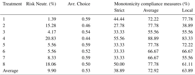
‘Risk Neutr.’ is the percentage of choices which are compatible with risk neutrality, i.e.,q=0.1. ‘Avr. Choice’ is the average choice made by all subjects in each treatment over all panels. The last three columns refer to percentages of subjects fulfilling the monotonicity property at three different levels: ‘Strict’ indicates the percentage of subjects whose choices were all compatible with the monotonicity property; ‘Average’ indicates the percentage of subjects whose choices were on average compatible with the monotonicity property; and ‘Local’ indicates the percentage of subjects whose choice ofqdecreased from panel 1 to panel

2.

From Table 4 it follows that: (i)µ5<µ2andε5<ε2, and (ii)µ6<µ3andε6<ε3. This observation agrees

with the empirical findings of Baye et al. (2003).

5.4. Accounting for Risk Attitudes

We summarize the preceding observations as follows. On the basis of descriptive analysis, the data supports some of the model’s predictions, and rejects others. Given that some of the predictions that the data supports are non-trivial, particularly the consistency test,HC, the underlying Burdett and Judd (1983) and Varian (1980) models are sound. However, there is some factor, the model does not account for, that impacts systematically the way subjects play the game. In the case ofComplete Coveragethis unaccounted factor is qualitatively unimportant. However,

underIncomplete Coveragethis unaccounted factor becomes determinant. The model assumes that subjects are

risk neutral, expected utility maximizers. The unaccounted factor could be the subjects’ risk attitudes.

We have captured two aspects of subjects’ risk attitudes: (i) the average choice over the four panels, and (ii) the “transition” across two subsequent panels. The former can be used as a proxy for a subject’s risk aversion, and the latter as a qualitative variable reflecting a subject’s compliance with the monotonicity property.

Table 5 summarizes the information and descriptive statistics regarding the lottery-choice task for all treat-ments. The second and third columns refer to the percentages of risk neutral subjects: (i) theRisk Neutr. column

indicates the percentage of choices which are compatible with risk neutrality, and (ii) theAvr. Choice column

indicates the average choice by all subjects in the treatment over all panels. The three remaining columns refer to percentages of subjects which comply with the monotonicity property at three different levels: (i) theStrict

column indicates the percentage of subjects whose choices were all compatible with the monotonicity property, (ii) theAveragecolumn indicates the percentage of subjects whose choices were on average compatible with the

monotonicity property, and (iii) theLocalcolumn indicates the percentage of subjects whose choice ofqdecreased

from panel 1 to panel 2, i.e., of individuals that comply with the monotonicity property for the minimum increase in the risk. The purpose of the penultimate column is to allow for human errors which might induce inconsistent transitions from a given panel to the next one. And the purpose of the last column is to help infer the local behavior of the subjects’ utility functions.

The results of the lottery-choice task are summarized in the following two observations:

From Table 5, one concludes the following. Our results confirm previous findings of choice agglomeration around probabilities close to 0.5 (Georgantzís et al., 2003). The average choices exhibit no systematic patterns across treatments. A Kruskal-Wallis test does not reject the homogeneity of the distribution of subjects’ average choices across treatments. Overall, slightly less than 10% of the decisions are compatible with risk neutrality in any of the panels. However, this percentage falls below any significance level if one requires that a subject behaved in a way compatible with risk neutrality in all four panels.

Observation 9. The data does not support the hypothesis that subjects accept more risk in exchange for a

higher expected return.

In Table 5, columnStrict indicates the percentage of the subjects that comply strictly with the monotonicity

property varies across treatments, ranging from 27.7% in treatment 2 to 55.5% in treatment 4. Overall, only 38% of the subjects comply strictly with monotonicity. ColumnAverageindicates the percentage of subjects that comply

on average with the monotonicity property is 72.9%. ColumnLocalindicates the percentage of the subjects whose

choice ofqdecreased from panel 1 to panel 2 is 63.9%.

5.5. Econometric Model

Having established the violation of hypothesesHRNandHM, we assess its impact on the experimental results. We estimate price distributions conditional on experimental design parameter-specific variates, on one hand, and, individual-specific characteristics related to risky choice, on the other hand. From the estimated price distribution we can derive the distributions of both average and minimum prices and assess the impact of experimental design parameters and risk attitudes on these distributions.

We model the observed prices as being generated by beta distributions. The beta distribution is commonly used in the statistical analysis of variables with a bounded support. It is a flexible distribution which can accommodate asymmetries and various distributional shapes: uniform, bell-shaped, U-shaped, J-shaped. As it is a distribution for bounded variables, it naturally incorporates a relation between mean and variance, so that, for unimodal dis-tributions, the variance is lower for beta variables with a mean near the boundaries than for beta variables whose mean lies around the center of the support. Finally, the mathematical tractability of the beta distribution generally puts no excessive burden on the estimation and interpretability of the results.

Our formulation is similar but slightly more general than the one used by Ferrari and Cribari-Neto (2004). We allow some degree of heterogeneity by doing the estimation conditional on a set ofKcovariates,xi= (x1i,x2i, . . . ,xKi)′,

where subscripti=1, . . . ,N indexes the experimental observations. In our analysis, these covariates are related

to the design of each treatment and to the risk attitudes of the subjects. We parametrize a price distribution in terms of its conditional mean,E(p|xi) =Θi=Θ(xi), and a function∆i=∆(xi)related to dispersion.19 Given these

definitions, the probability density function of prices is

f(p|xi) =

Γ₍1/∆_i)

Γ(Θ_i/∆_i)Γ((1−Θ_i)/∆_i)p

Θ_i/∆_i−1_(1−p)(1−Θ_i)/∆_i−1_{, (6)}

where 0≤p≤1, andΓ(·)is the gamma function.

We use the following functional forms for the mean and the dispersion:

Θ_i=Λ(x′_iθ), (7)

∆_i=exp(x_i′δ), (8)

whereΛ(s) =1/(1+e−s)is the logit function, andθ andδ areK-dimensional vectors of unknown parameters.

The functional forms (7) and (8) guarantee thatΘ_i lies between 0 an 1 and∆_i is greater than 0, for all possible