A Bayesian model to correct underestimated 3-D wind speeds from sonic anemometers increases turbulent components of the surface energy balance

www.atmos-meas-tech.net/9/5933/2016/ doi:10.5194/amt-9-5933-2016

© Author(s) 2016. CC Attribution 3.0 License.

A Bayesian model to correct underestimated 3-D wind speeds

from sonic anemometers increases turbulent components

of the surface energy balance

John M. Frank1,2, William J. Massman1, and Brent E. Ewers2

1_{US Forest Service, Rocky Mountain Research Station, 240 W. Prospect Rd., Fort Collins, CO 80526, USA}

2_{University of Wyoming, Department of Botany and Program in Ecology, 1000 E. University Ave, Laramie, WY 82071, USA} Correspondence to:John M. Frank (jfrank@fs.fed.us)

Received: 25 April 2016 – Published in Atmos. Meas. Tech. Discuss.: 23 June 2016

Revised: 17 November 2016 – Accepted: 21 November 2016 – Published: 12 December 2016

Abstract. Sonic anemometers are the principal instruments in micrometeorological studies of turbulence and ecosystem fluxes. Common designs underestimate vertical wind mea-surements because they lack a correction for transducer shad-owing, with no consensus on a suitable correction. We rean-alyze a subset of data collected during field experiments in 2011 and 2013 featuring two or four CSAT3 sonic anemome-ters. We introduce a Bayesian analysis to resolve the three-dimensional correction by optimizing differences between anemometers mounted both vertically and horizontally. A grid of 512 points (_{∼ ±}5◦ resolution in wind location) is defined on a sphere around the sonic anemometer, from which the shadow correction for each transducer pair is de-rived from a set of 138 unique state variables describing the quadrants and borders. Using the Markov chain Monte Carlo (MCMC) method, the Bayesian model proposes new values for each state variable, recalculates the fast-response data set, summarizes the 5 min wind statistics, and accepts the proposed new values based on the probability that they make measurements from vertical and horizontal anemome-ters more equivalent. MCMC chains were constructed for three different prior distributions describing the state vari-ables: no shadow correction, the Kaimal correction for trans-ducer shadowing, and double the Kaimal correction, all ini-tialized with 10 % uncertainty. The final posterior correction did not depend on the prior distribution and revealed both self- and cross-shadowing effects from all transducers. Af-ter correction, the vertical wind velocity and sensible heat flux increased ∼10 % with ∼2 % uncertainty, which was significantly higher than the Kaimal correction. We applied

the posterior correction to eddy-covariance data from vari-ous sites across North America and found that the turbulent components of the energy balance (sensible plus latent heat flux) increased on average between 8 and 12 %, with an aver-age 95 % credible interval between 6 and 14 %. Considering this is the most common sonic anemometer in the AmeriFlux network and is found widely within FLUXNET, these results provide a mechanistic explanation for much of the energy im-balance at these sites where all terrestrial/atmospheric fluxes of mass and energy are likely underestimated.

Copyright statement

This paper was written and prepared by a US Government employee on official time, and therefore it is in the public domain and not subject to copyright.

1 Introduction

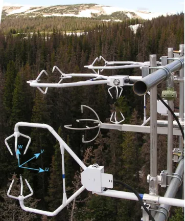
mi-Figure 1. Photograph of the 2011 experiment with two CSAT3 sonic anemometers mounted vertically and two horizontally. The cardinalu,v, andwaxes are shown in light blue near one of the vertical instruments. Figure from Frank et al. (2013).

crometeorology and ecosystem flux communities that many sonic anemometers, the core instrument for all modern eddy-covariance systems, systematically underestimate the verti-cal wind component (Frank et al., 2016; Horst et al., 2015; Kochendorfer et al., 2012). The ramifications for this are that all vertical fluxes (i.e., carbon dioxide, water vapor, latent heat, sensible heat, momentum) are similarly underestimated for any ecosystem. This underestimate is roughly consistent with the persistent energy balance closure problem across flux sites (Leuning et al., 2012; Stoy et al., 2013; Wilson et al., 2002), where a vast majority are assumed to be system-atic biased towards low turbulent fluxes of sensible and latent heat.

Horst et al. (2015) and Frank et al. (2016) have shown that the error in at least two non-orthogonal sonic anemometer designs can be traced to transducer shadowing that remains uncorrected in the anemometer’s firmware. In both studies, shadowing was described a priori by theoretical formulations based on the wind tunnel tests of Kaimal (1979), yet there was no consensus on a correction. A shortcoming in the use of formulations derived for single transducer pairs in lami-nar flow to describe turbulent flow distortions around more complex geometries (Fig. 1) is that shadowing between all transducers and structures cannot be accurately represented

or incorporated. A second problem is that in turbulent flow fields there are few standards available to use as a calibration reference. Advancements in Bayesian techniques (Gelman et al., 2014) have created the potential to resolve both of these issues by incorporating prior knowledge of transducer flow distortions with a model that evaluates the omnidirectionality of a sonic anemometer to produce a posterior 3-D correction. To quantify a 3-D correction of the CSAT3 sonic anemometer, we reanalyze data from field experiments con-ducted by Frank et al. (2013, 2016), where wind measure-ments from non-orthogonal anemometers mounted vertically and horizontally were significantly different. We develop a Bayesian hierarchical model to evaluate three hypotheses:

1. A 3-D shadowing correction based solely on wind loca-tion can make a non-orthogonal sonic anemometer om-nidirectional.

2. This correction increases vertical wind measurements more than expected from single transducer shadowing because it accurately represents all shadowing between transducers.

3. In ecosystems where these instruments are deployed, the application of this correction will result in signif-icantly higher Bayesian credible intervals for the tur-bulent components of the energy budget and improved surface energy budget closure.

2 Methods

2.1 Reanalysis of field experiments

Table 1.Summary of the subset of data from Frank et al. (2013, 2016) reanalyzed in this study listing the four CSAT3 anemometers (A–D), their location within the five-position horizontal array, and whether they are mounted horizontally (∗). Because processing the Bayesian model is extremely intensive, only 5 % of the available data were reanalyzed.

Position Number of 5 min periods

Dates 1 2 3 4 5 Available Reanalyzed

5–19 July 2011 A∗ B – C D∗ 2520 126

19–26 July 2011 A B∗ – C∗ D 1992 100

9–16 August 2011 B∗ A – D C∗ 1974 98

16–22 August 2011 B A∗ – D∗ C 1620 81

26–30 July 2013 A∗ – B – – 906 46

23–27 August 2013 – – A – B∗ 1050 52

6–24 September 2013 – – B D∗ – 498 25

Finally, because our Bayesian model is computationally in-tensive, we reanalyze a subset of only 5 % of the available data (see Sect. 2.3).

2.2 The Bayesian model

Bayesian statistics is based on Bayes’ theorem (Bayes and Price, 1763), which in modern applications relates the poste-rior probability of a model parameter conditioned on data to the product of the likelihood of the data and the prior prob-ability of that parameter (Gelman et al., 2014). In essence, the prior represents an initial educated guess or belief in the value of a model parameter; the likelihood is the prob-ability of observing the data if they were deterministically generated from a model; and the posterior is an updated belief in the model parameter considering each the prior, the model, and the data. Analytical evaluation of the pos-terior is rarely possible, as is in our case; thus the poste-rior is commonly estimate through the Markov chain Monte Carlo (MCMC) method, Gibbs sampling (Appendix A1), and the Metropolis–Hastings algorithm (Kruschke, 2010). The framework of our Bayesian model is to divide the sphere around the sonic anemometer into approximately equal grid points and to define a prior probability distribution of the 3-D shadowing correction for each transducer pair at each lo-cation. Then, the model proposes new corrections for each grid point, recalculates the fast-response data set, summa-rizes new 5 min wind statistics, determines the probability that the updated measurements from vertical and horizontal anemometers are more equivalent using the proposed correc-tion versus the old one (i.e., the Metropolis–Hastings ratio, which is Eq. A13 evaluated for the proposed versus old cor-rection), and finally accepts/rejects the proposal probabilisti-cally from this ratio to construct the posterior correction. The model recursively adjusts the distribution that generates the proposals to achieve between 25 and 50 % acceptance rates, which are theoretically optimal (Gelman et al., 2014). We de-fine a grid of 512 points (∼ ±5◦resolution of wind location) on a sphere around each of the three transducer pairs of the sonic anemometer. Neglecting the upper and lower

mount-ing arms that extend back into the electronics housmount-ing and support block, the CSAT3 is symmetrical on either side of a transducer pair, between the upper and lower hemispheres, and for each of the three transducer pairs. To pool data and reduce computations, we make these assumptions of symme-try to describe all 1536 points from a set of 138 unique state variables.

In our mathematical notation, we use uppercase and lower-case subscripts to distinguish variables as scalars, vectors, or matrices. Uppercase subscripts are part of the variable name, denote the dimensionality of the variable, and describe the coordinate system. For example,MS×T is a two-dimensional

matrix with dimensionsSandT, which correspond to sonic and transducer coordinates; since there are three dimensions for both coordinate systems, this is a 3×3 matrix. One up-percase subscript by itself denotes a vector in that coordinate system. Lowercase subscripts denote indexing for variables that are defined for multiple times or replicate anemome-ters; these are essentially multidimensional arrays. When the same letter appears as both an uppercase and lowercase sub-script, this refers to thecth element of dimensionC.

We test three prior corrections: no shadow correction, the Kaimal correction (Kaimal, 1979; Frank et al., 2016; Horst et al., 2015), and a doubling of the Kaimal correc-tion (Frank et al., 2016). The Kaimal correccorrec-tion is defined as

UTt =(1−0.16+0.16θ/70)U´Tt forθ≤70◦andUTt = ´UTt

for θ >70◦, where UT andU´T are the measured and cor-rected wind velocities in transducer coordinates andθ is the angle between the wind and the transducer acoustic path,t.

The model predicts the standard deviation of the data in cardinal coordinates,σC, which is defined during each 5 min period,f, for each replicate sonic anemometer, i (Fig. 1), from a normal distribution with meanσ_ˆCand standard devi-ationε(Eq. 1).

σCc,f,i∼N

ˆ

σCc,f,i, ε−

2 ₍₁₎

matter if each grid point is independent or that they linked together through symmetry.αTis given a normal prior proba-bility distribution with mean equal to the prior correction,P, evaluated for each transducer pair for wind blowing through the longitude, λ, and latitude,ϕ, associated with each grid point and with a predefined standard deviation equal to 0.1, or±10 % uncertainty (Eq. 2).

αTt,g∼N

P (t, g),0.1−2 (2)

The 3-D correction is applied to every 20 Hz sample, j, of the original measured wind velocity data in transducer co-ordinates,UT. The nominal predictor variable,h, selects the corresponding grid point that occurs with every 20 Hz sam-ple. The corrected 20 Hz wind velocity in transducer coordi-nates isU´T(Eq. 3).

´

UTf,i,j=UTf,i,j·αTh (3)

The non-orthogonal data are transformed via matrix mul-tiplication into orthogonal sonic coordinates,U´S(Eq. 4).

´

USf,i,j =MS×TU´Tf,i,j (4)

The matrix, MS×T, is specific to the CSAT3 geometry

(Eq. 5).

MS_×T =

       −4 3 2 3 2 3

0 √2

3 −

2

√

3 2

3√3 2 3√3

2 3√3

       (5) = 

 −1

.333 0.667 0.667 0 1.155 −1.155 0.385 0.385 0.385

 

For the model to predict data simultaneously from both vertical and horizontal anemometers, a final corrected time series data set is produced in cardinal coordinates,U´C

´

UCf,i,j=NC×SoUS´ f,i,j (6)

The matrixNC×Sis straightforward (Eq. 7), and the nominal

predictor variable,o, selects the orientation of every 20 Hz sample.

NC×So=                

 10 01 00

0 0 1



, o₌1 (i.e., vertical)



 10 00 −01

0 1 0



, o₌2 (i.e., horizontal) (7)

Using the corrected time series data in cardinal coordi-nates, the model calculates the average correction along the

three dimensions,βC, for the 5 min standard deviation data for each anemometer (Eq. 8).

βCf,i= v u u

t 1

J−1

J

P

j=1

´

UCf,i,j−

1

J J

P

j=1

´

UCf,i,j

!2

v u u

t 1

J−1

J

P

j=1

UCf,i,j−

1

J J

P

j=1

UCf,i,j

!2 (8)

Equation (8) is equivalent to the ratio of the standard de-viation ofU´Cdivided by the standard deviation ofUC, eval-uated during each 5 min period for each sonic anemometer. The reference condition for every 5 min period,eσC, is a state variable representing the “true” standard deviation of wind velocity. It is assigned a uniform prior probability distribu-tion that generously includes the true value by allowing each

eσCto range from 0 to the maximum of allUCmeasurements (Eq. 9).

eσCc,f ∼Unif(0,max(UC)) (9)

Finally, the model predicts the mean for the standard devi-ation data as the reference divided by the average correction (Eq. 10).

ˆ σCf,i=

eσCf

βCf,i

(10)

To complete the Bayesian model definition, the model er-ror is a state variable which is assigned a prior probability distribution with a gamma distribution (Eq. 11).

ε_∼Ŵ(1,b)´ (11)

The variance of the gamma distribution,b´, is assigned the same variance as the prior distribution foreσCwhich is a uni-form distribution (Eq. 12).

´

b₌

√

12 max(UC)−0

(12) Distributions are defined where normal distributions are

θ_∼N (a, b) with expected value E(θ )₌a and variance var(θ )₌1/b2, gamma distributions are θ_∼Ŵ(a, b) with

E(θ )₌a/b and var(θ )₌a/b2, and uniform distributions areθ_∼Unif(a,b)withE(θ )₌(a₊b)/2 and var(θ )₌(b₋ a)2/12.

2.3 Analysis

Table 2.Increase inH₊LE (sum of the turbulent components of the energy balance, i.e., sensible and latent heat flux) at various sites across North America after applying shadow correction to the CSAT3 time series data.

Percent change after applying shadow correction

Posterior correction

Site Coordinates Dates Height (m) Kaimal correction mean_±SD∗

Yuma, AZ, 33◦5′N 6–15 June 8.25 5.1 % 9.8±2.3 %

USA 114◦32′W 2008 [5.1, 14.8 %]

Yuma, AZ, 33◦5′N 5–14 June 2.00 4.5 % 9.4±2.8 %

USA 114◦32′W 2009 [3.1, 16.1 %]

Fraser, CO, 39◦53′48.23′′ N 5–14 April 27.50 5.6 % 9.9±1.4 %

USA 105◦53′33.87′′W 2015 [7.4, 12.2 %]

Fraser, CO, 39◦53′48.23′′N 5–14 April 6.40 6.8 % 11.6_±1.2 %

USA 105◦53′33.87′′W 2015 [9.4, 13.9 %]

Beltsville, MD, 39◦1′51.23′′N 16–31 July 4.00 5.5 % 10.4_±2.1 %

USA 76◦50′39.40′′W 2014 [6.3, 14.8 %]

Glacier Peak, WY, 41◦22′52′′N 28 August– 3.20 5.3 % 11.3±3.1 %

USA 106◦15′47′′W 8 September 2015 [4.6, 19.2 %]

Agua Salud, 9◦13′31.65′′N 6–16 November 5.00 4.7 % 8.1±1.6 %

Panama 79◦45′36.41′′W 2015 [5.3, 10.8 %]

SD: standard deviation;∗[95 % credible interval].

(see discussion in Sect. 4.1), we normalized each chain. This was done in post-processing by dividing αT by the average ofαTafter each time one of the 138 state variables was up-dated within each MCMC step. We inspected each chain us-ing trace plots, removed the first 500 steps for burn-in, and kept 1 out of every 140 steps to eliminate autocorrelation between steps for most grid points (even after reducing to 138 state variables, a few of these were estimated from rel-atively fewer data, which unavoidably led to high autocor-relation between steps). This reduced each MCMC chain to 68 steps. We conducted several preliminary Bayesian analy-ses and used trace plots and tests for autocorrelation to de-termine that 10 000 steps was sufficient for convergence for most of the 138 state variables defining αT. Most of these parameters required little or no thinning to reduce autocor-relation between steps and could have remained as MCMC chains with 1000–10 000 steps. Yet, since the goal was to create a complete 3-D correction, we decided to thin all state variables equally. Even though diagnostic tests showed that all parameters, including those with high autocorrelation, ap-peared to converge within 10 000 steps, it is possible that these chains are still too short for proper convergence. One safeguard against this is confirming that the results from the three chains all result in similar posterior distributions (see Sect. 3.3).

Because each MCMC chain was based on a different prior, they are not replicate chains from the same Bayesian analysis. Instead, these are three separate solutions for the posterior correction. But after considering the results (see Sect. 3.3) and recognizing that, apart from normalization, the prior had minimal influence on the solution, we combined

the three priors to create a single chain containing 204 in-dependent samples of the posterior correction. We rescaled the correction to be absolute by forcing the condition that the correction will not change, on average, equatorial wind measurements (i.e., (u2+v2)1/2; see discussion in Sect. 4.1). This was done by (1) applying the normalized correction to the time series of vertically mounted anemometers, (2) calcu-lating the corrected 5 min standard deviations for equatorial winds, (3) performing linear regression without an intercept (i.e., model the average change in equatorial winds solely as a scaling factor) between the corrected and uncorrected stan-dard deviations, (4) repeating this for each of the 204 pos-terior samples, and (5) determining the average of the 204 regression slopes. We divided all values in the normalized 3-D correction by this average scaling factor to produce our final posterior correction.

grid points and 5 % of the original data were optimal consid-ering these processing constraints.

There is a slight distinction to be made between the prior corrections – which are defined as a function, αT(λ, ϕ), of the true longitude and latitude of the wind – and the posterior correction, which is a function,αT eλ,eϕ

, where∼represents the uncorrected sonic anemometer measurement of wind lo-cation. This distinction means the posterior correction can be applied directly to the uncorrected raw data, whereas the prior should be applied iteratively (i.e., start with the uncor-rected observed wind, determine the correction, update the wind measurement, determine the new wind location, update the correction, etc.). To directly compare the prior and poste-rior corrections, we also present our posteposte-rior correction with the wind locations recursively adjusted to approximate the true longitude and latitude. For these analyses, we smoothed the posterior spatially across the grid points with a spheri-cal spline fit (Wahba, 1981) using R package mgcv (Wood, 2006).

We quantified the impact of shadowing on measurements of the standard deviations of winds in the three dimensions and the sensible heat flux (H). This was done iteratively (i.e., for each of the 204 posterior samples) by (1) apply-ing the posterior correction to the raw data of vertically mounted anemometers, (2) calculating the 5 min measure-ments, and (3) performing linear regression without an inter-cept between the corrected and uncorrected measurements. The 204 regression slopes were combined to form a distri-bution describing the relative change in each of these mea-surements due to shadowing. ForH, the data were planar-fit-rotated (Lee et al., 2004), time-lag-adjusted, and vapor-flux-corrected (Massman and Lee, 2002) using ancillary data from the GLEES AmeriFlux site (Frank et al., 2014).

Finally, we quantified the impact of the 3-D correction on the sum of the turbulent components of the energy balance (i.e., sensible and latent (LE) heat flux) at various sites across North America (Table 2). Each site featured a CSAT3, a fast-response hygrometer, and ancillary meteorological data. Measurements of LE were calculated similar to H but in-cluding the Webb–Pearman–Leuning correction (Webb et al., 1980). The impact of the 3-D correction was quantified as a distribution similar to above, except compiled from 30 min time periods.

2.4 Validation experiment

We conducted a validation experiment of the posterior 3-D correction at the Colorado State University, Agricultural Re-search Development and Education Center (ARDEC), Fort Collins, CO, USA (40◦39′7.9′′N, 104◦59′45.7′′W), from 7 to 14 October 2016. Three CSAT3 sonic anemometers were mounted on an east–west boom 2 m above a pasture of short grass and∼36 m south of a mature corn field. Typical winds at this site are from the north, so in this experiment we refer to cardinalu,v, andw, where the measurements have been

-40 -20 0 20 40

(a) σ_u, RMSE=4.6 %

-40 -20 0 20 40

Percent error in

σ

between two vertical anemometers (%)

(c) σ_v, RMSE =3.7 %

0 1 2 3

-40 -20 0 20 40

(e) σ_w, RMSE=3.3 %

-40 -20 0 20 40 (b) σ_u, RMSE=8.4 %

-40 -20 0 20 40

Percent error in

σ

between a horizontal and vertical anemometer (%)

(d) σ_v, RMSE=11.1 %

0 1 2 3

-40 -20 0 20 40 (f) σ _w, RMSE=8.5 %

σ (m s-1₎

Figure 2.Uncorrected measurements of the 5 min standard devia-tion of wind (σ) along the cardinal(a, b)u,(c, d)v, and(e, f)w axes are not equivalent between vertically and horizontally mounted CSAT3 sonic anemometers. Data from an ideal 3-D anemometer would have similar percent errors between a horizontal and a ver-tical anemometer(b, d, f)to those found between two anemome-ters mounted vertically(a, c, e). The data are from 2011 and 2013 field experiments at the GLEES AmeriFlux site (Frank et al., 2016, 2013). The 2011 data in panels(b),(d), and(f)are randomly paired between the two anemometers in different orientations. Results are summarized as root mean square error (RMSE).

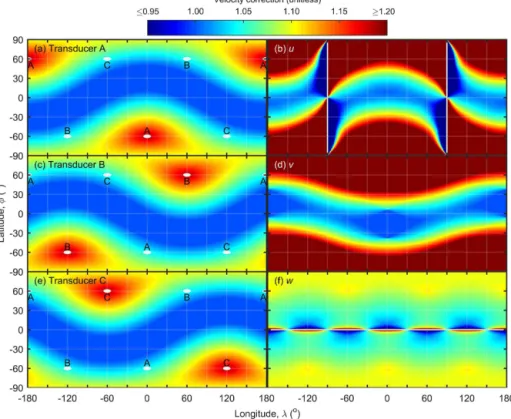
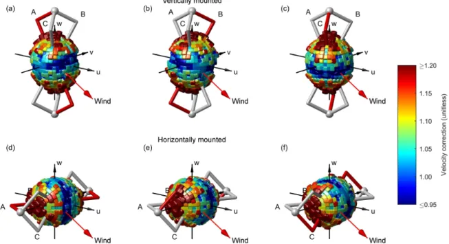
be-Figure 3.The Kaimal correction, one of three priors tested in this study, for the(a)A,(c)B, and(e)C transducer pairs, each represented by a white dot, of a CSAT3 sonic anemometer accounts for self-shadowing but not cross-shadowing between transducers. The same correction expressed in sonic anemometer coordinates(b)u,(d)v, and(f)wshows that, for near-equatorial winds, minimal correction is required for the horizontal wind components, while significant correction and instability exist in the vertical wind componentw. Longitude and latitude are relative to theuaxis (Fig. 1).

tween anemometers are presented as root mean square of the relative error (RMSE) between measurements from the ma-nipulated anemometers and the vertically mounted one.

3 Results

3.1 No correction

Without any shadow correction applied, measurements be-tween a vertically and a horizontally mounted anemome-ter were different, which becomes clear when the variance between two vertical anemometers is taken into account (Fig. 2b, d, f vs. a, c, e). The RMSE in the 5 min standard deviation of wind along all cardinal dimensions (u,v, and w)combined was 9.4 % between a vertical and a horizontal anemometer, whereas the same metric between two vertical anemometers was 3.9 %. The largest discrepancy was along the cardinal vaxis, where the RMSE increased from 3.7 to 11.1 % when comparing vertical and horizontal anemometers (Fig. 2c vs. d).

3.2 The Kaimal prior correction

-40 -20 0 20 40

(a) σ_u, RMSE=4.7 %

-40 -20 0 20 40

Percent error in

σ

between two vertical anemometers (%)

(c) σ_v, RMSE=3.6 %

0 1 2 3

-40 -20 0 20 40

(e) σ_w, RMSE=3.4 %

-40 -20 0 20 40 (b) σ_u, RMSE=5.4 %

-40 -20 0 20 40

Percent error in

σ

between a horizontal and vertical anemometer (%)

(d) σ_v, RMSE=6.6 %

0 1 2 3

-40 -20 0 20 40 (f) σ_w, RMSE=6.7 %

σ (m s-1

)

Figure 4.Kaimal-corrected measurements (i.e., one of three priors tested) of the 5 min standard deviation of wind (σ) along the cardi-nal(a, b)u,(c, d)v, and(e, f)waxes are more equivalent between vertically and horizontally mounted sonic anemometers. The per-cent errors between a horizontal and a vertical anemometer(b, d, f)

are smaller for all three cardinal dimensions than they were for the uncorrected data (Fig. 2) and are more similar to those found be-tween two anemometers mounted vertically(a, c, e). The data are from 2011 and 2013 field experiments at the GLEES AmeriFlux site (Frank et al., 2016, 2013). The 2011 data in panels(b),(d), and

(f)are randomly paired between the two anemometers in different orientations. Results are summarized as RMSE.

3.3 The Bayesian model

Figure 5 illustrates the approach of the Bayesian model. The model initializes the 512 grid points with a prior, in this case the Kaimal correction. No matter the transducer pair or vertical versus horizontal mounting, the 3-D corrections for all cases are identical but rotated versions of a com-mon correction based on 138 unique state variables. For a single instantaneous wind, the simultaneous corrections for all six combinations of transducer pairs and mounting ori-entations will be different. As the MCMC chains progress, the Bayesian model will continuously adjust each of the 138 unique state variables so that measurements from the verti-cally and horizontally mounted anemometers are most sim-ilar based on the univariate conditional posterior probabil-ity distribution (Eq. A13). Much of the predictive power of the model comes from resolving the inconsistencies along the cardinal v axis (Fig. 2d), where vertically and horizon-tally mounted anemometers are likely to be most dissimi-lar. Specifically, a vertically mounted CSAT3 should

mea-sure reasonably correct cross winds, which must flow across the entire transducer and support structure of a horizontally mounted CSAT3.

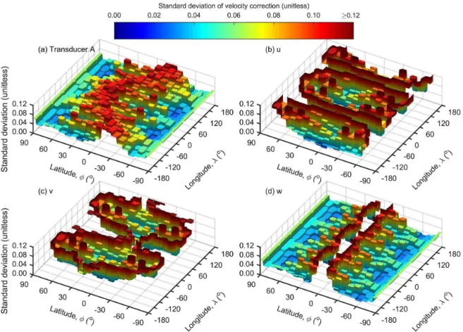
Each MCMC chain was initialized with the mean of each prior, yet after convergence their posterior corrections were remarkably similar regardless of the choice of prior correc-tion, with one peculiarity (Fig. 6). There was a clear linear relationship between the prior correction averaged across all 512 grid points (1.000 for no correction, 1.040 for the Kaimal correction, and 1.080 for the double-Kaimal correction) and the magnitude of the posterior correction (1.030, 1.064, and 1.098, respectively) that relates to the Bayesian model esti-mating a relative and not absolute correction (see discussion in Sect. 4.1). The posterior correction is more than an esti-mate of the optimal solution, as it intrinsically accounts for the uncertainty of the correction at each of the 512 grid points (Fig. 7). Whereas each prior was defined with 10 % uncer-tainty (Eq. 2), much of the posterior correction has much lower standard deviations, especially around the transducers where values were as low as 2.5 % (Fig. 7a). These uncer-tainties can be expressed in sonic coordinates for theu,v, andwcomponents, which in general show that the posterior correction is most certain for winds along each of those axes (Fig. 7b–d), with the uncertainty along thewmeasurement ranging from 2.7 to 18.3 %.

Figure 8 illustrates the completion of the Bayesian model where the same posterior correction is applied to all trans-ducer pairs and both mounting orientations. For every instan-taneous wind, application of these six different corrections ultimately results in the 5 min standard deviations of wind along the cardinalu,v, andw axes being most similar be-tween the two mounting orientations.

3.4 The posterior correction

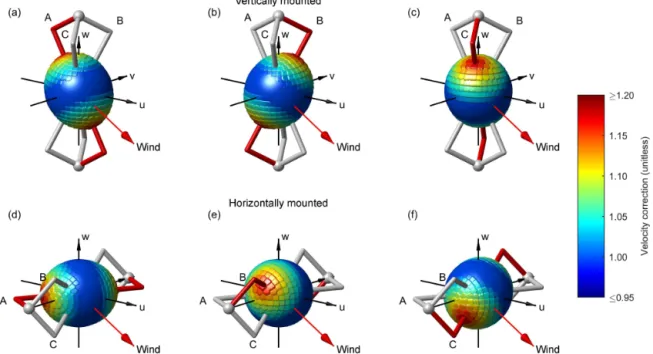
Figure 5.The Kaimal correction, one of three priors tested in this study, evaluated among 512 cells for the(a, d)A,(b, e)B, and(c, f)C transducer pairs of the CSAT3 sonic anemometer mounted either in the(a–c)typically vertical or(d–f)experimentally horizontal orientations. Though the correction is identical relative to all transducer pairs, the same instantaneous wind results in different corrections depending on the transducer pair and the orientation.

mounted anemometers (Fig. 10), where the RMSE for all car-dinal dimensions combined was 5.3 %, or 1.36 times greater than the same error between two vertical anemometers. The discrepancy along the cardinalvaxis was further reduced to 4.4 %, which is only 1.20 times greater than the same error for two vertical anemometers, and the bias has been removed (Fig. 10d vs. 4d). When the posterior correction was applied to the vertically mounted anemometers, there were similar increases to the Kaimal correction in the 5 min standard de-viations ofuandv(0.6±0.8 [−1.0, 2.2] %, 2.7±0.7 [1.5, 4.1] %, mean±standard deviation [95 % credible interval], Fig. 11a–b). But compared to the Kaimal correction, the in-creases inw(10.6±1.7 [7.6, 13.9] %) andH(9.9±1.6 [7.2, 12.6] %) were substantial and significantly higher (Fig. 11c– d). We provide the MCMC chain for the final posterior cor-rection in the Supplement as a tool for researchers to eval-uate in other sonic anemometer studies, to examine the un-certainty in ecosystem flux measurements, and to investigate surface energy balance closure.

3.5 Turbulent components of the ecosystem energy balance across a continent

We applied the posterior correction to various sites across North America that deploy the CSAT3 in their eddy-covariance instrumentation (Table 2). The estimated increase in H₊LE at these sites ranged from 8.1 to 11.6 % with an average standard deviation and 95 % credible interval of

±1.9 % and 6.1–13.8 %, respectively. For all but one site, the

increase inH₊LE was significantly higher than the increase due to the Kaimal correction. At the 2 m Yuma, AZ site, the lack of significance is related to anomalously low instanta-neous wind latitudes for which thewcorrection is most un-certain (Fig. 7d).

3.6 Validation of the posterior correction

The validation experiment was conducted during excellent fall weather with no precipitation, where winds averaged 2.0±1.2 m s−1, maximum sustained gusts were 7.8 m s−1, 38 % of the winds were from the northeast (45◦) to north-northwest (337.5◦), 25 % of the winds were from the southeast (135◦) to south (180◦), and during the other times there were some occasional westerly winds. Results are summarized in Table 3. The RMSE differences be-tween a horizontally mounted anemometer and a vertically mounted anemometer were large (12.6–16.5 %) for uncor-rected measurements. Applying the Kaimal correction to these anemometers reduced the RMSE differences in σu

andσv (8.5 and 11.4 %) but increased the difference in σw

(17.5 %). Compared to the uncorrected data, the average pos-terior correction decreased the RMSE differences in all di-rections, though only the reduction inσv (8.0–12.2 %) was

statistically lower (i.e., 95 % credible interval). Compared to the Kaimal correction, the average posterior correction was larger forσu but lower forσv andσw, with the

reduc-tion inσw (11.8–15.9 %) being statistically lower than with

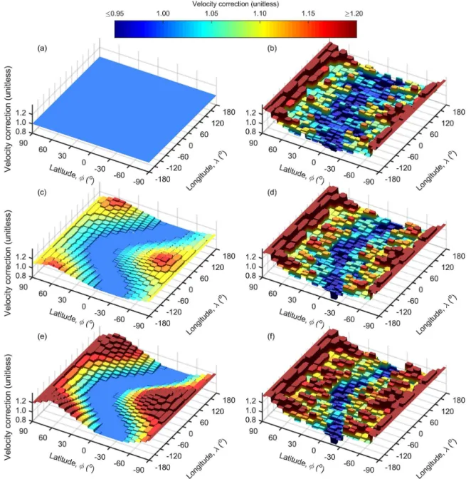
Figure 6.The A transducer pair correction evaluated among 512 cells for the three prior corrections tested in this study:(a)flat,(c)Kaimal, and(e)double Kaimal, with their corresponding unnormalized posterior corrections(b),(d), and(f), respectively. All posteriors have similar relative topography. They differ in absolute scaling, where priors with higher absolute magnitude result in posteriors with higher absolute magnitude, which is apparent from the different colorings.

an askew-mounted anemometer and a vertically mounted anemometer were small/moderate for σu and σv (6.7 and

11.3 %) and large forσw (14.7 %) for uncorrected

measure-ments. Applying the Kaimal correction to these anemometers reduced the RMSE differences in all directions (4.4–13.5 %). The standard deviations for the RMSE differences using the posterior correction were higher for the askew manipulation (1.5–2.4 %) than they were for the horizontal manipulation (1.1–1.3 %). Compared to the uncorrected data, the average posterior correction increased the RMSE difference for σu

(8.6 %) but decreased the differences for σv andσw (10.3

and 13.9 %), though none of these changes were statistically significant. Compared to the Kaimal correction, the average posterior correction increased the RMSE differences for all directions, with the differences in σu (6.2–11.6 %) andσv

Figure 7.Standard deviations of the posterior correction for(a)the A transducer pair and the wind velocities(b)u,(c)v, and(d)w. When compared to the standard deviation of the prior which was defined as 0.1, the transducer correction is more certain in regions with higher topography (Fig. 6). The results in CSAT3 sonic coordinates reflect both the uncertainty in the transducer correction plus cancelation and amplification of errors due to the coordinate transformation. The posterior correction foru,v, andwis most certain for winds along theu, v, andwaxes, respectively.

Table 3. Results of a validation experiment of CSAT3 sonic anemometers at ARDEC, CO, showing the relative error in 5 min standard deviation of wind (σ) along the cardinalu,v, andwaxes between a vertical instrument and one mounted horizontal and one mounted askew. All anemometers were compared uncorrected, with the Kaimal correction, and with the posterior correction.

RMSE inσbetween a

manipulated and vertical anemometer (%)

Manipulation Cardinal Uncorrected Kaimal Posterior correction

measurement correction mean±SD∗

Horizontal σu 12.6 % 8.5 % 10.5±1.3 %

[8.4, 13.4 %]

σv 16.5 % 11.4 % 9.8±1.1 %

[8.0, 12.2 %]

σw 15.0 % 17.5 % 13.4±1.1 %

[11.8, 15.9 %]

Askew σu 6.7 % 4.4 % 8.6±1.5 %

[6.2, 11.6 %]

σv 11.3 % 6.0 % 10.3±1.7 %

[7.2, 13.5 %]

σw 14.7 % 13.5 % 13.9±2.4 %

[9.9, 19.4 %]

Figure 8.The posterior correction evaluated for the(a, d)A,(b, e)B, and(c, f)C transducer pairs of the CSAT3 sonic anemometer mounted either in the(a–c)typically vertical or(d–f)experimentally horizontal orientations. The correction is identical relative to all transducer pairs and is constructed from 512 cells with 138 unique values. The Bayesian model adjusts these values to simultaneously correct the same instantaneous wind measured from different transducer pairs and orientations in order to produce similar cardinalu,v, andwwind statistics (Fig. 10).

4 Discussion

4.1 An omnidirectional standard

Perhaps the most important shortcoming in almost every sonic anemometer study is the lack of a standard wind mea-surement to compare against. A fundamental problem is that the principle of sonic measurements (Barrett and Suomi, 1949; Kaimal and Businger, 1963) involves the observer ef-fect; i.e., it is virtually impossible for sonic transducers to ob-serve air parcels without influencing them (Buks et al., 1998). Thus, any method that relies on a sonic anemometer mea-surement as an absolute standard is flawed to an extent. And while we are justified to believe that some sonic anemome-ter measurements are more accurate that others (Frank et al., 2016), it is tenuous to choose any sonic anemometer measurement as a standard. Then, what are the alternatives? Wind tunnels are extremely useful (Horst et al., 2015; van der Molen et al., 2004), yet it is debatable that such lami-nar or quasi-lamilami-nar calibrations are transferrable to turbu-lent field conditions (Hogstrom and Smedman, 2004). And, while other new technologies such as Doppler Lidar exist (Sathe et al., 2011; Dellwik et al., 2015), their application as a field reference standard has been limited.

What we address is the general problem of determining a calibration given an unknown standard or nothing to compare against. Whether this problem exists in medicine (Lu et al., 1997), acoustics (MacLean, 1940; Monnier et al., 2012), or

micrometeorology with respect to calibrating sonic anemom-etry in turbulent flow fields, all approaches have a com-monality of testing the relative consistency of a response to unknown signals. In our situation, we hold the 3-D sonic anemometer to an omnidirectional standard of relative con-sistency and contend that the correction that best achieves this standard is statistically the most likely 3-D calibration. A CSAT3 without any 3-D shadow correction is clearly not omnidirectional (Fig. 2) as measurements depend on the in-strument’s orientation. A CSAT3 with the Kaimal transducer shadow correction is better at meeting this standard (Fig. 4). However, the posterior 3-D correction is remarkably effec-tive in making the CSAT3 omnidirectional (Fig. 10). Because the posterior correction closely achieves the omnidirectional standard, we support our first hypothesis and argue that it is the most accurate correction, in general, for the three dimen-sions of the CSAT3. Whether or not the posterior correction reveals meaningful information regarding vertical winds and turbulent fluxes is another matter discussed below.

es-Figure 9.The posterior correction for the(a)A,(c)B, and(e)C transducer pairs, each represented by a white dot, of a CSAT3 sonic anemometer accounts for both self-shadowing and cross-shadowing between transducers. The same correction expressed in sonic anemome-ter coordinates(b)u,(d)v, and(f)wshows that, for near-equatorial winds, minimal correction is required for the horizontal wind compo-nents, while even more correction exists in the vertical wind componentwthan was present with the Kaimal correction (Fig. 3f). Longitude and latitude are relative to theuaxis (Fig. 1).

timates foreσC andαT only have meaning relative to each

other. This issue is confounded by the choice of prior distri-butions, which vary dramatically in shape but produce simi-lar posteriors except for differences in their absolute magni-tudes (Fig. 6); i.e., higher magnitude priors produce higher magnitude posteriors. Which absolute magnitude is correct? Without specifying an absolute standard, the answer is none of them. To facilitate comparison and combination of the posteriors, we normalized the three MCMC chains.

There is a clear need to specify an absolute standard to reference our results. Without one, our normalized posterior correction reduced the 5 min standard deviations for equato-rial winds (i.e., theu–vplane) by 7 %. Does this make phys-ical sense? No. The idea that equatorial winds should not be changed is consistent with the expectation that the CSAT3 accurately measures equatorial winds, something that has been demonstrated in both wind tunnels and field campaigns (Yahaya and Frangi, 2004; Friebel et al., 2009). Even the Kaimal correction, which is an absolute correction, predicts

<0.1 % error in our measurements of equatorial winds. Be-cause the omnidirectional standard is only relative, we im-pose an additional absolute standard by defining the aver-age correction for equatorial winds to be 0, which is simply achieved by scaling the normalized posterior correction by

7 %. While there certainly is some leeway in this constraint, if the normalized posterior correction were scaled by any-thing other than 7±1.4 % then the correction to horizontal winds would be significantly different (95 % credible inter-val) than both 0 and the Kaimal correction (Fig. 11a–b) and would run counter to our belief that the CSAT3 makes rea-sonably accurate measurements of horizontal winds. 4.2 Impact on vertical wind measurements and

sensible heat flux

-40 -20 0 20 40

(a) σ

u, RMSE=4.7 %

-40 -20 0 20 40

Percent error in

σ

between two vertical anemometers (%)

(c) σ

v, RMSE=3.7 %

0 1 2 3 -40

-20 0 20 40

(e) σ

w, RMSE=3.3 %

-40 -20 0 20 40

(b) σ

u, RMSE=5.5 %

-40 -20 0 20 40

Percent error in

σ

between a horizontal and vertical anemometer (%)

(d) σ

v, RMSE=4.4 %

0 1 2 3 -40 -20 0 20 40

(f) σ

w, RMSE=6.0 %

σ (m s-1)

Figure 10.Posterior-corrected measurements of the 5 min standard deviation of wind (σ) along the cardinal (a, b) u, (c, d)v, and

(e, f) waxes are most equivalent between vertically and horizon-tally mounted sonic anemometers than with either the uncorrected (Fig. 2) or Kaimal-corrected data (Fig. 4). The percent errors be-tween a horizontal and a vertical anemometer are small(b, d, f), especially for the cardinal v dimension (d), and are similar to those found between two anemometers mounted vertically(a, c, e). The data are from 2011 and 2013 field experiments at the GLEES AmeriFlux site (Frank et al., 2016, 2013). The 2011 data in pan-els(b),(d), and(f)are randomly paired between the two anemome-ters in different orientations. Results are summarized as RMSE. The red lines are 95 % credible intervals.

not the Kaimal correction is sufficient is a matter of debate, but it currently represents the best prior knowledge to explain the CSAT3’s shortcomings.

Solely the fact that the posterior correction makes the CSAT3 more omnidirectional does not imply that field mea-surements of vertical wind and turbulent fluxes are impacted, nor does this assure that these impacts would be due to any-thing more than chance. Even with the uncertainty in the pos-teriorwcorrection explicitly quantified (Fig. 7d), it is diffi-cult to foresee ifwis significantly impacted without applying the posterior correction to actual data. A powerful attribute of the Bayesian analysis is that the posterior correction can be applied to raw data to produce probability distribution es-timates for w andH from which statistical inferences can be made. Using GLEES data, Fig. 11c–d confirms that to achieve an omnidirectional sensor (Fig. 10) with minimal change to horizontal winds (Fig. 11a–b) the required correc-tion will increase both wandH by an average of 10.6 and 9.9 %, which is significantly more (>95 % credible interval)

0.0 0.2 0.4 0.6 0.8 1.0

(a) σ

u (b) σv

0 5 10 15

0.0 0.2 0.4 0.6 0.8

1.0 _{(c) σ}

w

0 5 10 15

(d) H

0.0 1.0

Normalized posterior probability

Percent change (%)

Figure 11.Though application of the Kaimal (dashed lines) and posterior (solid lines) corrections results in similar changes to the 5 min standard deviations of wind (σ) along the(a)uand(b)vaxes, application of the posterior correction results in significantly higher (95 % credible interval)(c) winds along thewaxis and (d) sen-sible heat flux (H). The dotted lines are an alternate formulation of the Kaimal correction proposed by Wyngaard and Zhang (1985) and used in Horst et al. (2015). Data are for vertically mounted anemometers only.

than predicted by the Kaimal prior. We argue that this sig-nificant increase in the vertical wind occurs because the pos-terior correction more accurately accounts for all shadowing between transducers (Fig. 9 vs. 3); therefore we support our second hypothesis.

CSAT3, if any transducer shadowing occurs at the Equator, there will be instabilities in thewcorrection.

4.3 Impact across global flux networks

Energy balance is a fundamental ecosystem concept where the flow of available energy into an ecosystem influences the microclimate, drives photosynthesis, and establishes trophic levels among the biota (Odum, 1957; Fisher and Likens, 1973; Teal, 1962). Yet eddy-covariance studies of ecosys-tem fluxes seldom delve into details of energy flow beyond the generation of sensible and latent heat. It is often stated that most eddy-covariance sites underestimate these turbu-lent components of the energy balance by 10–20 % when compared to the available energy (Wilson et al., 2002; Fo-ken, 2008; Stoy et al., 2013; Leuning et al., 2012; Franssen et al., 2010). Even when sites thoroughly account for lesser components such as energy stored in the biomass or canopy air, the turbulent energy can still be 1–14 % underestimated (Heilman et al., 2009; Oliphant et al., 2004; Barr et al., 2006; Wang et al., 2012). It is common for sites to deal with this problem by forcing energy balance closure by increasing

H and/or LE (Heilman et al., 2009; Oliphant et al., 2004; Twine et al., 2000; Scott et al., 2004) or even carbon fluxes (Barr et al., 2006) by the percent of the energy imbalance. Is there a mechanistic reason why so many sites believe their turbulent fluxes are underestimated? While it is difficult to generalize for every site, one similarity among these stud-ies (Heilman et al., 2009; Oliphant et al., 2004; Barr et al., 2006; Wang et al., 2012; Twine et al., 2000; Scott et al., 2004) is they all feature a CSAT3, as do_∼60 % of all sites in the AmeriFlux network (unpublished summary of 150 of the 228 sites where anemometer information was avail-able, list accessed at http://ameriflux.lbl.gov/ in November 2015) and numerous sites distributed across the world within FLUXNET (http://fluxnet.fluxdata.org/).

After applying the posterior correction to the CSAT3 at our site, measurements of one of the energy balance components,

H, increased 9.9±1.6 %, which is about twice the 5.5 % increase predicted by the Kaimal correction (Fig. 11) (note that the field experiments were conducted without a colo-cated fast-response hygrometer; hence we do not estimate the impact on LE at our site). However, we must consider that our field site in Wyoming is unusual, with extreme wind and turbulence, and where summer friction velocity (u_∗) aver-ages 0.6 m s−1(Frank et al., 2016). While this made GLEES a good location to conduct the turbulent field experiments that led to the development of the posterior correction, do our results lead to similar impacts on ecosystem fluxes else-where? To answer this, we applied the posterior correction to eddy-covariance measurements at various sites across North America that employ the CSAT3 (Table 2). We found that the sum of the turbulent components of the energy balance (sensible plus latent heat flux) increased on average between 8 and 12 %, with the average 95 % credible interval being

6–14 %. At most sites this was significantly higher than ap-plying the Kaimal correction. Thus, it is highly probable that at flux sites that employ the CSAT3 sonic anemometer the posterior correction will significantly increase the turbulent components of the energy budget and explain much of the ubiquitous energy imbalance problem; therefore we support our third hypothesis.

Are the results from this study applicable to the non-orthogonal sonic anemometers produced by other manufac-turers? Possibly. Frank et al. (2016) showed that the Applied Technologies, Inc. A-probe shares a similar transducer ge-ometry, a lack of a shadow correction algorithm, and simi-lar differences between vertically and horizontally mounted anemometers, so it would be reasonable to expect a similar 3-D correction for that instrument. But other manufacturers do apply wake corrections in their firmware that are trace-able to wind tunnel calibrations. Are these adequate? Maybe not, as non-orthogonal anemometers from other manufactur-ers have been implicated to erroneously measure the vertical wind (Kochendorfer et al., 2012; Nakai et al., 2014; Nakai and Shimoyama, 2012). Without details of the calibrations or the wake corrections it is difficult to know. Regardless, for any non-orthogonal sonic anemometer with vertically ori-ented transducers, equatorial instabilities are likely to exist (Appendix A2) that would be extremely difficult to charac-terize with only a series of wind tunnel calibrations. One benefit of our methodology is that it allows an independent check on the sufficiency of these wake corrections. If such an instrument failed to consistently measure three-dimensional winds (i.e., it responds like Fig. 2), then our methodology would estimate a posterior correction that could correct a wake-corrected anemometer. Because _∼90 % of all Amer-iFlux sites use non-orthogonal sonic anemometers (Frank et al., 2013; Nakai et al., 2014), it would be appropriate to in-vestigate this issue for all non-orthogonal sonic anemometer designs.

4.4 The next step

grid, longer MCMC chains, and a lower standard deviation of the posterior distribution.

Our results draw extensively on the symmetry of the CSAT3, which fails to account for the upper and lower mounting arms that extend back into the electronics hous-ing and support block. We beta-tested our model to solve for the 3-D correction independently for each transducer and for all grid points around the sphere. We abandoned this because winds at GLEES are fairly unidirectional, causing many of the grid points to be poorly characterized. Plus with an order-of-magnitude more unique grid points to solve, the computa-tion took over 5 months to complete just one MCMC chain! There is a middle ground between assuming symmetry and pooling data; i.e., the correction for the A transducer pair could be considered symmetrical along theu–wplane, and the corrections for transducer pairs B and C are mirror im-ages of each other. In addition to solving the problem with fewer assumptions of symmetry, more experimental manipu-lations should be tested. We only tested a 90◦rotation along the u axis, but there are limitless other manipulations that would help characterize the shadowing around the entire 3-D space surrounding an anemometer. Our model could easily be adapted to handle different manipulations using Eq. (7). This equation can be expanded to account for a limitless number of manipulations within the same analysis.

Sonic anemometer corrections should be verified and val-idated. There is an opportunity to statistically cross-validate the posterior 3-D correction with subsets of the other 95 % of available data; we decided against this because the 5 % used was already partitioned equally throughout the full data set; plus, analyzing multiple rounds of training and validation data sets would take additional months of computation. In-stead of a statistical cross-validation analysis, we conducted a validation field experiment to determine (1) if our results are reproducible and (2) if they can explain other manipulations. From this, we first conclude that our results are reproducible. In both our main experiments at GLEES and the valida-tion experiment at ARDEC, there was improved agreement between vertically and horizontally mounted anemometers when using the posterior correction versus the Kaimal cor-rection or no corcor-rection (Table 3). The largest differences be-tween anemometers was forσv(11.1 and 16.5 %, Fig. 2d,

Ta-ble 3), which were reduced with the Kaimal correction (6.6 and 11.4 %, Fig. 4d, Table 3) and then further improved with the posterior correction (4.4 and 9.8 %, Fig. 10d, Table 3). In both analyses, the differences in σu were reduced with

either correction, but the best performance was the Kaimal prior (Fig. 4b vs. 10b, Table 3). Finally, in both cases the dif-ferences in σw were smallest using the posterior correction

(Fig. 4f vs. 10f, Table 3). Moreover, we justify our valida-tion because it involved an independent data set that was col-lected at a different field site, over radically different terrain and vegetation, and using anemometers with different serial numbers. We are less confident that our posterior correction can explain all manipulations. The differences inσu andσv

between vertically and askew-mounted anemometers were significantly better with the Kaimal correction (Table 3). It is important to note, however, that these differences were the smallest of all the comparisons (“Uncorrected” column in Table 3); i.e., it may be inconsequential that the Kaimal correction outperforms the posterior correction for measure-ments that were fairly good to begin with. Meanwhile, the difference inσw was large, though it is unclear if the

poste-rior correction makes this significantly better or worse (Ta-ble 3). This lack of clarity means the askew manipulation cannot be used to validate or falsify the posterior correction. This is not surprising, because the posterior correction was estimated without data from or knowledge of such a unique manipulation, and, as it is, much of the posterior correction contains a large uncertainty (Fig. 7a). Though the posterior correction is too uncertain to explain the askew manipula-tion, this does not mean our estimates ofH₊LE at various field sites are flawed because these estimates account for the fact that much of the posterior is uncertain. We expect that expanding our Bayesian analysis to include data from more manipulations, e.g., the askew example, would further con-strain the regions of uncertainty found in the current posterior correction.

Our results using the posterior correction (Fig. 10) show that there is still unexplained residual error, though we ex-pect some of this to be reduced with our suggestions above. While Horst et al. (2015) showed that to a first order that transducer shadowing is a function of the longitude and lati-tude of the instantaneous wind, the impact of other covariates such as wind velocity and turbulence may need to be consid-ered. An advantage of performing our analysis in a Bayesian framework is that the model can be expanded to incorporate the effects of these covariates.

And finally, our posterior correction and methodology should be compared to other independent analysis of sonic anemometer shadowing such as wind tunnel data (Horst et al., 2015) or an independent Doppler lidar system (Sathe et al., 2011). Care should be taken when incorporating these re-sults, as anemometers could respond differently under lami-nar flow in a wind tunnel versus under turbulent field condi-tions. Regardless, a key to resolving this problem will be to embrace new technologies, new experimental designs, and new analyses.

5 Conclusions

correction (Fig. 7), the increases in vertical wind velocity and sensible heat flux measurements are significantly larger and are approximately twice the magnitude of the Kaimal correction (Fig. 11). When this posterior correction is ap-plied to various eddy-covariance sites across North America, the turbulent components of the ecosystem energy balance (sensible plus latent heat flux) increased between 8.1 and 11.6 %, with an average 95 % confidence that this increase was between 6.1 and 13.8 % (Table 2). Considering this is the most common sonic anemometer in the AmeriFlux net-work and is found in all the regional netnet-works that comprise FLUXNET, these results have major implications for count-less studies that use the eddy-covariance technique to mea-sure terrestrial–atmospheric exchange of mass and energy.

6 Data availability

Appendix A

A1 Univariate conditional posterior distribution functions for Gibbs sampling

For the univariate conditional posterior distribution functions there is a distinction between independent grid points and those linked together through symmetry. In the case of the former, these functions can be evaluated for each unique grid point,g, and for each transducer pair,t. In the case of the lat-ter,gandtrefer to the sets of all grid points and transducers that share the same unique state variable for their shadow cor-rection, and these functions can be applied to each of these unique sets.

First, using Bayes’ theorem, the joint posterior distribu-tion of the model parameters can be expressed as being pro-portional to the product of the likelihood of the data and the joint prior distribution of the model parameters (Eq. A1).

p (_eσC, αT, ε|σC)∝p (σC|eσC, αT, ε) p (eσC, αT, ε) (A1) Because the prior distributions for three model parameters are independent, the joint prior distribution can be written as the product of the individual probabilities (Eq. A2).

p (_eσC, αT, ε|σC)∝p (σC|eσC, αT, ε) p (eσC) p (αT) p(ε) (A2) The likelihood of the data is normally distributed (Eq. A3).

p (σC|eσC, αT, ε)= 1

√

2π εe

−_2ε12(σC− ˆσC)2

(A3) Because σ_ˆC is a function of both eσC and αT, the like-lihood is indeed a function of all three model parameters. The individual prior distributions for_eσC,αT, andεare uni-formly (Eq. A4), normally (Eq. A5), and gamma (Eq. A6) distributed, respectively.

p (_eσC)=

  

1 max(UC)

, 0≤eσC≤max(UC)

0, otherwise

(A4)

p αTt,g

=√ 1

2π (0.1)e

−₂₍₀1_.1)2

αTt,g−P (t,g)

2

(A5)

p(ε)_{= ´}be− ´bε (A6)

Gibbs sampling for each model parameter is based on the univariate conditional posterior distribution, which assumes that all other model parameters plus the data are given (in the case of sampling within a multidimensional array, all other parameters within that array are given except the one at the index being evaluated). ForeσCthe univariate conditional pos-terior distribution can be expressed as a form of Bayes’ the-orem (Eq. A7).

p

eσCc,f|eσC_−c,f, αT, ε, σC

=p eσC, αT, ε|σC

p σC

p

eσC_−f,c, αT, ε, σC

(A7)

The underbar denotes all elements within a multidimen-sional array, while the notation_eσC_−c,f means all elements ofeσC except foreσCc,f. On right side of Eq. (A7), both the

second term in the numerator and the denominator are as-sumed given and can be omitted if the equal sign is changed to a proportional sign. The first term in the numerator,

p _eσC, αT, ε|σC, is the joint posterior distribution summed across all parameters (Eq. A8).

p _eσC, αT, ε|σC

∝

3

Y

c=1

F

Y

f=1

(A8)

(" _I

Y

i₌1

p σCc,f,i|eσCc,f, αT, ε

#

p _eσCc,f

)

3

Y

t=1

G

Y

g=1

p αTt,g

p (ε)

Assuming that all but_eσCc,f are given plus requiring that

the proposed value foreσCc,f is within the valid range (i.e., p _eσCc,f

is constant and can be omitted), Eq. (A7) simplifies to Eq. (A9).

p

eσCc,f|eσC₋c,f, αT, ε, σC

∝ (A9)

I

Y

i₌1

p σCc,f,i|eσCc,f, αT, ε

Substituting in the likelihood from Eq. (A3) and simplify-ing gives the univariate conditional posterior distribution for

eσCc,f (Eq. A10). p

eσCc,f|eσC₋c,f, αT, ε, σC

∝ (A10)

e

−_2ε12

PI

i=1

σCc,f,i− ˆσCc,f,i

2

The univariate conditional posterior distribution forαTcan be expressed as Bayes’ theorem (Eq. A11).

p

αTt,g|eσC, αT_−t,g, ε, σC

= (A11)

p _eσC, αT, ε|σC

p σC

p

eσC, αT_−t,g, ε, σC

Again, only the first term in the numerator must be evalu-ated while assuming that all butαTt,g are given (Eq. A12).

p

αTt,g|eσC, αT_−t,g, ε, σC

∝ (A12)

3

Y

c=1

F

Y

f=1

I

Y

i=1

p σCc,f,i|eσCc,f, αT, ε

p αTt,g

Substituting in both the likelihood of the data (Eq. A3) and the prior distribution forαTt,g (Eq. A5) and

simplify-ing yields the univariate conditional posterior distribution for

pαTt,g|eσC, αT_−t,g, ε, σC ∝ (A13) e − 1

2ε2

P3

c=1

PF

f=1

PI

i=1

σC_c,f,i− ˆσC_c,f,i

2

− 1

2(0.1)2

αTt,g−P (t,g)

2

An important issue is thatσ_ˆCis a function ofαTand must be evaluated for every proposed change to the 3-D correction. This is computationally intensive and causes a bottleneck in the analysis. Finally, the univariate conditional posterior dis-tribution forεcan be expressed as Bayes’ theorem (Eq. A14).

p ε_|eσC, αT, σC

=p eσC, αT, ε|σC

p σC

p _eσC, αT, σC

(A14)

Only the first term in the numerator must be evaluated while assuming that all butεare given (Eq. A15).

p ε_|eσC, αT, σC

∝

3

Y

c=1

F

Y

f=1

I

Y

i=1

p σCc,f,i|eσCc,f, αT, ε

p(ε) (A15)

Substituting in the likelihood from Eq. (A3) and simplify-ing yields the univariate conditional posterior distribution for

ε(Eq. A16)

p ε_|eσC, αT, σC

∝ (A16)

ε−3FIe

− 1

2ε2

P3

c=1

PF

f=1

PI

i=1

σC_c,f,i− ˆσC_c,f,i

2 − ´bε

A2 Instability in thewcorrection for near-equatorial winds

For a CSAT3, the amount of correction applied to the verti-cal wind velocity – expressed as the individual corrections

αA(λ, ϕ), αB(λ, ϕ), and αC(λ, ϕ) for the three transducer

pairsA,B, andCas functions of longitude,λ, and latitude,

ϕ– is

w_corrected w_uncorrected =

2 3√3

" − cosλ

2 tanϕ+ √

3 2

!

αA(λ, ϕ) (A17)

+ cosλ+ √

3 sinλ

4 tanϕ + √

3 2

!

αB(λ, ϕ)

+ cosλ− √

3 sinλ

4 tanϕ + √

3 2

!

αC(λ, ϕ)

# .

If the individual corrections for the three transducer pairs never approach 0 or±∞, which is a safe assumption consid-ering they are always around 1 (Figs. 3a, c, e and 9a, c, e), the limit of this as the latitude approaches the Equator is

lim

ϕ→0

w_corrected

w_uncorrected = 1

3(αA(λ, ϕ)+αB(λ, ϕ)+αC(λ, ϕ)) (A18) + 2

3√3

−cosλ

2

αA(λ, ϕ)

+ cosλ+ √

3 sinλ

4

!

αB(λ, ϕ)

+ cosλ− √

3 sinλ

4

!

αC(λ, ϕ)

#

lim

ϕ→0 1 tanϕ.

This approaches ±∞ unless the terms associated with the limit of the tangent exactly cancel. This is achieved if

αA(λ,0◦)=αB(λ,0◦)=αC(λ,0◦), which includes the

spe-cial case where αA(λ,0◦)=αB(λ,0◦)=αC(λ,0◦)=1.

Based on our assumptions of symmetry with the CSAT3, αB(λ, ϕ)=αA(60◦−λ,−ϕ) and αC(λ, ϕ)=

αA(60◦+λ,−ϕ). Therefore, the w correction for near-equatorial winds is unstable unless

αA λ,0◦

=1+

√

3 tanλ

2 αA(60

◦_−λ,0◦_{) (A19)}

+1− √

3 tanλ

2 αA 60

◦_+λ,0◦_.

This is satisfied by λ₌30, 90, 150, 210, 270, and 330◦. Equation (A19) shows that if the weighted average ofαA(60◦−λ,−ϕ)andαA(60◦+λ,−ϕ)cancelαA(λ,0◦)

then the correction will be stable. This cannot be achieved if the correctionαA(λ,0◦)is monotonic within 0◦≤λ≤90◦.

The Supplement related to this article is available online at doi:10.5194/amt-9-5933-2016-supplement.

Acknowledgements. We thank Jorge Ramirez, Susan Howe, Mario Bretfeld, Kelly Elder, Banning Starr, Bill Kustas, and Joe Alfieri for providing data from their unique field sites. We especially thank Ben Bird for his comments and countless hours of statistical advice in developing the Bayesian model. We thank Jay Ham for his generous assistance in conducting the field validation experiment. We thank Bob Hall and the two anonymous reviewers, whose thoughts and comments improved this manuscript. This study was funded by the US Forest Service, the Wyoming Water Development Commission, the USGS, the NSF (awards EPS-1208909 and EAR-0444053), and the DOD Army Research Office (W911NF-05-1-0558 and W911NF-05-1-0126).

Edited by: L. Bianco

Reviewed by: three anonymous referees

References

Anderson, R. G. and Wang, D.: Energy budget closure observed in paired eddy covariance towers with increased and contin-uous daily turbulence, Agr. Forest Meteorol., 184, 204–209, doi:10.1016/j.agrformet.2013.09.012, 2014.

Baldocchi, D. D.: Assessing the eddy covariance technique for evaluating carbon dioxide exchange rates of ecosystems: past, present and future, Glob. Change Biol., 9, 479–492, doi:10.1046/j.1365-2486.2003.00629.x, 2003.

Barr, A. G., Morgenstern, K., Black, T. A., McCaughey, J. H., and Nesic, Z.: Surface energy balance closure by the eddy-covariance method above three boreal forest stands and implications for the measurement of the CO2flux, Agr. Forest Meteorol., 140, 322–

337, doi:10.1016/j.agrformet.2006.08.007, 2006.

Barrett, E. W. and Suomi, V. E.: Preliminary report on tempera-ture measurement by sonic means, J. Meteorol., 6, 273–276, doi:10.1175/1520-0469(1949)006<0273:PROTMB>2.0.CO;2, 1949.

Bayes, M. and Price, M.: An Essay towards solving a problem in the doctrine of chances. By the Late Rev. Mr. Bayes, F. R. S. Communicated by Mr. Price, in a letter to John Canton, A. M. F. R. S, Phil. Trans., 53, 370–418, doi:10.1098/rstl.1763.0053, 1763.

Biederman, J. A., Harpold, A. A., Gochis, D. J., Ewers, B. E., Reed, D. E., Papuga, S. A., and Brooks, P. D.: Increased evaporation following widespread tree mortality limits streamflow response, Water Resour. Res., 50, 5395–5409, doi:10.1002/2013wr014994, 2014.

Buks, E., Schuster, R., Heiblum, M., Mahalu, D., and Umansky, V.: Dephasing in electron interference by a “which-path” detector, Nature, 391, 871–874, 1998.

Dellwik, E., Sjöholm, M., and Mann, J.: An evaluation of the Wind-Eye wind lidar, DTU Wind Energy, Report, 2015.

Fisher, S. G. and Likens, G. E.: Energy flow in Bear Brook, New Hampshire: An integrative approach to stream ecosystem

metabolism, Ecol. Monogr., 43, 421–439, doi:10.2307/1942301, 1973.

Foken, T.: The energy balance closure problem: An overview, Ecol. Appl., 18, 1351–1367, doi:10.1890/06-0922.1, 2008.

Frank, J. M., Massman, W. J., and Ewers, B. E.: Underestimates of sensible heat flux due to vertical velocity measurement errors in non-orthogonal sonic anemometers, Agr. Forest Meteorol., 171– 172, 72–81, doi:10.1016/j.agrformet.2012.11.005, 2013. Frank, J. M., Massman, W. J., Ewers, B. E., Huckaby, L. S., and

Negrón, J. F.: Ecosystem CO₂/H₂O fluxes are explained by hydraulically limited gas exchange during tree mortality from spruce bark beetles, J. Geophys. Res.-Biogeo., 119, 1195–1215, doi:10.1002/2013jg002597, 2014.

Frank, J. M., Massman, W. J., Swiatek, E., Zimmerman, H. A., and Ewers, B. E.: All sonic anemometers need to correct for trans-ducer and structural shadowing in their velocity measurements, J. Atmos. Ocean. Tech., 33, 149–167, doi:10.1175/jtech-d-15-0171.1, 2016.

Franssen, H. J. H., Stockli, R., Lehner, I., Rotenberg, E., and Seneviratne, S. I.: Energy balance closure of eddy-covariance data: A multisite analysis for European FLUXNET stations, Agr. Forest Meteorol., 150, 1553–1567, doi:10.1016/j.agrformet.2010.08.005, 2010.

Friebel, H. C., Herrington, T. O., and Benilov, A. Y.: Evaluation of the flow distortion around the Campbell Scientific CSAT3 sonic anemometer relative to incident wind direction, J. Atmos. Ocean. Tech., 26, 582–592, doi:10.1175/2008jtecho550.1, 2009. Gelman, A., Carlin, J. B., Stern, H. S., Dunson, D. B., Vehtari, A.,

and Rubin, D. B.: Bayesian data analysis, 3rd Edn., CRC Press, Boca Raton, FL, 661 pp., 2014.

Heilman, J. L., McInnes, K. J., Kjelgaard, J. F., Keith Owens, M., and Schwinning, S.: Energy balance and water use in a subtropi-cal karst woodland on the Edwards Plateau, Texas, J. Hydrology, 373, 426–435, doi:10.1016/j.jhydrol.2009.05.007, 2009. Hogstrom, U. and Smedman, A. S.: Accuracy of sonic

anemometers: Laminar wind-tunnel calibrations com-pared to atmospheric in situ calibrations against a ref-erence instrument, Bound.-Lay. Meteorol., 111, 33–54, doi:10.1023/b:boun.0000011000.05248.47, 2004.

Horst, T. W., Semmer, S. R., and Maclean, G.: Correction of a non-orthogonal, three-component sonic anemometer for flow distor-tion by transducer shadowing, Bound.-Lay. Meteorol., 155, 371– 395, doi:10.1007/s10546-015-0010-3, 2015.

Kaimal, J. C.: Sonic anemometer measurement of atmospheric tur-bulence, Proceedings of the Dynamic Flow Conference 1978 on Dynamic Measurements in Unsteady Flows, Johns Hopkins Uni-versity, Baltimore, USA, 18–21 September 1978, 551–565, 1979. Kaimal, J. C. and Businger, J. A.: A continuous wave sonic anemometer-thermometer, J. Appl. Meteorol., 2, 156–164, doi:10.1175/1520-0450(1963)002<0156:acwsat>2.0.co;2, 1963. Kochendorfer, J., Meyers, T. P., Frank, J. M., Massman, W. J., and Heuer, M. W.: How well can we measure the vertical wind speed? Implications for fluxes of energy and mass, Bound.-Lay. Meteo-rol., 145, 383–398, doi:10.1007/s10546-012-9738-1, 2012. Kruschke, J.: Doing Bayesian data analysis: A tutorial introduction

with R and BUGS, Academic Press, 2010.