A new method to calibrate aerodynamic roughness over the Tibetan Plateau using Ensemble Kalman Filter

(1)

HESSD

9, 5195–5224, 2012

Calibrate aerodynamic

roughness

J. H. Lee et al.

Title Page

Abstract Introduction

Conclusions References

Tables Figures

◭ ◮

Back Close

Full Screen / Esc

Printer-friendly Version Interactive Discussion

Discussion

P

a

per

|

Dis

cussion

P

a

per

|

Discussion

P

a

per

|

Discussio

n

P

a

per

|

Hydrol. Earth Syst. Sci. Discuss., 9, 5195–5224, 2012 www.hydrol-earth-syst-sci-discuss.net/9/5195/2012/ doi:10.5194/hessd-9-5195-2012

Hydrology and Earth System Sciences Discussions

This discussion paper is/has been under review for the journal Hydrology and Earth System Sciences (HESS). Please refer to the corresponding final paper in HESS if available.

A new method to calibrate aerodynamic

roughness over the Tibetan Plateau using

Ensemble Kalman Filter

J. H. Lee1,2, J. Timmermans2, Z. Su2, and M. Mancini1

1

Politecnico di Milano, Piazza Leonardo da Vinci 32, Milano, Italy

2

ITC, Geo-Information Science and Earth Observation of the University of Twente, Enschede, The Netherlands

Received: 5 March 2012 – Accepted: 30 March 2012 – Published: 19 April 2012

Correspondence to: M. Mancini (marco.mancini@polimi.it)

(2)

HESSD

9, 5195–5224, 2012

roughness

J. H. Lee et al.

Title Page

Tables Figures

◭ ◮

Back Close

Full Screen / Esc

Discussion

P

a

per

|

Dis

cussion

P

a

per

|

Discussion

P

a

per

|

Discussio

n

P

a

per

|

Abstract

Aerodynamic roughness height (Z_om) is a key parameter required in land surface hy-drological model, since errors in heat flux estimations are largely dependent on ac-curate optimization of this parameter. Despite its significance, it remains an uncertain parameter that is not easily determined. This is mostly because of non-linear

relation-5

ship in Monin-Obukhov Similarity (MOS) and unknown vertical characteristic of veg-etation. Previous studies determined aerodynamic roughness using traditional wind profile method, remotely sensed vegetation index, minimization of cost function over MOS relationship or linear regression. However, these are complicated procedures that presume high accuracy for several other related parameters embedded in MOS

equa-10

tions. In order to simplify a procedure and reduce the number of parameters in need, this study suggests a new approach to extract aerodynamic roughness parameter via Ensemble Kalman Filter (EnKF) that affords non-linearity and that requires only single or two heat flux measurement. So far, to our knowledge, no previous study has ap-plied EnKF to aerodynamic roughness estimation, while a majority of data assimilation

15

study has paid attention to land surface state variables such as soil moisture or land surface temperature. This approach was applied to grassland in semi-arid Tibetan area and maize on moderately wet condition in Italy. It was demonstrated that aerodynamic roughness parameter can inversely be tracked from data assimilated heat flux analy-sis. The aerodynamic roughness height estimated in this approach was consistent with

20

eddy covariance result and literature value. Consequently, this newly estimated input adjusted the sensible heat overestimated and latent heat flux underestimated by the original Surface Energy Balance System (SEBS) model, suggesting better heat flux estimation especially during the summer Monsoon period. The advantage of this ap-proach over other methodologies is that aerodynamic roughness height estimated in

25

(3)

HESSD

9, 5195–5224, 2012

roughness

J. H. Lee et al.

Title Page

Tables Figures

◭ ◮

Back Close

Full Screen / Esc

Discussion

P

a

per

|

Dis

cussion

P

a

per

|

Discussion

P

a

per

|

Discussio

n

P

a

per

|

1 Introduction

1.1 Tibetan plateau

The Tibetan Plateau plays a major role on land surface circulation all over the Asian continents (Ma et al., 2009). Hence, this region is also called the “Third Pole” (along with the North and South Pole) and has been paid much attention from a broad range of

5

scientific community. This study is based upon turbulent meteorological data measured at the BJ station located in the Naqu site, one of Tibetan Observation and Research Platform (TORP) under the frame of GEWEX (Global Energy and Water Cycle Ex-periment), consisting of 21 research and 16 observation stations. In this Naqu region, vertical gradients of temperature and humidity in the atmospheric boundary layer (ABL)

10

exhibits a dramatic change around onsets of Monsoon period (Sun et al., 2006, 2007). As ground surface temperature increases with a decrease in air temperature, convec-tive activity and sensible heating is accelerated, resulting in Monsoon climate (Wen et al., 2010). Around this time, local grass proliferates and LAI starts increasing at the onsets of Monsoon, and decreases in winter, while albedo conversely alters.

Accord-15

ingly, aerodynamic roughness parameters in this site make a seasonal change, being governed by various aerodynamic and thermodynamic characteristics. Aerodynamic roughness over Tibetan plateau was explored by various approaches such as tradi-tional wind profile method using eddy covariance instruments, flux-variance method, and vegetation index (Choi et al., 2004; Ma et al., 2002, 2005, 2008; Su et al., 2002,

20

2005; Yang et al., 2003, 2008).

1.2 Uncertainty associated with determination of aerodynamic roughness

Aerodynamic roughness height is a significant parameter to a variety of models such as numerical weather prediction model (e.g. AROME), wind atlas model (WAsP), land surface model (e.g. NOAH, CLM), or other hydrological models. Consequently, errors

25

(4)

HESSD

9, 5195–5224, 2012

roughness

J. H. Lee et al.

Title Page

Tables Figures

◭ ◮

Back Close

Full Screen / Esc

Discussion

P

a

per

|

Dis

cussion

P

a

per

|

Discussion

P

a

per

|

Discussio

n

P

a

per

|

source in the output of those models. In general, aerodynamic roughness height is referred to as the height where logarithmic wind profile reaches to zero. If eddy co-variance data are available at local scale, independent wind profile method can be employed to estimate this height using following formulation:Z_om₌Z·e−kuu∗−Ψ_{. Here,}

k is von Karman constant.uis horizontal velocity.u∗is friction velocity.Z is

measure-5

ment height.Ψis atmospheric stability correction as a function of Obukhov length (Ma et al., 2008). Estimation of aerodynamic roughness is usually performed under neutral (i.e. Ψ =0) or near-neutral condition when turbulent transfer coefficient for humidity and temperature is considered to be equivalent, while other researchers suggest to include all the atmospheric stability conditions or to use turbulent data under unstable

10

and highly convective condition only (Kohsiek et al., 1993; Yang et al., 2003). However, in some cases, atmospheric stability is not readily adjusted by Monin-Obukhov sim-ilarity (MOS), on account of some measurement error or inapplicable assumption of horizontal surface homogeneity – for example, in case of sparsely vegetated area, less equilibrated boundary layer can be developed above the surface (Foken and Wichura,

15

1996; Prueger et al., 2004). This produces high standard deviation and scatteredness in aerodynamic roughness height estimates (Yang et al., 2008).

To circumvent these uncertainties in momentum flux attributes and to infer aerody-namic roughness height at large scale from geometric characteristics, several previous studies employed remotely sensed Vegetation Index (VI) (e.g. LAI or NDVI). However,

20

VIs also have a degree of uncertainty in determination of the aerodynamic roughness. First, VI tends to saturate at high LAI values above 3 to 4. Due to reflection, cloud effect and landscape misclassification, remotely sensed LAI is sometimes attenuated by 41 %, losing vertical characteristics of vegetation (Yang et al., 2006). Additionally, according to nutrient nourishment or vegetation species, vegetation has different

sensi-25

(5)

HESSD

9, 5195–5224, 2012

roughness

J. H. Lee et al.

Title Page

Tables Figures

◭ ◮

Back Close

Full Screen / Esc

Discussion

P

a

per

|

Dis

cussion

P

a

per

|

Discussion

P

a

per

|

Discussio

n

P

a

per

|

of deciduous forest that its chlorophyll contents diminish in the fall, LAI thus decreases such that aerodynamic roughness can be underestimated unlike tropical evergreen for-est. Therefore, parameterization relying on remotely sensed Vegetation Index only is sometimes not agreeable with field observed aerodynamic roughness, especially as it is very difficult to retrieve canopy height with remote sensing measurements alone.

5

This uncertainty stemming from the use of VI can be propagated into the roughness height estimation, which can lead to a large error in heat flux estimation. Accordingly, there is a limit to VI approach.

Figure 1 is an illustrative example of the bias associated with several aerodynamic roughness estimations. Not only does remotely sensed VI have uncertainty but

liter-10

ature value also contains a degree of uncertainty arising from low temporal variation. Although MODIS NDVI in BJ station has changed from 0.17 to 0.53 and MODIS LAI has evolved from 0.2 to 0.7 from Julian day of 140 to 240, aerodynamic roughness from literature or landscape map is time-invariant, neglecting its vegetation effect by Monsoon climate. In addition, AROME and SEBS model overestimate this parameter

15

by 5 times or more, because of several reasons such as model physics or VIs problem. If selecting a larger fetch size upto kilometers than the domain used in this example, approximate difference (e.g. NDVI1–NDVI2) reaches up to 0.2 for NDVI, and 1.0 for

LAI, implying that this may also influence on aerodynamic roughness estimation error. On the other hand, Yang (2003) argued that heat transfer is also affected by ground

20

surface characteristic such as temperature difference between land surface and air or momentum flux probably more than vegetation effect, according to dual-source model study over energy partition. In the same context, Tsuang (2003) attempted to find op-timal aerodynamic roughness in MOS theory using a linear regression between mo-mentum velocity or potential temperature and displacement height, while Ma (2000)

25

(6)

HESSD

9, 5195–5224, 2012

roughness

J. H. Lee et al.

Title Page

Tables Figures

◭ ◮

Back Close

Full Screen / Esc

Discussion

P

a

per

|

Dis

cussion

P

a

per

|

Discussion

P

a

per

|

Discussio

n

P

a

per

|

length estimated by MOS equation iteration has sometimes a discrepancy from eddy covariance methods.

Therefore, this study suggests that data assimilation provides more versatile and relatively more simple tool to extract appropriate aerodynamic roughness height from single or two heat flux parameter. Heat flux model estimates were fitted against

ob-5

servations via EnKF and inversely tracked back to the initial input of reconciled heat flux estimates. So far, data assimilation techniques have mostly been employed to interpolate or extrapolate the data with low temporal or spatial resolution or to aggre-gate or downscale model estimates by updating available observation (Reichle, 2008). Now, this study demonstrates to apply data assimilation into calibration of aerodynamic

10

roughness height.

2 Methods

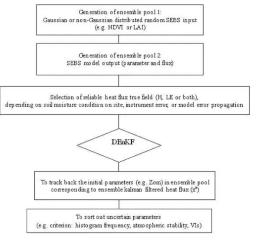
EnKF was used to compensate for the limitations of each model physics with different error structure by merging the model estimates contaminated by aerodynamic rough-ness input errors, but independent from assumption of energy balance closure into the

15

field measurements independent from aerodynamic roughness input errors, but biased by the assumption of energy balance closure. In other words, field measured heat flux estimates were employed as EnKF true field, while hydrological model estimates play a role of relating optimal heat flux to initial parameter input. Brief concept was introduced in Fig. 2. Each of the blocks is explained in following sections.

20

2.1 Field measurement: Bowen Ratio Energy Balance (BREB)

During the experimental period, eddy covariance data were unavailable at the BJ station in Naqu sites in 2006. Instead, the Bowen Ratio Energy Balance (BREB) method was employed, based upon previous validation study with eddy covariance data (van der Velde et al., 2009). BREB estimates heat flux using temperature and

(7)

HESSD

9, 5195–5224, 2012

roughness

J. H. Lee et al.

Title Page

Tables Figures

◭ ◮

Back Close

Full Screen / Esc

Discussion

P

a

per

|

Dis

cussion

P

a

per

|

Discussion

P

a

per

|

Discussio

n

P

a

per

|

vapor pressure gradient as followed.

Bowen ratio(β)=γT1−T2

e₁−e₂ (1-1)

Where, e₁ and e₂ are vapor pressure measurements [kPa] observed at two different levels, while T₁ and T₂ are air temperature [K] measured at the same measurement heights (Z₁/Z₂>4) andγ is psychometric constant [kPa K−1]. This Bowen ratio is

fur-5

ther used to calculate heat flux from surface energy balance.

λE₌Rn−Go

1+β H= β

1+β(Rn−Go) (1-2)

where, G_o₌k_hTskin−Tsl

dz andRn=Ris−Ros+Ril−Rol (1-3) λE is latent heat. H is sensible heat. Soil heat flux (G_o) was determined by thermal

10

conductivity k_h [W mK−1] as a function of soil moisture contents [m3m−3]. z is soil depth, while T_skin is surface temperature. T_sl is soil temperature at depth of 0.05 m. Net radiation (R_n) was combined from inward (R_is), and outward short wave radiation (R_os), inward (R_il), outward (R_ol) long wave radiation, each component of which was measured from radiation sensor (van der Velde et al., 2010).

15

In EnKF, the key to success is the quality of observations used as a true field (a pri-ori). Therefore, to acquire reliable geophysical information representing a characteristic of parameter of interest (here,Z_om), this study rejected most of uncertain and irrelevant measurement data, according to following criteria:

1. Turbulent data withβ below −0.7 were excluded, to forbid latent heat sign error

20

(8)

HESSD

9, 5195–5224, 2012

roughness

J. H. Lee et al.

Title Page

Tables Figures

◭ ◮

Back Close

Full Screen / Esc

Discussion

P

a

per

|

Dis

cussion

P

a

per

|

Discussion

P

a

per

|

Discussio

n

P

a

per

|

2. Heat flux values with incorrect sign were excluded, according to flux and gradient relationship (i.e. latent heat has an opposite sign with respect to specific humid-ity gradient) (Ohmura, 1982). Accordingly, entire data showed negative humidhumid-ity gradient, suggesting positive latent heat (evaporation).

3. To select turbulent characteristics governing aerodynamic momentum roughness,

5

wind measurement data with low velocity (U₂) less than 1 m s−1 and small wind velocity gradient (U₁–U₂<0.3 m s−1) as well as low friction velocity were also ne-glected (Liu and Foken, 2001).

4. In arid region such as Naqu sites, since temperature gradient is required presum-ably more than vapor pressure gradient – which is usually small on dry condition

10

and might be readily contaminated by measurement error, data with low temper-ature gradient (T₂–T₁<0.1 K) were discarded (Yang et al., 2003).

5. Sensible heat fluxes below 10 W m−2 were also excluded to identify convective condition (Yang et al., 2003).

Consequently, this data filtering resulted in sensible heat on free convective turbulent

15

condition ranged above 50 W m−2.

2.2 Model states: Surface Energy Balance System (SEBS)

SEBS was developed to estimate atmospheric fluxes on the large to global scale using satellite earth observation data. As an input, it requires land surface parameters such as canopy height, emissivity, albedo and LAI, and meteorological turbulent data such

20

(9)

HESSD

9, 5195–5224, 2012

roughness

J. H. Lee et al.

Title Page

Tables Figures

◭ ◮

Back Close

Full Screen / Esc

Discussion

P

a

per

|

Dis

cussion

P

a

per

|

Discussion

P

a

per

|

Discussio

n

P

a

per

|

2.2.1 Roughness lengths

Displacement height d₀, aerodynamic Z_om and thermal roughness lengths Z_oh were estimated as followed (Massman, 1997; Su et al., 2001; Su, 2002).

d₀₌h_c

1− 1

2n_ec×(1−exp (−2nec))

(2-1)

5

z_om₌h_c

1−d0

h_c

exp

−ku(hc) u∗

(2-2)

Where, h_c is canopy height estimated as a function of MODIV NDVI. Within-canopy extinction is formulated below.

n_ec₌CdLAI

2

_u₍_h

c)

u∗

2

(2-3)

Here,C_dis drag coefficient of foliage, while LAI is leaf area index. LAI was formulated

10

as a function of MODIS NDVI to be propagated through model. u(h_c)/u∗ was deter-mined from Massman methods (Su et al., 2001). Additionally, by surfaceU∗parameter

K B−1values for mixed canopy and soil, thermal roughness height is related to aerody-namic roughness height (Choudhury and Monteith, 1988).

KB−1₌log

_z

om

z_oh

(2-4)

15

Here, KB−1 is an excess resistance to heat transfer, which is expressed a function of roughness Reynolds number for bare soil surface, while it is estimated from sev-eral parameters of leaf heat transfer coefficient, fractional canopy coverage, and within canopy wind speed profile extinction coefficient for canopy landscape (Su et al.,2005). Accordingly, in this study, if NDVI is under or overestimated, LAI,u(h_c)/u∗, displacement

20

(10)

HESSD

9, 5195–5224, 2012

roughness

J. H. Lee et al.

Title Page

Tables Figures

◭ ◮

Back Close

Full Screen / Esc

Discussion

P

a

per

|

Dis

cussion

P

a

per

|

Discussion

P

a

per

|

Discussio

n

P

a

per

|

2.2.2 Evaporation fraction

The roughness height for heat and momentum (resp. Z_oh and Z_om) determined as above are further used in MOS relationship to estimate sensible heat, and aerodynamic resistance (Su et al., 2002). Sensible heat estimated in this way is further exploited to determine latent heat. In SEBS, latent heat is calculated using evaporative fraction, the

5

ratio of heat fluxes on hypothetical condition (sensible heat on the hypothetical wet/dry condition, and residual latent heat on wet condition) to available energy (Su et al., 2002).

λE_{= Λ}(R_n−G_o) (2-5)

where, evaporative fraction is

10

Λ =ΛrλEwet

R_n−G_o (2-6)

Here, relative evaporation is

Λr=1−

H−H_wet

H_dry−H_wet (2-7)

and

λE_wet₌R_n−G_o−H_wet (2-8)

15

Under the dry condition,H_dry was directly estimated by approximation ofR_n – G_o as-suming latent heat is zero (λE_dry=0). Sensible heat on wet conditionH_wet was formu-lated as followed.

H_wet₌

"

(R_n−G_o)−Cpρair

r_a

(e_sat−e_a)

γ

#

γ

(11)

HESSD

9, 5195–5224, 2012

roughness

J. H. Lee et al.

Title Page

Tables Figures

◭ ◮

Back Close

Full Screen / Esc

Discussion

P

a

per

|

Dis

cussion

P

a

per

|

Discussion

P

a

per

|

Discussio

n

P

a

per

|

Where,r_a₌ 1 kU∗.

ln(z−d0

z_oh )−Ψ

(z−d₀)

L_w + Ψ( z_oh

L_w)

(2-10)

Here,ρ_air is the density of dry air [kg m−3]. C_p is heat capacity [J kgK−1]. e_a is actual vapour pressure at reference height [Pa], whilee_satis saturation vapour pressure at ref-erence height [Pa].r_ais aerodynamic resistance to heat transfer [s m−1].L_wis wet-limit

5

stability length.∆is the rate of change of saturation vapour pressure with temperature, whileγ is the psychometric constant [Pa K−1].

2.3 Implementation of Deterministic Ensemble Kalman Filter (DEnKF)

Deterministic Ensemble Kalman Filter was chosen to match ensemble SEBS heat flux pool with BREB estimates considered as “a priori”. Among other Kalman Fileters,

de-10

terministic ensemble kalman filter was selected because it does not require significant perturbation in observation of latent and sensible heat. In other words, the term of ob-servation perturbation in traditional Kalman filter analysis is set to zero (Sakov et al., 2008; Reichle et al., 2008).

Xa₌Xf₊K(d₊D₋_H_Xf₎₌_Xf₊_K₍d₋_H_Xf_{) where,} _K ₌_Pf_HT_(H_Pf_HT₊_R₎−1 _(3-1) 15

Where,Xa is analysis.Xf is forecast. K is Kalman gain.d _andD _{are respectively the}

observation vector and the synthetic vector of perturbations of observationsd _(here, D₌_{0 in}D_{EnKF), and}_H_{is observation sensitivity matrix as a non-linear operator. The}

objective is to adjust this ensemble analysis (Xa) with anomaly analysis (Aa) deter-mined below.

20

(12)

HESSD

9, 5195–5224, 2012

roughness

J. H. Lee et al.

Title Page

Tables Figures

◭ ◮

Back Close

Full Screen / Esc

Discussion

P

a

per

|

Dis

cussion

P

a

per

|

Discussion

P

a

per

|

Discussio

n

P

a

per

|

ensemble mean (A_i ₌X_i−x, wherex₌_m1Pm

i=1Xi.mis ensemble size.Xi is ensemble

member of model state).

Pa₌ 1 m−1

m

X

i=1

(X_i−x)(X_i−x)T = 1

m−1A

a_AaT _(3-3)

Because of following relationships Aa₌Af₊K(D−HAf)∼₌AfKHAf and D₌0,

PfHTKT₌KHPf, then error covariance in Eq. (3-3) is rearranged as followed (Sakov

5

et al., 2008).

Pa₌Pf−2KHPf₊KHPfHTKT (3-4)

Here, ifKHis negligibly small, analysis can be tuned for quadratic form (KHPfHTKT) by approximation of K ₌1₂K (Whitaker and Hamill, 2002). Accordingly, analysis error covariance and anomaly stated above become:

10

Aa₌Af−1 2KHA

f

(where, Af₌Xf−xf) (3-5)

and

Pa₌(1−KH)Pf₊1

4KHP

f_HT_KT _(3-6)

Now,Xa in Eq. (3-2) can be estimated from analyzed anomaly (Aa) and analysis (xa) achieved from the Kalman filter in Eq. (3-1).

15

The ensemble pool was randomly generated by the assumption of Gaussian distri-bution over NDVI. According to previous study (Moradkhani et al., 2005), Normalized RMSE ratio (NRR: time averaged RMSE over ensemble member averaged RMSE) was used to evaluate and quantify this randomly generated ensemble pool spread. Out of 20 trials (variance ranging from 8 % to 50 %; ensemble size ranging from 20 to 100), a

(13)

HESSD

9, 5195–5224, 2012

roughness

J. H. Lee et al.

Title Page

Tables Figures

◭ ◮

Back Close

Full Screen / Esc

Discussion

P

a

per

|

Dis

cussion

P

a

per

|

Discussion

P

a

per

|

Discussio

n

P

a

per

|

group of 1.05 of NRRH and 1.1 of NRRLE(ensemble size=100, variance=30 %) was in acceptable range (cf. ideal NRR is a unity), and used in this study. Number of ob-servation updated at each assimilation step was equivalent to number of model states. Inflation was set to 1.01.

3 Results

5

3.1 Data assimilation

Only sensible heat was used to identify aerodynamic roughness via EnKF for various reasons. First, ingeneral, it was considered that latent heat in arid area has a degree of uncertainty in measurement. It was suggested that vapour pressure gradient is vulner-able to measurement errors in arid area, since it is much less than temperature gradient

10

on dry condition (Boulet et al., 1997; Jochum et al., 2005; Prueger et al., 2004; Weaver et al., 1992). Second, according to energy budget analysis over the Tibetan Plateau, sensible heat is the dominant energy in ABL (Ma et al., 2009). Additionally, in SEBS, as briefly described in methods 2.2, sensible heat can transfer or amplify its errors to latent heat, because latent heat is calculated from the sensible heat estimated beforehand.

15

Furthermore, Gaussian error propagation through SEBS structure showed that latent heat has higher variance than sensible heat, and is affected by other diverse parameter errors (Marx et al., 2008). For various aerodynamic roughness inputs (with a mean of 0.035 m and standard deviation of 0.016 m, ranging from 0.015 m to 0.055 m), variance of sensible and latent heat propagated by SEBS was estimated

20

as 225 and 331 [W m−2]2. With regard to interference (each parameter was assumed to be independent), latent heat was affected by several other input errors (i.e. LAI,

h_c, Z_oh, d₀) in addition to Z_om, while sensible heat mostly affected by aerodynamic roughness height. In detail, variances for displacement height (20 931 [W m−2]2), thermal roughness height (663 [W m−2]2), canopy height (136 [W m−2]2), and LAI (100

25

(14)

HESSD

9, 5195–5224, 2012

roughness

J. H. Lee et al.

Title Page Abstract Introduction Conclusions References Tables Figures ◭ ◮ ◭ ◮ Back Close

Full Screen / Esc

Printer-friendly Version Interactive Discussion Discussion P a per | Dis cussion P a per | Discussion P a per | Discussio n P a per |

other than aerodynamic roughness was considered significant for sensible heat.

δ_LE2 ₌( ∂LE

∂_Z

om )2δ_Z2

om+(

∂_LE ∂_LAI)

2

δ_LAI2 ₊(∂LE

∂_h

c )2δ_h2

c+(

∂_LE ∂_Z

oh )2δ_Z2

oh+(

∂_LE ∂_d0)

2

δ_d2

0.

δ_H2 ₌( ∂H

∂_Z

om )2δ_Z2

om+(

∂H

∂_h

c )2δ_h2

c.

5

Accordingly, sensible heat was selected to be a more direct indicator for aerodynamic roughness height estimation.

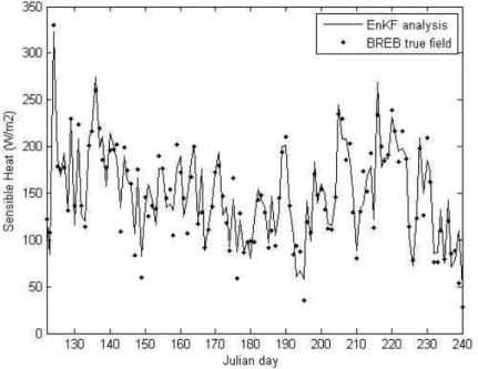
After assimilation, as shown in Fig. 3, RMSE between Ensemble Kalman Filtered sensible heat and initial unperturbed BREB observation successfully improved to 17 W m−2(65 W m−2before data assimilation). Data point holding a large discrepancy

10

with BREB estimates (i.e. to discardx_taif |xa-H_breb|>10 W m−2) was excluded, when it was inversely tracked back to initialZ_omensemble pool in following results 3.2.

3.2 Parameter estimation

Based upon previous Gaussian error propagation analysis that demonstrated relatively more direct and exclusive relationship between sensible heat flux and aerodynamic

15

roughness parameter, the initial aerodynamic roughness input corresponding to sensi-ble heat EnKF analysis were found from ensemsensi-ble pool. This estimate was considered the very initial approximate parameter that offered EnKF final analysis values. During pre-Monsoon period of highly unstable and free convective time that sensible heat is greater than latent heat, only day time unstable sensible heat flux (>150 W m−2) was

20

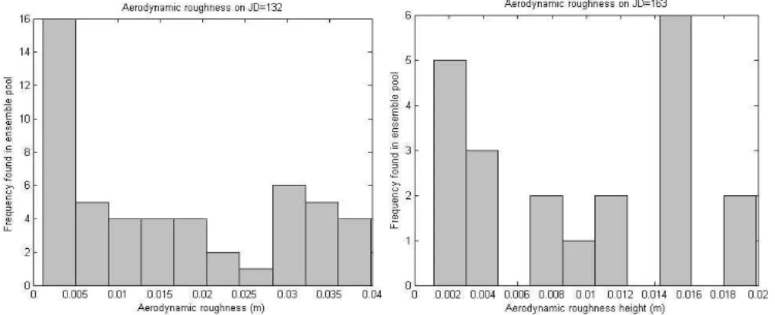
used to estimate aerodynamic roughness (Prueger et al., 2004; de Bruin et al., 1997). Next, since aerodynamic roughness height is usually spread with a high standard de-viation, this study accepted only the values which were the most frequently found in an ensemble pool as in Fig. 4.

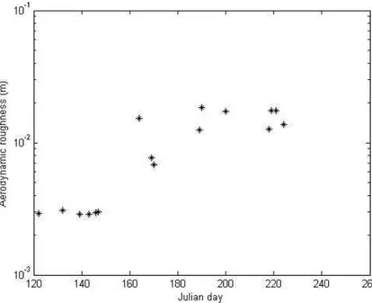
As shown in Fig. 5, resultant aerodynamic roughness height reflected the vegetation

25

(15)

HESSD

9, 5195–5224, 2012

roughness

J. H. Lee et al.

Title Page

Tables Figures

◭ ◮

Back Close

Full Screen / Esc

Discussion

P

a

per

|

Dis

cussion

P

a

per

|

Discussion

P

a

per

|

Discussio

n

P

a

per

|

of 0.0098 m, and standard deviation of 0.0063 m, and range of minimum (0.0029 m) and maximum (0.0186 m). This estimate is consistent with fixed literature value for grasslands (0.01 m: Beljaars et al., 1983), but time-variant. This is also agreeable with previous study carried out with eddy covariance data over the Naqu site (Yang et al., 2003).

5

3.3 Validation

Those aerodynamic roughness height inputs calibrated via EnKF were inserted into original SEBS to examine its influence over heat flux estimation and energy source partitioning.

As shown in Fig. 6, newly estimated aerodynamic and thermal roughness (0.1·Z_om

10

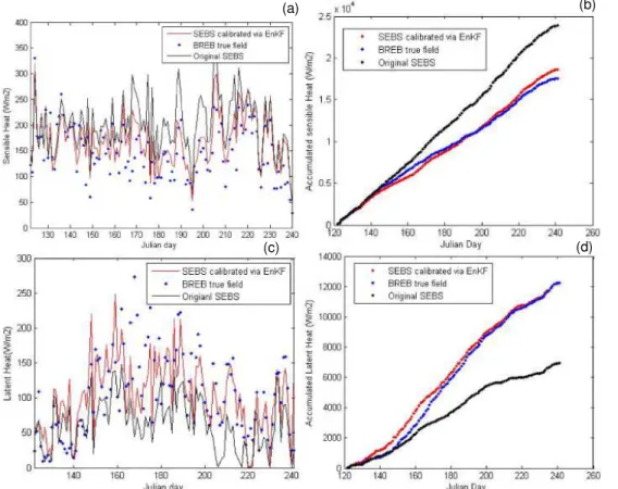
by approximation) reported better RMSE (H: 34 W m−2, LE: 40 W m−2) with unper-turbed BREB heat flux estimates than original SEBS (H: 65 W m−2, LE: 60 W m−2). Here, RMSE (34 W m−2) in sensible heat was found to be slightly higher than the en-semble kalman final analysis reported in Fig. 3 (RMSE: 17 W m−2), because precedent values on previous time step were assigned when no optimal aerodynamic parameter

15

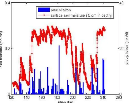
(as Not A Number) was found on certain Julian day. Improvement of heat flux estimates via EnKF was maximized on wet condition. Large discrepancy between original SEBS and EnKF calibration methods was found around Julian day of 180 during the summer Monsoon period. Since soil moisture and precipitation were reported very high during this period as demonstrated in Fig. 7, BREB sensible/latent heat estimates were

con-20

sidered reliable by water balance, suggesting that EnKF calibration approach exhibited intermediate numbers between orginial SEBS and BREB especially during Monsoon period. Thus, it was concluded that heat flux estimation especially during the Monsoon period was improved.

There are various reasons for this higher RMSE in latent heat. First, Gaussian error

25

(16)

HESSD

9, 5195–5224, 2012

roughness

J. H. Lee et al.

Title Page

Tables Figures

◭ ◮

Back Close

Full Screen / Esc

Discussion

P

a

per

|

Dis

cussion

P

a

per

|

Discussion

P

a

per

|

Discussio

n

P

a

per

|

SEBS led to overestimated actual sensible heat (H) by following Eq. (4) below and un-derestimated aerodynamic resistance (r_a) by Eq. (2-10) and wet sensible heat (H_wet) by Eq. (2-9) (Su et al., 2005). Continuously, overestimated sensible heat could further give a rise to underestimated relative evaporation (Λr) by Eq. (2-7), and evaporative fraction (Λ) by Eq. (2-6), and finally latent heat by Eq. (2-5). Here, evaporative fraction

5

itself contains uncertainty because it assumes wet and dry condition.

T_sur−T_air₌ H kU∗_pC

p

ln(z−d0

z_oh )−Ψ( z−d₀

L )+ Ψ( z_oh

L )

(4)

Where,T_surandT_air are potential temperature for land surface and air at the reference height. ψ is stability correction function for sensible heat transfer, and L is Obukhov length (Su, 2005).

10

As shown in Fig. 6, Naqu site experienced seasonal variations in heat flux, alter-ing the Bowen ratio over time. Vertical gradients of temperature and humidity in ABL also showed a dramatic change in the middle June around onsets of Monsoon period (data not shown). During the Monsoon period with heavy precipitation events (Fig. 7), latent heat increased with a decrease in Bowen ratio (approximate mean: 2.3), while

15

it showed higher Bowen ratios (approximate mean: 17 before Monsoon, and 4.4 after Monsoon) and sensible heat before/after Monsoon.

From comparison in accumulated heat flux (Fig. 6b and d), it was also found that ac-cumulated latent heat flux is less than sensible heat, suggesting the dominant energy source at this region is sensible heat even during Monsoon. This also confirmed that the

20

assumption used – a selection of sensible heat in data assimilation – was reasonable. It was thought that high sensible heat (above 150 W m−2) developed convective activities in atmospheric boundary layer (ABL) before Monsoon period, resulting in precipita-tion as a feedback during summer Monsoon (Ma et al., 2009; Wen et al., 2010). This Monsoon precipitation further elevated surface soil moisture (reached up to 0.3 m3m−3

25

(17)

HESSD

9, 5195–5224, 2012

roughness

J. H. Lee et al.

Title Page

Tables Figures

◭ ◮

Back Close

Full Screen / Esc

Discussion

P

a

per

|

Dis

cussion

P

a

per

|

Discussion

P

a

per

|

Discussio

n

P

a

per

|

and latent heat, but suppressed sensible heat, suggesting a high correlation of surface soil moisture with latent heat patterns (Li et al., 2010).

Another validation was carried out with eddy covariance data over maize field at Lan-driano station, in Italy during vegetation proliferation period (the beginning of July to the middle of October) where, atmospheric condition is mostly unstable, and soil moisture

5

is moderately high (0.25∼0.35). Unlike previous BREB data in arid condition, it was considered that both latent and sensible heat fluxes made a contribution to uncertainty (to the same extent, 15∼20 % for both, Chavez et al., 2005) since latent heat plays a dominant role in energy budget (daily average sensible heat observation by eddy co-variance data during experimental period: 10 W m−2) under wet condition. Accordingly,

10

both heat fluxes were assimilated by EnKF. For a comparison, aerodynamic roughness formulated as a function of LAI and drag force showed a mean of 0.32 m (Olioso et al., 2002). One determined by a traditional wind profile method including atmospheric sta-bility correction on both neutral and non-neutral condition reported a mean of 0.18 m (Ma et al., 2008). Aerodynamic roughness inversely tracked by EnKF illustrated an

15

intermediate value of 0.25 m as a mean and 0.04 m as standard deviation.

4 Conclusions

In heat flux estimation, aerodynamic roughness is a major uncertain input. Unlike other parameters such as pressure, land surface temperature or surface soil moisture, this parameter can be indirectly estimated using eddy covariance data, which covers only

20

limited fetch size on a local scale. However, due to measurement errors and land surface-atmospheric conditions not satisfying MOS assumptions, data inclined to be scattered with high standard variations. In a larger scale, a method using remotely sensed vegetation index can be employed. However, this still requires drag force in-put obtained from eddy covariance data, and also can be applied to limited

vegeta-25

(18)

HESSD

9, 5195–5224, 2012

roughness

J. H. Lee et al.

Title Page

Tables Figures

◭ ◮

Back Close

Full Screen / Esc

Discussion

P

a

per

|

Dis

cussion

P

a

per

|

Discussion

P

a

per

|

Discussio

n

P

a

per

|

a complicated procedure requiring the accuracy of several other related parameters involved in MOS theory.

Thus, this study demonstrated a simpler operational framework to retrieve a pa-rameter of aerodynamic roughness via EnKF that affords non-linearity. This method demands only single or two heat flux parameters, which were elected by model

er-5

ror structure analysis. This study successfully adjusted the heat flux outputs over or underestimated by original SEBS, allowing more reliable interpretation for energy par-titioning and water cycle. At the onset of Monsoon, this improvement was remarkable. Main energy source in Naqu site was still sensible heat even during Monsoon period, and latent heat was minor before/after Monsoon precipitation. Aerodynamic roughness

10

estimated in this study was time-variant, reflecting vegetation effects, and independent from remotely sensed VI saturation problem. It was demonstrated that this approach can be applied to the local field where eddy covariance data are not available. This may replace existing wind profile or vegetation index approach as an alternative. Fu-ture work will include some scale issues: the application of this approach to a larger

15

scale with heterogeneity. The forest area where it is difficult to identify the vertical char-acteristics with remotely sensed VIs is also an interest. Effect of observation update regime – e.g. in case of satellite data with low temporal frequencies – can be explored in future data assimilation study.

Acknowledgements. We give special thanks to Pavel Sakov who provided ensemble Kalman 20

Filter algorithm and van der Velde and Zeyong Hu for meteorological data over Naqu site, as well as Giovanni Ravazzani who supported this study in the framework of the “ACQWA EU/FP7” project (grant number 212250) “Assessing Climate impacts on the Quantity and quality of WAter”. We are grateful to the reviewers and editors for constructive comments to improve this manuscript.

(19)

HESSD

9, 5195–5224, 2012

roughness

J. H. Lee et al.

Title Page

Tables Figures

◭ ◮

Back Close

Full Screen / Esc

Discussion

P

a

per

|

Dis

cussion

P

a

per

|

Discussion

P

a

per

|

Discussio

n

P

a

per

|

References

Beljaars, A. C. M., Schotanus, P., and Nieuwstadt, F. T. M.: Surface layer similarity under nonuni-form fetch conditions, J. Clim. Appl. Meteorol., 22, 1800–1810, 1983.

Boulet, G. , Braud, I., and Vauclin. M.: Study of the mechanisms of evaporation under arid conditions using a detailed model of the soil-atmosphere continuum, J. Hydrol., 193, 114– 5

141, 1997.

Chavez, J. L., Neale, C. M. U., Hipps, L. E., Prueger, J. H., and Kustas, W. P.: Comparing aircraft-based remotely sensed energy balance fluxes with eddy covariance tower data using heat flux source area functions, J. Hydromet., AMS, 66, 923–940, 2005.

Chen, R. K. and Yang, C. M.: Determining the Optimal Timing for Using LAI and NDVI to Predict 10

Rice Yield, Journal of Photogrammetry and Remote Sensing, 103, 239–254, 2005.

Choi, T., Kim, J., Lee, H., Hong, J., Asanuma, J., Ishikawa, H., Gao, Z., Wang, J., and Koike., T.: Turbulent exchange of heat, water vapor, and momentum over a Tibetan prairie by eddy covariance and flux variance measurements, J. Geophys. Res., 109, D21106, doi:10.1029/2004JD004767, 2004.

15

Choudhury, B. J. and Monteith, J. L.: A four-layer model for the heat budget of homogeneous land surfaces, Q. J. Roy. Meteorol. Soc., 114, 373–398, 1988.

De Bruin, H. A. R. and Verhoef, A.: A new method to determine the zero-plane displacement, Bound.-Lay. Meteorol., 82, 159–164, 1997.

Evensen, G.: Sampling strategies and square root analysis schemes for the EnKF, Ocean Dy-20

nam. 54, 539–560, 2004.

Foken, T. H. and Wichura, B.: Tools for quality assessment of surface-based flux measure-ments, Agr. Forest. Meteorol., 78, 83–105, 1996.

Jochum, M. A. O., de Bruin, H. A. R., Holtslag, A. A. M., and Belmonte, A. C.: Area-Averaged Surface Fluxes in a Semiarid Region with Partly Irrigated Land Lessons Learned from 25

EFEDA, J. Appl. Meteorol. Climatol., 45, 856–874, 2006.

Kohsiek, W., de Bruin, H. A. R., The, H., and van den Hurk, B.: Estimation of the sensible heat flux of a semi-arid area using surface radiative temperature measurements, Bound.-Lay. Meteorol., 63, 213–230, 1993.

Li, F., Crow, W. T., and Kustas, W. P.: Towards the estimation root-zone soil moisture via the si-30

(20)

HESSD

9, 5195–5224, 2012

roughness

J. H. Lee et al.

Title Page

Tables Figures

◭ ◮

Back Close

Full Screen / Esc

Discussion

P

a

per

|

Dis

cussion

P

a

per

|

Discussion

P

a

per

|

Discussio

n

P

a

per

|

Liu, H. and Foken, T.: A modified Bowen ratio method to determine sensible and latent heat fluxes, Meteorologische Z., 10, 71–80, 2001.

Ma, J. and Daggupaty, S. M.: Using All Observed Information in a Variational Approach to MeasuringZ_omandZ_0t, Am. Meteorol. Soc., 1391–1401, 1999.

Ma, Y., Tsukamoto, O., Wang, J., Ishikawa, H., and Tamagawa, I.: Analysis of aerodynamic and 5

thermodynamic parameters over the grassy marshland surface of Tibetan Plateau, Prog. Nat. Sci., 121, 36–40, 2002.

Ma, Y., Fan, S., Ishikawa, H., Tsukamoto, O., Yao, T., Koike, T., Zuo, H., Hu, Z., and Su, Z.: Di-urnal and inter-monthly variation of land surface heat fluxes over the central Tibetan Plateau area, Theor. Appl. Climatol., 80, 259–273, 2005.

10

Ma, Y., Menenti, M., Feddes, R., and Wang, J.: Analysis of the land surface heterogeneity and its impact on atmospheric variables and aerodynamic and thermodynamic roughness lengths, J. Geophys. Res., 113, D08113, doi:10.1029/2007JD009124, 2008.

Ma, Y., Wang, Y., Wu, R., Hu, Z., Yang, K., Li, M., Ma, W., Zhong, L., Sun, F., Chen, X., Zhu, Z., Wang, S., and Ishikawa, H.: Recent advances on the study of atmosphere-land 15

interaction observations on the Tibetan Plateau, Hydrol. Earth Syst. Sci., 13, 1103–1111, doi:10.5194/hess-13-1103-2009, 2009.

Margulis, S. A., McLaughlin, D., Entekhabi, D., and Dunne. S.: Land data assimilation and estimation of soil moisture using measurements from the Southern Great Plains 1997 Field Experiment, Water Resour. Res., 38, 1299, doi:10.1029/2001WR001114, 2002.

20

Marx., A., Kunstmann, H., Schuttemeyer, D., and Moene, A. F.: Uncertainty analysis for satellite derived sensible heat fluxes and scintillometer measurements over Savannah environment and comparison to mesoscale meteorological simulation results, Agr. Forest Meteorol., 148, 656–667, 2008.

Massman, W. J.: An analytical one-dimensional model of momentum transfer by vegetation of 25

arbitrary structure, Bound.-Lay. Meteorol., 83, 407–421, 1997.

Montaldo, N., Albertson, J. D., Mancini, M., and Kiely, G.: Robust simulation of root-zone soil moisture with assimilation of surface soil moisture data, Water Resour. Res., 37, 2889–900, 2001.

Montaldo, N., Albertson, J. D., and Mancini, M.: Dynamic Calibration with an Ensemble Kalman 30

(21)

HESSD

9, 5195–5224, 2012

roughness

J. H. Lee et al.

Title Page

Tables Figures

◭ ◮

Back Close

Full Screen / Esc

Discussion

P

a

per

|

Dis

cussion

P

a

per

|

Discussion

P

a

per

|

Discussio

n

P

a

per

|

Moradkhani, H., Sorooshian, S., Gupta, H. V., and Houser, P. R.: Dual state–parameter estima-tion of hydrological models using ensemble Kalman filter, Adv. Water Resour., 28, 135–147, 2005.

Nobel., P. S.: Physicochemical and environmental plant physiology, San Diego, Academic Press, 474, 1999.

5

Ohmura, A.: Objective criteria for rejecting data for Bowen ratio flux calculations, Am. Meteorol. Soc., 21, 595–598, 1982.

Olioso, A., Jacob, F., Hadjar, D., Lecharpentier, P., and Hasager, C. B.: Spatial distribution of evapotranspiration and aerodynamic roughness from optical remote sensing, in: Proceed-ings of the International Workshop on Landscape Heterogeneity and Aerodynamic Rough-10

ness: Modelling and Remote Sensing Perspectives, edited by: Debie, H. and de Ridder K., (19–26) 12 October 2001, Antwerp, Belgique, VITO, 2002.

Perez, P. J., Castellvi, F., Iba ˜nez, M., and Rosell, J. I.: Assessment of reliability of Bowen ratio method for partitioning fluxes, Agr. Forest Meteorol., 97, 141–150, 1999.

Prueger, J. H., Kustat, W., Hipps, L. E., and Hatfield. J. L.: Aerodynamic parameters and sensi-15

ble heat flux estimates for a semi-arid ecosystem, J. Arid Environ., 57, 87–100, 2004. Reichle, R. H., McLaughlin, D. H., and Entekhabi, D.: Hydrologic Data Assimilation with

the Ensemble Kalman Filter, Mon. Weather. Rev., 130, 103–114, doi:10.1175/1520-0493(2002)130¡0103:HDAWTE¿2.0.CO;2, 2002.

Reichle, H. R.: Data assimilation methods in the Earth sciences, Adv. Water Resour., 31, 1411– 20

1418, 2008.

Richter, K. and Timmermans, W. J.: Physically based retrieval of crop characteristics for im-proved water use estimates, Hydrol. Earth Syst. Sci., 13, 663–674, doi:10.5194/hess-13-663-2009, 2009.

Sakov, P. and Oke, P. R.: A deterministic formulation of the ensemble kalman filter:an alternative 25

to ensemble sqaure root filters, Tellus, 60A, 361–371, 2008.

Scanlon, T. M., Albertson, J. D., and Kustas, W. P.: Scale effects in estimating large eddy-driven sensible heat fluxes over heterogenous terrain. Remote sensing and Hydrology 2000 Proceedings of a symposium held at Santa Fe, USA, April 2000, IAHS Publ. no. 267, 2001. Su, Z.: The Surface Energy Balance System (SEBS) for estimation of turbulent heat fluxes, 30

Hydrol. Earth Syst. Sci., 6, 85–100, doi:10.5194/hess-6-85-2002, 2002.

(22)

HESSD

9, 5195–5224, 2012

roughness

J. H. Lee et al.

Title Page

Tables Figures

◭ ◮

Back Close

Full Screen / Esc

Discussion

P

a

per

|

Dis

cussion

P

a

per

|

Discussion

P

a

per

|

Discussio

n

P

a

per

|

Su, Z., Schmugge, T., Kustas, W. P., and Massman, W. J.: An evaluation of two models for estimation of the roughness height for heat transfer between the land surface and the atmo-sphere, J. Appl. Meteorol., 40, 1933–1951, 2001.

Sun, F., Ma, Y., Ma, W., and Li, M.: One observational study on atmospheric boundary layer structure in Mt. Qomolangma region, Plateau Meteorology, 256, 1014–1019, 2006.

5

Sun, F., Ma, Y., Li, M., Ma, W., Tian, H., and Metzge, S.: Boundary layer effects above a Himalayan valley near Mount Everest, Geophys. Res. Lett., 34, L08808, doi:10.1029/2007GL029484, 2007.

Sun, J.: Diurnal variations of thermal roughness height over a grassland, Bound.-Lay. Meteorol., 92, 407–427, 1999.

10

Timmermans, J., van der Tol, C., Verhoef, A., Verhoef, W., Su, Z., van Helvoirt, M., and Wang, L.: Quantifying the uncertainty in estimates of surface- atmosphere fluxes through joint eval-uation of the SEBS and SCOPE models, Hydrol. Earth Syst. Sci. Discuss., 8, 2861–2893, doi:10.5194/hessd-8-2861-2011, 2011.

Tsuanga, B. J., Tsaia, J. L., Lina, M. D., and Chen, C. L.: Determining aerodynamic roughness 15

using tethersonde and heat flux measurements in an urban area over a complex terrain, Atmos. Environ., 37, 1993–2003, 2003.

van der Tol, C., van der Tol, S., Verhoef, A., Su, B., Timmermans, J., Houldcroft, C., and Gieske, A.: A Bayesian approach to estimate sensible and latent heat over vegetated land surface, Hydrol. Earth Syst. Sci., 13, 749–758, doi:10.5194/hess-13-749-2009, 2009.

20

van der Velde, R.: Soil moisture remote sensing using active microwaves and land surface modeling, Ph.D. thesis, 2010.

van der Velde, R., Su, Z., Ek, M., Rodell, M., and Ma, Y.: Influence of thermodynamic soil and vegetation parameterizations on the simulation of soil temperature states and surface fluxes by the Noah LSM over a Tibetan plateau site, Hydrol. Earth Syst. Sci., 13, 759–777, 25

doi:10.5194/hess-13-759-2009, 2009.

Weaver, H. L.: Temperature and humidity flux-variance relations determined by one-dimensional eddy correlation, Bound.-Lay. Meteorol., 53, 77–91, 1990.

Wen, L., Cui, P., Li, Y., Wang, C., Liu, Y., Chen, N., and Su, F.: The influence of sensible heat on Monsoon precipitation in central and eastern Tibet, Meteorol. Appl., 17, 452–462, 2010. 30

(23)

HESSD

9, 5195–5224, 2012

roughness

J. H. Lee et al.

Title Page

Tables Figures

◭ ◮

Back Close

Full Screen / Esc

Discussion

P

a

per

|

Dis

cussion

P

a

per

|

Discussion

P

a

per

|

Discussio

n

P

a

per

|

Wieringa, J.: Updating the Davenport roughness classification, J. Wind Eng. Ind. Aerodyn. 41– 44, 357–368, 1992.

Yang, K., Koike, T., and Yang, D.: Surface flux parameterization in the Tibetan plateau, Bound.-Lay. Meteorol., 116, 245–262, 2003.

Yang, K., Koike, T., Ishikawa, H., Kim, J., and Li, X.: Turbulent flux transfer over bare-soil 5

surfaces: Characteristics and parameterization, J. Appl. Meteorol. Climatol., 47, 276–290, doi:10.1175/2007JAMC1547.1, 2008.

Yang, P., Chen, Z., Zhou, Q., Zha, Y., Wu, W., and Shibasaki, R.: Comparisons of MODIS LAI products and LAI estimates derived from Landsat TM, Geoscience and Remote Sensing Symposium, IEEE International Conference on 31 July 2006–4 August 2006, 2681–2684, 10

doi:10.1109/IGARSS.2006.692, 2006.

(24)

HESSD

9, 5195–5224, 2012

roughness

J. H. Lee et al.

Title Page

Tables Figures

◭ ◮

Back Close

Full Screen / Esc

Discussion

P

a

per

|

Dis

cussion

P

a

per

|

Discussion

P

a

per

|

Discussio

n

P

a

per

|

Fig. 1.Bias in aerodynamic roughness height estimation over short grassland: from AROME

(25)

HESSD

9, 5195–5224, 2012

roughness

J. H. Lee et al.

Title Page

Tables Figures

◭ ◮

Back Close

Full Screen / Esc

Discussion

P

a

per

|

Dis

cussion

P

a

per

|

Discussion

P

a

per

|

Discussio

n

P

a

per

|

(26)

HESSD

9, 5195–5224, 2012

roughness

J. H. Lee et al.

Title Page

Tables Figures

◭ ◮

Back Close

Full Screen / Esc

Discussion

P

a

per

|

Dis

cussion

P

a

per

|

Discussion

P

a

per

|

Discussio

n

P

a

per

|

(27)

HESSD

9, 5195–5224, 2012

roughness

J. H. Lee et al.

Title Page

Tables Figures

◭ ◮

Back Close

Full Screen / Esc

Discussion

P

a

per

|

Dis

cussion

P

a

per

|

Discussion

P

a

per

|

Discussio

n

P

a

per

|

(28)

HESSD

9, 5195–5224, 2012

roughness

J. H. Lee et al.

Title Page

Tables Figures

◭ ◮

Back Close

Full Screen / Esc

Discussion

P

a

per

|

Dis

cussion

P

a

per

|

Discussion

P

a

per

|

Discussio

n

P

a

per

|

(29)

HESSD

9, 5195–5224, 2012

roughness

J. H. Lee et al.

Title Page

Tables Figures

◭ ◮

Back Close

Full Screen / Esc

Discussion

P

a

per

|

Dis

cussion

P

a

per

|

Discussion

P

a

per

|

Discussio

n

P

a

per

|

Fig. 6.Comparison in heat flux estimates:(a) sensible heat,(b) accumulated sensible heat,

(30)

HESSD

9, 5195–5224, 2012

roughness

J. H. Lee et al.

Title Page

Tables Figures

◭ ◮

Back Close

Full Screen / Esc

Discussion

P

a

per

|

Dis

cussion

P

a

per

|

Discussion

P

a

per

|

Discussio

n

P

a

per

|

Fig. 7.Seasonal change in surface soil moisture measured at 5 cm in depth and rainfall