Model Selection in Historical Research Using
Approximate Bayesian Computation
Xavier Rubio-Campillo*
Computer Applications in Science & Engineering department, Barcelona Supercomputing Centre, Barcelona, Spain
Abstract
Formal Models and History
Computational models are increasingly being used to study historical dynamics. This new trend, which could be named Model-Based History, makes use of recently published data-sets and innovative quantitative methods to improve our understanding of past societies based on their written sources. The extensive use of formal models allows historians to re-evaluate hypotheses formulated decades ago and still subject to debate due to the lack of an adequate quantitative framework. The initiative has the potential to transform the disci-pline if it solves the challenges posed by the study of historical dynamics. These difficulties are based on the complexities of modelling social interaction, and the methodological issues raised by the evaluation of formal models against data with low sample size, high variance and strong fragmentation.
Case Study
This work examines an alternate approach to this evaluation based on a Bayesian-inspired model selection method. The validity of the classical Lanchester’s laws of combat is exam-ined against a dataset comprising over a thousand battles spanning 300 years. Four varia-tions of the basic equavaria-tions are discussed, including the three most common formulavaria-tions (linear, squared, and logarithmic) and a new variant introducing fatigue. Approximate Bayesian Computation is then used to infer both parameter values and model selection via Bayes Factors.
Impact
Results indicate decisive evidence favouring the new fatigue model. The interpretation of both parameter estimations and model selection provides new insights into the factors guid-ing the evolution of warfare. At a methodological level, the case study shows how model selection methods can be used to guide historical research through the comparison between existing hypotheses and empirical evidence.
a11111
OPEN ACCESS
Citation:Rubio-Campillo X (2016) Model Selection in Historical Research Using Approximate Bayesian Computation. PLoS ONE 11(1): e0146491. doi:10.1371/journal.pone.0146491
Editor:John P. Hart, New York State Museum, UNITED STATES
Received:May 25, 2015
Accepted:December 17, 2015
Published:January 5, 2016
Copyright:© 2016 Xavier Rubio-Campillo. This is an open access article distributed under the terms of the Creative Commons Attribution License, which permits unrestricted use, distribution, and reproduction in any medium, provided the original author and source are credited.
Data Availability Statement:Dataset is distributed under the terms of a Creative Commons Attribution-ShareAlike 4.0 International License and accessible athttps://github.com/xrubio/lanchester
Funding:Funding for this work was provided by the SimulPast Consolider Ingenio project (CSD2010-00034) of the former Ministry for Science and Innovation of the Spanish Government and the European Research Council Advanced Grant EPNet (340828).
Introduction
The discipline of History presents its ideas as descriptive models expressed in natural language. Historians use the flexibility of this communication system to explain the complexity and diversity of human societies though their written records. The approach is different than the majority of scientific disciplines, which formulate their theories in formal languages such as mathematics. Formal languages are not as flexible as natural languages, but they are much bet-ter defining concepts and relations without ambiguities [1]. Hypotheses defined in formal lan-guage can then be falsified against empirical evidence, and quantitative methods can then be applied to compare predictions generated by a theory to observed patterns. As a consequence, an old theory can be replace by a new one when it has superior explanatory power.
This evaluation of ideas does not happen in History. Quantitative methods cannot be used to falsify descriptive models or perform cross-temporal and cross-spatial comparison. These inabilities are central to the current methodological debates of the discipline [2–6]. There is a clear desire to identify both the common trajectories and the observed differences between case studies with diverse spatiotemporal coordinates. However, it is unclear how this could be achieved using the common methods of the discipline.
A possible approach to tackle this challenge is to shift the discipline from descriptive to for-mal models [7]. This innovation could allow historians to know under what extent a working hypothesis explains a historical dynamic by quantifying the distance between the predictions of a model and the patterns observed in the evidence. This new approach has clear benefits, but it is not an easy task as it requires a) formal models, b) quantified datasets and c) methods to compare both components.
These debates are intrinsically linked with the increasing number of available databases and historical research using formal models [8–10]. The rise of what we could define as Model-Based Historyis changing the way researchers study historical trajectories [2]. To date, this new approach to the past has been focused on three main topics: trade networks [11], sociocul-tural evolution [7] and warfare [12–14]). The increase in the number of works is diversifying the topics examined byModel-Based History, and now it includes fields such as knowledge exchange [15] or the evolution of religion [16].
Quantitative comparison between models and observations is one of the advantages of this new approach. The most common statistical framework to perform this evaluation is Null Hypothesis Significance Testing. First, the problem to solve is defined as a clear research ques-tion and a working hypothesisH1. This hypothesis is a possible answer which could be falsified by existing evidence. The explanation provided byH1 will then compete against a null hypoth-esisH0.H0 is an alternative that does not take into accountH1.H1 is translated into a formal model, usually a computer simulation of the dynamics encapsulated in the hypothesis. Model-Based Historyoften prefers bottom-up techniques such as Agent-Based Models [17] or com-plex network analysis [18]. Classical equation-based models are also applied, but these innova-tive approaches seem better suited to the type of social processes examined by the discipline. The created model defines the system at a small-scale level (e.g. individual or groups), and it evolves through the interaction between these entities. The emergence of distinctive large-scale patterns generated by this set of interactions is then compared to empirical data. If the proba-bility of getting the observed patterns withoutH1 is less than a given confidence interval (i.e. thep-value) we can rejectH0, thus acceptingH1.
increasing popularity due to the current debates on the use of statistics analysis for scientific research [19–23]. It is worth mentioning that neither method seems better than the other one, and the choice will depend on the aim of the research: Null Hypothesis Significance Testing aims to know if the observed process could be explained without the working hypothesis, while model selection aims to choose which hypothesis is better at matching evidence.
The model selection approach provides a set of new methods to evaluate models. Most of them quantify the loss of information from each model to the evidence using information crite-ria [24]. Two of the most widely used methods are Akaike Information Criterion and Bayesian Information Criterion. Both of them fit the different models to the observed patterns using maximum likelihood methods, and then they calculate an index of information loss (i.e. low values indicate better models).
A different solution is to use the Bayesian statistical framework. It is based on the idea that the knowledge of a given system with uncertainty can be gradually updated through new evi-dence. The process is achieved by computing the probability that a given hypothesis is correct, considering both existing knowledge and new data. The main advantage of this approach is that it seems better fitted to evaluate competing models under high levels of uncertainty and equifinality [25]. Despite its interest, scientific research did not start using the Bayesian frame-work until recent years, even if it was formulated 200 years ago [26]. The delay on the adoption was mainly caused by the mathematical complexities of applying Bayesian statistics to non-trivial problems. The development of new computational methods such as Markov Chain Monte-Carlo and Approximate Bayesian Computation (ABC) has mainly solved this limita-tion, thus explaining the current success of Bayesian inference.
Historians constantly deal with competing explanations of uncertain datasets, so it seems that Bayesian model selection can be useful to the discipline. This potential can also be inferred from the fact that other historical disciplines such as biology and archaeology are part of this Bayesian renaissance. Biology is particularly active in using these methods in fields such as population genetics and ecology [27,28]. Archaeology traditionally limited Bayesian inference to C14 dates [29], but model selection techniques are becoming popular beyond this applica-tion [30–33]. These examples suggest that Bayesian model selection can be applied to History, considering the similarities between the three disciplines. First, all these fields study temporal trajectories using data with high levels of uncertainty. Second, the analysis of these datasets implies that they need to evaluate the plausibility of multiple competing hypotheses. Finally, all of them want to identify patterns generated as an aggregate of individual behaviour. As a con-sequence, it seems clear that Bayesian model selection would have significant utility for historians.
This paper presents the use of Bayesian inference to perform model selection in historical research. The utility of a Bayesian-inspired computational method known as Approximate Bayesian Computation is discussed. The use of ABC is then illustrated with a classical example of formal model used in History: the classical Lanchester’s laws of warfare. Next section pres-ents the case study, the model selection framework and the competing models. Third section shows the results of the method, both in terms of model selection and parameter estimation. The text then interprets these results and concludes with an evaluation of the approach in the context ofModel-Based History.
Materials and Methods
Case study: the evolution of combat
officers on managing armies and fighting the enemy. These practices had a major impulse dur-ing Second World War with the creation ofOperations Research. This new research field focused on developing formal models able to help commanders on decision-making [34]. The introduction of the first computers expedited the use of these quantitative methods during the Cold War, establishing them as a standard procedure for training and planning. In contrast, History is only now incorporating some of these techniques to the study of past conflicts [35]. Boardgames, mathematical models and computer simulations are proving their utility in the task of studying warfare understood as an unfortunate part of human culture [36].
The theoretical model formulated by F.W. Lanchester in 1916 is one of the most popular mathematical formulations used in the field [37]. Lanchester aimed to design the laws predict-ing the casualties of two enemy forces engaged in land battle. He proposed a system of coupled differential equations where casualties were dependent on two factors: a) force size and b) fighting value. The first factor takes into account the importance of sheer numbers on the out-come of military conflict, while the second factor encapsulates qualitative differences between individual fighting skills (e.g. morale, training, technology, etc.). Two models were initially pro-posed: thelinear lawand thesquare law. Thelinear lawaimed to capture the dynamics of ancient battles, where the supremacy of hand-to-hand combat meant that each soldier could only attack an opponent at a given moment. The equations defining the rate of casualties in a battle between armies Blue and Red are defined inEq 1:
dB
dt ¼ rBR
dR
dt ¼ bRB ð1Þ
withB, Ras the size of the forces andr, bas theirfighting value. The rate of casualties is propor-tional to both sizes, so even highly disproportionate odds would cause similar casualties to both opponents.
Thesquare lawmodels warfare after the introduction of gunpowder-based weapons. This technological innovation increased the range, thus allowing each soldier to attack multiple ene-mies. Thesquared lawmodels the casualties of a force as the enemy’s force size multiplied by the fighting value of its individuals, as seen inEq 2:
dB
dt ¼ rR
dR
dt ¼ bB ð2Þ
The Lanchester’s laws generated a large amount of interest during the Cold War [38–42]. The debate was centred on the actual predictive power of the laws, and it included the formula-tion of alternate proposals such as the popularlogarithmicmodel. It suggested that the casual-ties suffered by a force are not dependant on the enemy’s size, but on its own size as defined in
Eq 3[40]:
dB
dt ¼ rB
dB
dt ¼ bR ð3Þ
Several works discussed the validity of the laws [42,43]. Other contributions extended the original framework introducing concepts such as spatial structure or system dynamics [44,45]. The utility of the model was also expanded beyond its initial purpose, and has been successfully applied to study competition dynamics in ecology [46–48], evolutionary biology [49] or eco-nomics [50].
that the logarithmic model has higher explanatory power than the two classical models. How-ever, the coarse-grained results assumed that this power remained constant during the whole period, thus not examining the validity of the models for the different phases of warfare. Simi-lar works used Bayesian inference to evaluate the Lanchester’s laws in specific scenarios. They included biological case studies [48], daily casualties during Inchon-Seoul campaign in 1950 [52] or attrition during the battle of the Ardennes in 1944 [53,54].
All these results suggests that the Lanchester’s laws are useful to understand if casualties are more influenced by quantitative or qualitative factors. Some authors suggested that the models should introduce dynamic parameters such as variable fighting values or fatigue [44]. However, as some of these works highlights, a pure Bayesian framework could hardly cope with the mathematical difficulties added by this new complexity.
The dataset. The dataset used in this study is based on Allen’s list of battles, originally compiled in a previous work [55]. The introduction of weapons with longer ranges over 300 years should be reflected in a gradual increase in the validity of thesquaredmodel over the lin-earmodel. In order to test this idea the span has been divided in four periods, based on prior opinions of decisive transitions in the evolution of warfare [56]:
1. Pike and Musket (1620–1701). The first period was characterised by deep formations of
sol-diers (i.e.terciosand regiments) armed with muskets and pikes.
2. Linear warfare (1702–1792). The War of the Spanish Succession (1702–1714) saw a shift in
battle tactics and technological innovations. Armies were deployed in thin formations exclu-sively armed with muskets, while pikes were substituted by bayonets.
3. Napoleonic Wars (1793–1860). The French Revolution forced another major transition in
warfare, which was mainly adopted during the Napoleonic wars. The new concept ofcitizen armies allowed the states to increase the size of their forces up to the limits imposed by pre-industrial logistics.
4. American Civil War (1861–1905). The impact of industry development became explicit on
the battlefield during the American Civil War. The size of armies and the lethality of their weapons steadily increased until fully industrialised armies were deployed in the Russo-Jap-anese War. This conflict was the prelude of what would be seen during the two world wars.
Exploratory Data Analysis has been used to identify structural patterns in the dataset. A time series of the number of battles can be seen inFig 1, while size and casualty ratios are depicted inFig 2. These visualisations shows how the dataset has relative small sample size and high variance. These are common properties seen in historical data. The figures suggest that the number of battles remained constant during the 300 years with the exception of the Napo-leonic Wars. At the same time, the gradual increase on average army size seems linked to a decrease on casualty ratios.
The model selection framework
posterior distribution) is then computed following Bayes’rule:
PðyjDÞ ¼PðDjyÞ PðyÞ
PðDÞ
beingθthe considered value andDthe observed data. This can be translated as (following [57]):
posterior¼likelihoodprior
evidence
A barrier to the adoption of Bayesian inference is the difficulty to derive likelihood functions when the examined model is not a standard statistical distribution. This constraint limits the use of the framework for computer simulations encapsulating complex dynamics such as the ones explored inModel-Based History. A major breakthrough to this issue is the recent devel-opment of ABC [58,59].
ABC comprises a family of computationally-intensive algorithms able to approximate pos-terior distributions without using likelihood functions. These methods identify the regions of the prior space producing the closest results to the evidence. This capability of extending the Bayesian framework to any computer simulation has exponentially increased the popularity of ABC during the last decade, including the other historical disciplines: biology [60–63], and archaeology [31,33,64,65]).
The analysis performed in this work implements the simplest ABC method: the rejection algorithm [66]. It is not the most efficient ABC method (see [67,68] for alternatives), but its
Fig 1. Number of battles by decade.The three identified transitions correlate with periods of intensive warfare.
simplicity and lack of assumptions makes it perfect for illustrative purposes. It is defined as follows:
1. Initialise parameters sampling the prior distributions
2. Run the model and compute the distance to evidence
3. If distance is within the closest runs below a tolerance levelτkeep values of parameters; oth-erwise discard them.
This algorithm is executed a large number of runs, and the set of kept parameter values is used as the posterior distribution.
Definition of competing models
We will evaluate the plausibility of four different variations of the Lanchester equations: the two original laws (linearandsquared), the popularlogarithmicvariation and a new model add-ingfatigueeffects. For convenience the models have been here transformed to difference equa-tions as seen in Eqs4,5and6:
Linear:
Btþ1¼Bt rBtRt
Rtþ1¼Rt bRtBt
ð4Þ Fig 2. Size and casualty ratio by battle.The total number of soldiers involved in each battle is defined in the Y axis while the size of each point shows the casualty ratio of the battle.
Squared:
Btþ1¼Bt rRt
Rtþ1 ¼Rt bBt
ð5Þ
Logarithmic:
Btþ1 ¼Bt rBt
Rtþ1¼Rt bRt
ð6Þ
The fourth model adds fatigue to the logarithmic model. This factor is modelled as a gradual decrease in the efficiency of the armies as defined inEq 7):
Fatigue:
Btþ1¼Bt
rBt
logðeþtÞ
Rtþ1¼Rt
bRt
logðeþtÞ
ð7Þ
Fighting valuebis scaled to the maximum number of casualties thatBcan inflict toRin a time step. In order to avoid disparate valuesbis defined followingEq 8for thelinearmodel andEq 9for the other three.
Linear law:
b¼ 100
Bt¼0Rt¼0
ð8Þ
Other models:
b¼ 100
maxðBt¼0;Rt¼0Þ
ð9Þ
The enemy’s fighting valueris then defined asbmultiplied by an odds ratioP. In this way the individual value of a Red soldier is expressed as a ratio of Blue’s value (e.g.P= 2 would mean that each Red soldier is as lethal as two Blue soldiers).
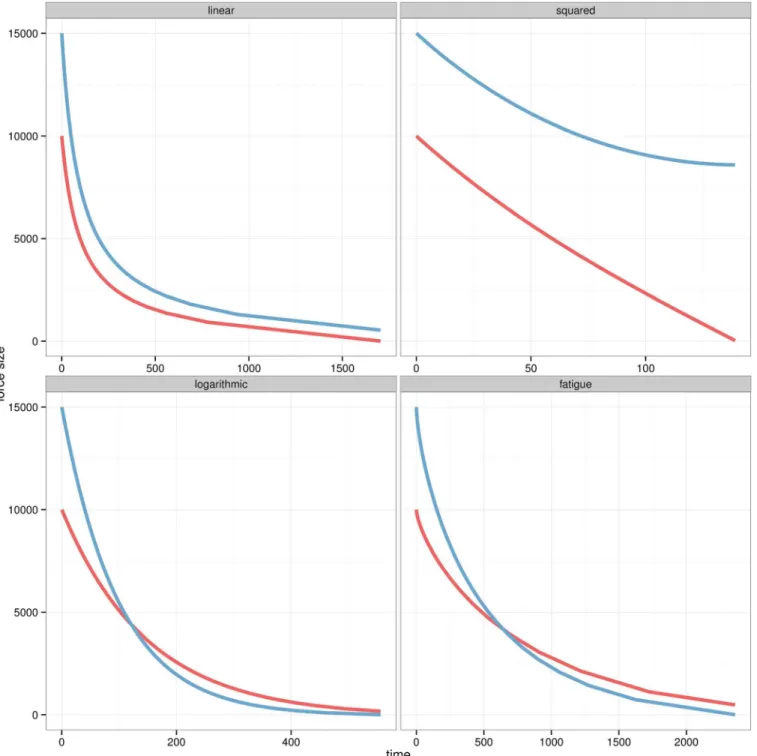
Distinctive dynamics for each model are observed inFig 3. All models are initialised as a battle where an army is being opposed by a smaller force with higher fighting value. In the lin-earmodel the forces have similar casualty rates, while size has a bigger impact in thesquared model. Thelogarithmicmodel increases the weight of fighting value over size as the smaller force finishes with more soldiers. Thefatiguemodel generates similar casualties than the loga-rithmicmodel, but they are distributed over a longer period of time.
Experiment Design
Previous authors suggested that the deterministic nature of the original laws was too rigid to perform a proper comparison with long-term observations. Using a fixedPfor a large number of battles would ignore any slight variation on the fighting value odds from one engagement to the next one. The issue has been solved introducing stochasticity inP, which is sampled every battle from a gamma distribution with shapeκand scaleθ. For convenience the input
parame-ters are expressed as meanμand standard deviationσ, which are then used to computek¼ m
s 2
andy¼s2
and initial army sizesBt= 0,Rt= 0set to historical values. The chosen Lanchester variant as
defined in Eqs4–7is then iterated until one of the forces has suffered as many casualties as recorded in the historical data. The entire workflow is depicted inFig 4.
The rejection algorithm calculates a distance between the results of a single run and observa-tions. A popular approach is the comparison of summary statistics aggregating the outcome of a run against the evidence. However, this solution has theoretical issues which are currently
Fig 4. Flowchart for the ABC framework.Example for a experiment using 1000 runs and toleranceτ= 0.01. Left side illustrates the rejection algorithm
while the green panel details the simulation of the Lanchester model.
being discussed [69]. This experiment avoids the debate by directly comparing the set of casu-alties for each battle and side. The distance between a simulation run and evidence is the abso-lute difference between simulated and historical casualties divided by historical casualties, thus normalising the weight of all battles regardless their total size. This comparison is performed identifying both in the evidence and simulation the Red armyRas the side with lower casualty ratio in each battle.
Uninformed prior beliefs were used for the two parameters (μandσ). The limits of their uniform distributions were defined asUð0
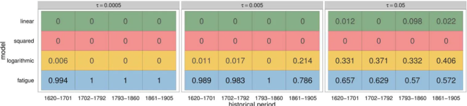
;5Þ, based on Allen’s results. Each competing model was ran 1 million times for each period. Sensitivity to tolerance levels was accounted by storing posterior distributions for different thresholds (τ= 0.05,τ= 0.005 andτ= 0.0005).
The model selection method is based on Bayes Factors. They quantify the relative likelihood of different competing models against the evidence expressed as an odds ratio [70]. This ratio was quantified with the common method of introducing a third parametermas a model index variable [59]. It was used within a hierarchical model wheremidentified which of the four vari-ants of the Lanchester’s laws was used during the run. Bayes Factors are then computed as the posterior distribution ofmwithin the tolerance levelτ.
Results
Model selection
Thefatiguemodel is decisively selected for all periods when using the lowestτ= 0.0005 (seeFig 5left). The two original models (linearandsquared) are not present in this set comprising the best 500 runs, while the logarithmic is only present for the XVIIth century. Larger tolerance levels increase the relevance of thelinearandlogarithmicmodels, while the squared model is never selected.
The estimation of distances inFig 6shows that the plausibility of the models is not constant over the different periods. The four models followed the same trend, as their ranks remain con-stant over the different phases. In addition, all of them performed much worse for the battles of the third period (i.e. Napoleonic wars).
Parameter estimation
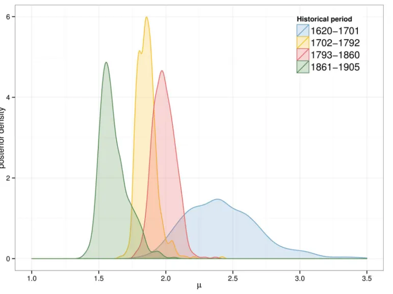
The posterior distribution for parametersμandσis now examined for thefatiguemodel at τ= 0.0005.Fig 7andFig 8show that both parameters follow unimodal distributions for all periods. The complete set of posterior distributions can be observed in SI 1, where similar pat-terns are observed for the other models (seeS1 Figfor parameterμandS2 Figfor parameterσ).
Fig 5. Model selection for different tolerance levels.Proportion of the models used in the best runs for the four historical periods and threeτvalues (corresponding to the selection of left: 500, centre: 5000 and right: 50000 best runs).
The parameterμexhibits a dynamic of gradual decrease over the three centuries. Three main blocks can be observed: the oldest period (1620–1701) has the largest mean value (2.4), while the following 150 years (second and third period) have smaller means (around 1.9) and the latest period has the lowest peak (1.6). Theσdistribution is similar for all periods except for the oldest one. The combination of the two posterior distributions as seen inFig 9illustrates the interaction betweenμandσ. The dispersion of the posterior distribution for the first period is much larger than the rest of the examined periods. In addition all results follow a distinctive pattern: the largest values ofσare only selected if theμvalue is also large.
Discussion
These results confirm that the original Lanchester’s laws (i.e.linearandsquared) are a poor match to historical evidence. The outcome is similar to other studies, which highlighted the better match of thelogarithmicmodel [51]. Beyond this replication of past results, the use of the ABC framework provides new insights to the discussion.
The decisive advantage of thefatiguemodel shows that this formulation is better supported by historical evidence than the rest of the models. The extreme psychological and physical stress conditions in the battlefield caused a gradual decrease on the efficiency of the armies. The better fit of the fourth model would suggest that this process had an impact in the final outcome. The performance of thelogarithmicmodel is similar to thefatiguemodel, even though it shows slightly lower match to evidence. The explanatory power of the two classical models is much lower, as they are consistently below the best runs for any tolerance level.
The credibility of the models is not constant over the entire time span. The best matches are the oldest and more recent periods, while the third period (1793-1860) is revealed as more unpredictable. The period was dominated by the French Revolutionary Wars and the Napole-onic Wars, where traditional European tactics were transformed at a scale not previously seen.
Fig 6. Distance from fatigue model to evidence withτ= 0.0005.Absolute distances (Y axis) of the best 500 runs ordered by rank (X axis, being 1 the best
one), model (colour) and historical period (left to right).
This outcome would suggest that the generalist approach undertaken by the Lanchester’s laws is not suited to study transition periods with higher rates of change.
Posterior distributions for parametersμandσsuggest a gradual decrease of the relevance of individual fighting value. In particular,Pvalues calculated for XVIIth century battles are larger and more diverse than the rest of the dataset. This result suggests that the non-professional armies of this era produced a much wider set of results under similar conditions, as the fighting value of the soldiers was much relevant than their numbers. The gradual standardisation of tac-tics and training would give more relevance to the size because individual fighting value was equalised between all armies. The variability of fighting valuePwithin the same period is basi-cally constant after XVIIth century. Mean values are similar for the second and third period, while showing a significant decrease after 1861. This would suggest that the evolution of war-fare, now dominated by mass-production, would give even more relevance to sheer numbers while differences between individuals would then become a minor factor.
Beyond the examined scenario, the case study illustrates howModel-Based Historycould benefit from a Bayesian-inspired framework. The use of a meta-model to compute Bayes Fac-tors allows the researcher to compare hypotheses while generating credible posterior
Fig 7. Posterior distribution ofμ.Results for thefatiguemodel andτ= 0.0005.
distributions. It also shows how the original framework can be easily extended to test new hypotheses, as seen in thefatiguemodel. It is worth mentioning that Bayes Factors already take into account parsimony because complex models with larger number of parameters will gener-ate wider posterior distributions. As a result, models with more parameters will be more times below the tolerance threshold, thus promoting simpler models.
Fig 8. Posterior distribution ofσ.Results for thefatiguemodel andτ= 0.0005.
doi:10.1371/journal.pone.0146491.g008
The study of different tolerance levels also provides a cautionary tale on the use of ABC. As its name indicates it approximates the posterior distributions, and the method needs additional parameters such as the tolerance levelτ. It means thatτalso needs to be explored, as any other parameter. Results of the case study are a good example of the need of this exploration, as Bayes Factors forτ= 0.05 are radically different than the other two values. Any study using ABC should acknowledge this issue and integrate this discussion in the experiment design.
Computational models are becoming a relevant quantitative tool for historical research. This new approach allows historians to evaluate the plausibility of competing hypotheses beyond what has been discussed in natural language. It is clear that History presents a unique set of issues and challenges to formal modelling, often related to the uncertainty of the datasets collected by the researchers. In this context, the integration of model selection methods such as ABC with new datasets and computer models can provide solutions to some of the current debates of the discipline.
Supporting Information
S1 Fig. Complete parameter estimation for parameterμ. Parameterμposterior
distribu-tion for the four models and historical periods.Results obtained from the four initial experi-ments withτ= 0.0005.
(TIFF)
S2 Fig. Complete parameter estimation for parameterσ. Parameterσposterior distribution
for the four models and historical periods.Results obtained from the four initial experiments withτ= 0.0005.
(TIFF)
S1 File. Dataset and Source code. Dataset.Dataset is distributed under the terms of a Creative Commons Attribution-ShareAlike 4.0 International License. The models and the ABC rejec-tion algorithm were implemented in Python programming language. Source code of the model is licensed under a GNU General Public License. Last versions for both data and source code can be downloaded fromhttps://github.com/xrubio/lanchester.
(ZIP)
Acknowledgments
We would like to thank Mark Madsen and two anonymous reviewers for their comments on previous versions of the manuscript. We would also like to thank Enrico R. Crema for his con-tributions in many discussions regarding the method, Victor Pascual for his suggestions on data visualization, Maria Yubero for comments on the text and Francesc Xavier Hernà ndez Cardona on the evolution of warfare.
Author Contributions
Conceived and designed the experiments: XRC. Performed the experiments: XRC. Analyzed the data: XRC. Contributed reagents/materials/analysis tools: XRC. Wrote the paper: XRC.
References
1. Epstein JM. Why model? Journal of Artificial Societies and Social Simulation. 2008; 11(4):12. Available from:http://jasss.soc.surrey.ac.uk/11/4/12.html
3. Slingerland E, Collard M. Creating consilience: integrating the sciences and the humanities. Oxford University Press; 2011.
4. Guldi J, Armitage D. The History Manifesto. Cambridge University Press; 2014.
5. Cohen D, Mandler P. The History Manifesto: A Critique. The American Historical Review. 2015; 120(2): 530–542. doi:10.1093/ahr/120.2.530
6. Armitage D, Guldi J. The History Manifesto: A Reply to Deborah Cohen and Peter Mandler. The Ameri-can Historical Review. 2015; 120(2):543–554. doi:10.1093/ahr/120.2.543
7. Currie TE, Greenhill SJ, Gray RD, Hasegawa T, Mace R. Rise and fall of political complexity in island South-East Asia and the Pacific. Nature. 2010; 467(7317):801–804. doi:10.1038/nature09461PMID: 20944739
8. Hoganson K. Computational history: applying computing, simulation, and game design to explore his-toric events. In: Proceedings of the 2014 ACM Southeast Regional Conference. ACM Press; 2014. p. 1–6.
9. Turchin P. Historical dynamics. why states rise and fall. Princeton studies in complexity. 2003;.
10. Turchin P, Whitehouse H, Francois P, Slingerland E, Collard M. A historical database of sociocultural evolution. Cliodynamics: The Journal of Theoretical and Mathematical History. 2012; 3(2).
11. Malkov AS. The Silk Roads: a Mathematical Model. Cliodynamics: The Journal of Quantitative History and Cultural Evolution. 2014; 5(1).
12. Scogings C, Hawick K. An agent-based model of the battle of Isandlwana. In: Proceedings of the Winter Simulation Conference. Winter Simulation Conference; 2012. p. 207.
13. Rubio-Campillo X, Cela JM, Cardona FXH. The development of new infantry tactics during the early eighteenth century: a computer simulation approach to modern military history. Journal of Simulation. 2013; 7(3):170–182. doi:10.1057/jos.2012.25
14. Waniek M. Petro: A Multi-agent Model of Historical Warfare. In: Web Intelligence (WI) and Intelligent Agent Technologies (IAT), 2014 IEEE/WIC/ACM International Joint Conferences on. IEEE; 2014. p. 412–419.
15. Sigrist R, Widmer ED. Training links and transmission of knowledge in 18th Century botany: a social net-work analysis. In: Redes: revista hispana para el análisis de redes sociales. vol. 21; 2011. p. 0347–387.
16. Ausloos M. On religion and language evolutions seen through mathematical and agent based models. In: Proc. First Interdisciplinary CHESS Interactions Conf; 2010. p. 157–182.
17. Bankes SC. Agent-based modeling: A revolution? Proceedings of the National Academy of Sciences. 2002; 99(suppl 3):7199–7200.
18. Schich M, Song C, Ahn YY, Mirsky A, Martino M, Barabasi AL, et al. A network framework of cultural history. Science. 2014; 345(6196):558–562. doi:10.1126/science.1240064PMID:25082701
19. Abelson RP. Statistics as principled argument. Psychology Press; 2012.
20. Gliner JA, Leech NL, Morgan GA. Problems with null hypothesis significance testing (NHST): what do the textbooks say? The Journal of Experimental Education. 2002; 71(1):83–92. doi:10.1080/ 00220970209602058
21. Nickerson RS. Null hypothesis significance testing: a review of an old and continuing controversy. Psy-chological methods. 2000; 5(2):241. doi:10.1037/1082-989X.5.2.241PMID:10937333
22. Anderson DR, Burnham KP, Thompson WL. Null hypothesis testing: problems, prevalence, and an alternative. The journal of wildlife management. 2000;p. 912–923. doi:10.2307/3803199
23. Cowgill GL. The trouble with significance tests and what we can do about it. American Antiquity. 1977; p. 350–368. doi:10.2307/279061
24. Zucchini W. An Introduction to Model Selection. Journal of Mathematical Psychology. 2000; 44(1):41–61. doi:10.1006/jmps.1999.1276PMID:10733857
25. Raftery AE. Bayesian model selection in social research. Sociological methodology. 1995; 25:111–164. doi:10.2307/271063
26. McGrayne SB. The theory that would not die: how Bayes’rule cracked the enigma code, hunted down Russian submarines, & emerged triumphant from two centuries of controversy. Yale University Press; 2011.
27. Johnson JB, Omland KS. Model selection in ecology and evolution. Trends in Ecology & Evolution. 2004; 19(2):101–108. doi:10.1016/j.tree.2003.10.013
29. Litton CD, Buck CE. The Bayesian approach to the interpretation of archaeological data. Archaeometry. 1995; 37(1):1–24. doi:10.1111/j.1475-4754.1995.tb00723.x
30. Eve SJ, Crema ER. A house with a view? Multi-model inference, visibility fields, and point process anal-ysis of a Bronze Age settlement on Leskernick Hill (Cornwall, UK). Journal of Archaeological Science. 2014; 43:267–277. doi:10.1016/j.jas.2013.12.019
31. Crema ER, Edinborough K, Kerig T, Shennan SJ. An Approximate Bayesian Computation approach for inferring patterns of cultural evolutionary change. Journal of Archaeological Science. 2014; 50:160–170. doi:10.1016/j.jas.2014.07.014
32. Buck CE, Meson B. On being a good Bayesian. World Archaeology. 2015;p. 1–18.
33. Kandler A, Powell A. Inferring Learning Strategies from Cultural Frequency Data. In: Mesoudi A, Aoki K, editors. Learning Strategies and Cultural Evolution during the Palaeolithic. Tokyo: Springer Japan; 2015. p. 85–101.
34. Will M Bertrand J, Fransoo JC. Operations management research methodologies using quantitative modeling. International Journal of Operations & Production Management. 2002; 22(2):241–264. doi: 10.1108/01443570210414338
35. Rubio-Campillo X, Hernàndez FX. An evolutionary approach to military history. Revista Universitaria de
Historia Militar. 2014; 4(2):255–277.
36. Sabin P. Simulating war: Studying conflict through simulation games. A&C Black; 2012.
37. Lanchester FW. Mathematics in warfare. The world of mathematics. 1956; 4:2138–2157.
38. Engel JH. A verification of Lanchester’s law. Journal of the Operations Research Society of America. 1954; 2(2):163–171. doi:10.1287/opre.2.2.163
39. Deitchman SJ. A Lanchester model of guerrilla warfare. Operations Research. 1962; 10(6):818–827. doi:10.1287/opre.10.6.818
40. Weiss HK. Combat Models and Historical Data: The U.S. Civil War. Operations Research. 1966; 14(5): 759–790. doi:10.1287/opre.14.5.759
41. Taylor JG. Solving Lanchester-Type Equations for“Modern Warfare”with Variable Coefficients. Opera-tions Research. 1974; 22(4):756–770. doi:10.1287/opre.22.4.756
42. Kirkpatrick DLI. Do lanchester’s equations adequately model real battles? The RUSI Journal. 1985; 130(2):25–27.
43. Lucas TW, Turkes T. Fitting Lanchester equations to the battles of Kursk and Ardennes. Naval Research Logistics. 2004; 51(1):95–116. doi:10.1002/nav.10101
44. Artelli MJ, Deckro RF. Modeling the Lanchester Laws with System Dynamics. The Journal of Defense Modeling and Simulation: Applications, Methodology, Technology. 2008; 5(1):1–20. doi:10.1177/ 154851290800500101
45. Gonzàlez E, Villena M. Spatial Lanchester models. European Journal of Operational Research. 2011; 210(3):706–715. doi:10.1016/j.ejor.2010.11.009
46. Adams ES. Lanchester’s attrition models and fights among social animals. Behavioral Ecology. 2003; 14(5):719–723. doi:10.1093/beheco/arg061
47. Shelley EL, Tanaka MYU, Ratnathicam AR, Blumstein DT. Can Lanchester’s laws help explain inter-specific dominance in birds? The Condor. 2004; 106(2):395.
48. Plowes NJR, Adams ES. An empirical test of Lanchester’s square law: mortality during battles of the fire ant Solenopsis invicta. Proceedings of the Royal Society B: Biological Sciences. 2005; 272(1574): 1809–1814. doi:10.1098/rspb.2005.3162PMID:16096093
49. Johnson DDP, MacKay NJ. Fight the power: Lanchester’s laws of combat in human evolution. Evolu-tion and Human Behavior. 2015; 36(2):152–163. doi:10.1016/j.evolhumbehav.2014.11.001
50. Jørgensen S, Sigué SP. Defensive, Offensive, and Generic Advertising in a Lanchester Model with Market Growth. Dynamic Games and Applications. 2015;.
51. Allen CD. Evolution of Modern Battle: an Analysis of Historical Data. School of Advanced Military Stud-ies; 1990.
52. Hartley DS, Helmbold RL. Validating Lanchester’s square law and other attrition models. Naval Research Logistics. 1995; 42(4):609–633. doi: 10.1002/1520-6750(199506)42:4%3C609::AID-NAV3220420408%3E3.0.CO;2-W
53. Wiper M, Pettit L, Young K. Bayesian inference for a Lanchester type combat model. Naval Research Logistics (NRL). 2000; 47(7):541–558. doi:10.1002/1520-6750(200010)47:7%3C541::AID-NAV1% 3E3.3.CO;2-S
55. Bodart G. Militär-historisches kreigs-lexikon, (1618-1905). Wien und Leipzig, C. W. Stern; 1908. Avail-able from:https://archive.org/details/bub_gb_Eo4DAAAAYAAJ
56. Weigley RF. The age of battles: The quest for decisive warfare from Breitenfeld to Waterloo. Indiana University Press; 2004.
57. Kruschke JK. Doing Bayesian Data Analysis, Second Edition: A Tutorial with R, JAGS, and Stan. Aca-demic Press; 2014.
58. Beaumont MA, Zhang W, Balding DJ. Approximate Bayesian computation in population genetics. Genetics. 2002; 162(4):2025–2035. PMID:12524368
59. Leuenberger C, Wegmann D. Bayesian Computation and Model Selection Without Likelihoods. Genet-ics. 2010; 184(1):243–252. doi:10.1534/genetics.109.109058PMID:19786619
60. Sunnåker M, Busetto AG, Numminen E, Corander J, Foll M, Dessimoz C. Approximate Bayesian Com-putation. PLoS Computational Biology. 2013; 9(1):e1002803. doi:10.1371/journal.pcbi.1002803
61. Turner BM, Van Zandt T. A tutorial on approximate Bayesian computation. Journal of Mathematical Psychology. 2012; 56(2):69–85. doi:10.1016/j.jmp.2012.02.005
62. Csilléry K, Blum MGB, Gaggiotti OE, François O. Approximate Bayesian Computation (ABC) in prac-tice. Trends in Ecology & Evolution. 2010; 25(7):410–418. doi:10.1016/j.tree.2010.04.001
63. Beaumont MA. Approximate Bayesian Computation in Evolution and Ecology. Annual Review of Ecol-ogy, Evolution, and Systematics. 2010; 41(1):379–406. doi:10.1146/annurev-ecolsys-102209-144621
64. PorčićM, NikolićM. The Approximate Bayesian Computation approach to reconstructing population dynamics and size from settlement data: demography of the Mesolithic-Neolithic transition at Lepenski Vir. Archaeological and Anthropological Sciences. 2015;p. 1–18.
65. Kovacevic M, Shennan S, Vanhaeren M, d’Errico F, Thomas MG. Simulating Geographical Variation in Material Culture: Were Early Modern Humans in Europe Ethnically Structured? In: Mesoudi A, Aoki K, editors. Learning Strategies and Cultural Evolution during the Palaeolithic. Tokyo: Springer Japan; 2015. p. 103–120.
66. Pritchard JK, Seielstad MT, Perez-Lezaun A, Feldman MW. Population growth of human Y chromo-somes: a study of Y chromosome microsatellites. Molecular Biology and Evolution. 1999; 16(12): 1791–1798. doi:10.1093/oxfordjournals.molbev.a026091PMID:10605120
67. Wegmann D, Leuenberger C, Excoffier L. Efficient Approximate Bayesian Computation Coupled With Markov Chain Monte Carlo Without Likelihood. Genetics. 2009; 182(4):1207–1218. doi:10.1534/ genetics.109.102509PMID:19506307
68. Marjoram P, Molitor J, Plagnol V, Tavare S. Markov chain Monte Carlo without likelihoods. Proceedings of the National Academy of Sciences. 2003; 100(26):15324–15328. doi:10.1073/pnas.0306899100
69. Robert CP, Cornuet JM, Marin JM, Pillai NS. Lack of confidence in approximate Bayesian computation model choice. Proceedings of the National Academy of Sciences. 2011 Sep; 108(37):15112–15117. doi:10.1073/pnas.1102900108