LARGE SCALE URBAN RECONSTRUCTION FROM REMOTE SENSING IMAGERY

LARGE SCALE URBAN RECONSTRUCTION FROM REMOTE SENSING IMAGERY

Georg Kuschk

Remote Sensing Technology Institute, German Aerospace Center (DLR), D-82234 Wessling, Germany georg.kuschk@dlr.de

KEY WORDS:Stereo, Reconstruction, Remote Sensing, Meshing, Texturing, 3D Modeling

ABSTRACT:

Automatic large-scale stereo reconstruction of urban areas is increasingly becoming a vital aspect for physical simulations as well as for rapid prototyping large scale 3D city models. In this paper we describe an easily reproducible workflow for obtaining an accurate and textured 3D model of the scene, with overlapping aerial images as input. Starting with the initial camera poses and their refinement via bundle adjustment, we create multiple heightmaps by dense stereo reconstruction and fuse them into one Digital Surface Model (DSM). This DSM is then triangulated, and to reduce the amount of data, mesh simplification methods are employed. The resulting 3D mesh is finally projected into each of the input images to obtain the best fitting texture for each triangle. As verification, we provide visual results as well as numerically evaluating the accuracy by comparing the resulting 3D model against ground truth generated by aerial laser scanning (LiDAR).

1 INTRODUCTION

Large-scale stereo reconstruction of urban areas is increasingly becoming more important in varied scientific fields as well as in common life. Applications are ranging from physical simulations like flood simulation, the propagation of radio beams or sound, to 3D change detection, flight planning for unmanned aerial ve-hicles (UAV’s), or intuitive and detailed navigation and 3D city visualization. Due to the large-scale attribute of the given prob-lem, the stereo reconstruction problem needs to be addressed with remote sensing imagery arising from satellites or aerial sensors and furthermore needs to be fully automatic, as the manual effort would render the problem intractable.

While laser scanning (LiDAR) is a very accurate method for 3D reconstruction, it does not provide any color or texture infor-mation about the scene and requires a quite expensive hardware setup. In case of satellite platforms (very large scale reconstruc-tion), laser scanning is not feasible at all. This paper is demon-strating the potential of dense stereo image matching as a cost-efficient way to create accurate and detailed textured 3D city models by the combination of current state-of-the-art computer vision methods. We further show that the accuracy of today’s optical sensors and dense stereo algorithms is indeed sufficient enough to meet the requirements of the aforementioned applica-tions - approximately 1m RMSE for aerial images (2km distance to the scene) and 3m RMSE for WorldView-2 satellite images (770km distance to the scene).

When acquiring the images, an initial pose is computed and stored along the corresponding image. In case of aerial images, data from the inertial measurement unit (IMU) and GPS information is used for estimating the initial pose. In case of satellite images, a Rational Polynomial Camera (RPC) model (see e.g. Grodecki, 2001) is initially provided for every scene. In both cases these ini-tial estimates are not very accurate, with the average re-projection error typically>1pixel. Therefore we extract and match SIFT features (Lowe, 2004) between all images and optimize the rela-tive camera poses using bundle adjustment (a survey can be found in Triggs et al., 2000) to achieve subpixel accuracy. If available, ground control point are added to the optimization process to fur-ther refine the absolute orientation of the cameras. If no initial pose is available, we compute the fundamental matrix for each image pair based on SIFT matches, and perform an image rectifi-cation on the two images.

For reconstructing the 3D scene, we use dense stereo matching to make use of all the image information and compute a depth for each single image pixel - compared to sparse multiview im-age matching methods based on SIFT- (Lowe, 2004) or SURF-like (Bay et al., 2006) features. As for each image pixel multiple depth hypotheses need to be tested, a computational efficient cost function is needed for the image matching, which additionally has to be robust to some radiometric changes between the im-ages. For this case we chose a combination of the Census trans-form (Zabih and Woodfill, 1994) and Mutual Intrans-formation (Viola and Wells III, 1997). As the pure data term of the cost function is still prone to noise and performs poorly over large disparity ranges and homogeneously textured regions, a simple pixel-wise Winner-takes-all strategy does not yield acceptable results, which is why we add additional smoothness constraints and solve the resulting optimization problem using the well established Semi Global Matching (Hirschmueller, 2005). The whole process of the 3D reconstruction is described in Section 2.1.

At this point, we have a heightmap for each input stereo image-pair, which is equivalent to a point cloud in the coordinate system of the reference image, each point also having a color assigned by it’s projection in the corresponding reference image. An interme-diate result would now be the fusion of all these point clouds into an even denser point cloud. However, for our purpose, we trans-form the different heightmaps (respectively their point clouds) into a common orthographic coordinate system (UTM coordinate system) and due to a large image overlap and therefore redun-dant height information, fuse the projected Digital Surface Mod-els (DSMs) into one single DSM, yielding a higher accuracy be-cause of reduced noise. Since all of our applications need a closed surface, we afterwards transform this DSM (or point cloud) into a meshed 3D model by Delaunay triangulation (Guibas and Stolfi, 1985).

match-ing of sparse image features, whereas in our approach the reduc-tion takes place at a later step and uses all the dense depth infor-mation to detect and simplify local planar surfaces. And to finally get a visually appealing and realistically textured 3D model, we use images of the scene taken from different viewpoints to assign best fitting textures for all triangles of the 3D model. The process of the automatic 3D modeling is described in Section 2.3. For evaluation of the algorithm’s accuracy, we provide both vi-sual and numerical results for two test scenes of urban areas as described in Section 3. Test scene A consists of an aerial im-age set of the city of Munich, while Test scene B consists of WorldView-2 satellite images of London. The results of both data sets are numerically evaluated against reference data obtained by airborne laser scanning (LiDAR) - see Section 4.

2 METHOD

In Figure 1, an overview of the complete workflow of the pro-posed method is shown - starting with a number of input images Iktogether with their initial camera posesCk.

Bundle adjustment

Pairwise dense stereo matching

Fuse to single DSM

Meshing + Mesh simplification

Multiview texturing

3D point cloud

Textured 3D mesh

Figure 1: Workflow of the 3D reconstruction process withninput imagesIkand camera posesCk, refined camera posesCk∗and

n−1pairwise heightmapsHMk.

As already mentioned in the introduction, we first refine the initial poses to achieve subpixel accuracy for the dense stereo match-ing. To this end we extract and match SIFT features between all images and optimize the relative camera poses using bundle adjustment. If available, ground control point are added to the optimization process to further refine the absolute orientation of the cameras.

2.1 Dense Stereo Reconstruction

In classical dense stereo reconstruction, for every image pixel of the reference image(x, y)∈I1and a number of height/depth hy-pothesesγ∈Γ, a matching cost is computed by back-projecting the pixel into 3D space, projecting the resulting 3D point into the second image→(x′

, y′

) ∈ I2and comparing the image infor-mation of the two images at their corresponding positions. The result is the so calleddisparity space image(Bobick and Intille, 1999), containing therawmatching costs.

If no information about the camera model would be available, the search space for matching one pixel in imageI1would be the the whole imageI2. To reduce the search space from 2D to 1D, we

need to establish an epipolar geometry between image pairs. If the cameras can be approximated by the pinhole camera model, the resulting epipolar geometry is mapping one image coordinate in the first image to a corresponding line in the second image. However, satellite images are obtained using a push-broom cam-era (the CCDs are arranged one-dimensional instead of a two-dimensional array) and the resulting epipolar lines of an image pair using the corresponding Rational Polynomial Camera (RPC) model are not straight, but curved (Oh, 2011).

We therefore pursue a different strategy and establish the epipo-lar geometry between two imagesI1andI2directly by evaluating the functionF(1,2)(x, γ), which projects a pixelxfromI1toI2

using the disparityγ, for every single pixel ofI1∈Ωand every possible disparityγ∈Γindividually. As the camera model may be very complex and computationally expensive andΩ×Γquite large, we computeF(1,2)(x, γ)only for a sparse (and uniformly

distributed) set of grid points inΩ×Γspace and store the results in a lookup-table. For all other points we compute the projected pixel by trilinear interpolation of the nearest grid points. By embedding this procedure in a plane-sweep approach (Collins, 1996), we furthermore get a rotational invariant cost function without introducing additional efforts. Given a disparityγ, we sweep over the reference imageI1, sample imageI2at the cor-responding image position(x′

, y′

)and copy the obtained color / intensity to an imageI2˜ at the same position(x, y)as in the reference image. When computing the matching costs of a dis-parity hypothesesγand the whole imageI1, we simply evaluate the cost function at the same position(x, y), using the same local support window in bothI1andI2(see Figure 2).

Note that by using this approach we have no need for an image rectification and avoid the errors induced by projective distortions and the involved sampling and interpolation.

Figure 2: Computation of the disparity space image using a plane-sweep approach: For a coordinate(x, y)in imageI1 and disparityγ, obtain the corresponding coordinate(x′

, y′

)in image I2using the camera modelF1,2, sample the pixel color/intensity and copy it to thewarpedimageI2˜ at position(x, y). The match-ing cost can then be computed by comparmatch-ing the pixel intensities in both images at position(x, y).

2.1.1 Cost Function As cost function for the image matching we chose the Census transform (Zabih and Woodfill, 1994) and afterwards perform a (very small) local aggregation of it using Adaptive support-weights (Yoon and Kweon, 2006).

inten-sity order:

ξ(I(x), I(x′)) = 

1 if I(x′)< I(x)

0 otherwise (1)

CT(I,x) = O

[i,j]∈D

ξ(I(x), I(x+ [i, j])) , (2)

with the concatenation operator N

and an ordered set of dis-placementsD ⊂ R2, which is normally chosen to be a7×9 window. Because due to implementation issues, the resulting bi-nary vector of length 63 fits into a 64 Bit variable. The matching cost of different Census vectorss1, s2is then computed as their Hamming distancedH(s1, s2)– number of differing bits – where

highest matching quality is achieved for minimal Hamming dis-tance, and the costs are normed to the real-valued interval[0,1]

cost(x, γ) =

dH`CT(I1,x), CT(I2, F(1,2)(x, γ))´

maxi,j{dH(si, sj)}

(3)

Using such a7×9support window for the Census transform increases the robustness of the matching function against mis-matches, especially when searching through a large disparity range as is very common in remote sensing data.

On the other hand, this window-based matching suffers from the ”foreground fattening” phenomenon when support windows are located on depth discontinuities, such as partially covering a roof top and the adjacent street. To limit this effect, we locally ag-gregate the cost function of Equation (3) using adaptive support-weights (Yoon and Kweon, 2006) for corresponding pixelspin I1andqinI2:

C(p, q) =

P

˜

p∈Np,q˜∈Nq[w(p,p)˜ ·w(q,q)˜ ·cost(˜p,q)]˜

P

˜

p∈Np,q˜∈Nq[w(p,p)˜ ·w(q,q)]˜

(4)

The weightsw(p, q)are based on color differences∆c(p, q)and

spatial distances∆d(p, q)

w(p, q) = exp

„

−∆c(p, q)

γc

−∆d(p, q)

γd «

(5)

withγd = 5(= radius of the support window) andγc = 5.0

for 8-bit images (respectivelyγc = 20.0for 11-bit images). As

this local aggregation favors fronto-parallel surfaces, we keep this radius relatively small (4 pixel), to keep a balance between in-creased accuracy along discontinuities and not ”over-favoring” fronto-parallel surfaces.

(a) (b)

Figure 3: a) The7×9windowDof the Census transform, b) The basic scheme for the adaptive support-weights.

2.1.2 Optimization In the resulting disparity space image (DSI) we now search for a functionalu(x)(the disparity map), which

minimizes the energy function arising from the matching costs (called data termEdata), plus additional regularization terms. As

the data term is prone to errors due to some incorrect and noisy measurements, one often needs some smoothness constraintsEsmooth,

forcing the surface of the disparity map to be locally smooth.

u(x) = argmin u

Z

Ω

Edata+Esmoothdx ff (6) = argmin u Z Ω

C(x, u(x)) +∇u(x)dx ff

This energy is non-trivial to solve, since the smoothness con-straints are based on gradients of the disparity map and therefore cannot be optimized pixelwise anymore. Various approximations for this NP-hard problem are existing, e.g. Semi-global Match-ing (Hirschmueller, 2005), energy minimization via graph cuts (Boykov et al., 2001) or minimization of Total Variation (Pock et al., 2008) - just to name three examples. Because of its simple implementation, low computational complexity and good regu-larization quality, we use semi-global matching for optimization, minimizing the following discrete energy term

E(u) =X

x

C(x, u(x)) +

X

p∈Nx

P1·T[|u(x)−u(p)|= 1] +

X

p∈Nx

P2·T[|u(x)−u(p)|>1] (7)

The first term is the matching cost, the second and third term penalties for small and large disparity discontinuities between neighboring pixelsp∈Nx. The key idea is now not to solve the

intractable global 2D problem, but to approximate it by combin-ing 1D solutions from different directionsr, solved via dynamic

programming

u(x) = argmin u

( X

r

Lr(x, u(x) )

(8)

The aggregated costLr(x, u(x))in Equation (8) represents the

cost of pixelxwith disparityd=u(x)along the directionrand

is being computed as

Lr(x, d) =C(x, d) + min(Lr(x−r, d),

Lr(x−r, d−1) +P1, Lr(x−r, d+ 1) +P1,

min

k Lr(x−r, k) +P2) − mink Lr(x−r, k)

(9)

The penalties are set to default valuesP1 = 0.4andP2 = 0.8 (with the raw costs normed to[0,1]). For deeper insights the reader is referred to the paper of Hirschmueller, 2005.

2.2 DSM Post-Processing

After obtaining the disparity map for each image pair, there are most certainly some errors / outliers left due to mismatches or occlusions. To further reduce the number of outliers and increase the accuracy of the disparity map, we apply the following post-processing steps:

• Consistency check

dispar-ity at this position is considered to be invalid

D1(x) =

 D₁(x)+D2(x)

2 if |D1(x)−D2(x)|< θLR invalid otherwise

(10)

Note that this requires twice the time of the overall algo-rithm, since two disparity maps have to be computed.

• Median filtering

Removing additional noise / small area outliers by filtering the disparity map with a3×3median filter

• Interpolation

The invalidated disparities, resulting from occlusions and mismatches, need to be interpolated, which is mostly done based on the disparities in the local neighborhood. To this end, we implemented and use the multilevel interpolation based on B-splines from (Lee et al., 1997).

• Subdisparity accuracy

By fitting a quadratic curve through the cost of the obtained disparityC(x, d)and the costs of the adjacent disparities

(±1) and computing the minimum of this curve, we refine the disparity map to subdisparity accuracy. Note that this is theoretically only valid for SSD-based cost functions, but nevertheless works fine for most cost functions.

• Multiview DSM fusion

In the case of two input images, we just project the single disparity map into UTM coordinate system, discretize the result and again interpolate the hereby invalidated areas in the DSM (areas of the DSM which are occluded in the dis-parity map).

For more than two input images, we compute a disparity map for each image pair and project all of them into a reg-ular spaced and discretized grid given in UTM coordinate system. By collecting all the height values per DSM-pixel, we afterwards choose the median of these to be our final height value of the DSM at this position.

2.3 3D Modeling

2.3.1 Meshing We create a triangulated mesh of the DSM by simply connecting four incident pixels(x, y),(x+ 1, y),(x+ 1, y+ 1),(x, y+ 1)into two triangles. Of the two possible tri-angulations we choose the one which better matches the height information by using an adaptive triangulation method minimiz-ing the second derivative of the surface in the neighborhood of the square, as proposed in Grabner, 2002.

2.3.2 Simplification Using the naive meshing from above, the triangulated mesh roughly contains2ntriangles, ifnis the num-ber of pixels in the DSM. As our aerial image data for example has a resolution of0.2m, our 3D model would have about 25 tri-angles per m2 or25·106 triangles per km2 - which is simply too much for our purposes. Therefore, we further employ a two step mesh simplification to reduce the amount of triangles needed to represent the 3D model, while at the same time preserving its dominant features and surface properties.

The first step aims at simplifying planar structures. To this end, we iterate over all vertices and fit a 3D plane through its adjacent neighbors using the least squares method. Using a quad-edge data structure as in Guibas and Stolfi, 1985 allows an efficient search for the neighboring vertices.

If the minimum distance of the currently visited vertex to the fit-ted plane is<∆plan, the vertex is deemed to be redundant and

marked for removal (see Figure 4). As this would sometimes

remove the corners of steep building walls, we add a further con-straint that the vertex gets only removed, if the height difference to all of its adjacent vertices is<∆disc. These two parameters

depend on the grid resolutionδof the initial DSM and were cho-sen to be∆plan = δand∆disc = 10δ. An evaluation of the

influence of this parameterδis conducted in Section (4), Figure (10).

The second step of our mesh simplification is removing nearly collinear triangles. If for any triangle(A, B, C),AB+AC < BC·∆coll(with∆coll>1) the vertexAwill be removed. We

chose to remove only very collinear triangles (∆coll= 1.01).

(a) (b)

Figure 4: a) Planar mesh simplification, b) Collinear mesh sim-plification

2.3.3 Multi-view texturing Using a single image for textur-ing is done straightforward: We project each triangle of our 3D model into the image plane, check whether the 2D projection faces towards the given camera and store the projected 2D im-age coordinates as normalized texture coordinates.

However, images of the scene taken from different viewpoints al-low us to extract the texture of parts of the scene hidden from a single view, like for example the facades of buildings (see Figure 5). In that case we have to devise a quality measureQfor the projectionπ(ti, Ik)of a triangletiinto each imageIkavailable

for texturing. Of all theseKprojections, we then choose the one with the best quality measure for texturing the triangleti

k= argmax

k

{Q(π(ti, Ik) )} (11)

Figure 5: Multi-view texturing

the camera.

We therefore extract a texture for a triangletifrom the imageIk,

where its projection on the image plane is maximal and simul-taneously least occluded by other projected triangles. To solve these requirements efficiently, we compute the texture quality of each triangle for an imageIkusing the following z-buffering

ap-proach:

• Sort all 3D triangles of the model according to the distance to the camera center

• Beginning with the furthest triangle, compute the projection of all triangles onto the image plane and render them using a unique identifier / unique color each

• Sweep over the rendered image and compute the visibility of each triangle in term of its remaining visible pixels:

Q(π(ti, Ik)) = X

(x,y)∈π 

1 (x, y) visible 0 otherwise

ff

(12)

Using equation 11, we obtain the view where the best texture quality is to be expected and store the corners of the triangle’s 2D projection as its texture coordinates.

3 DATA

For evaluation, two test sites of complex urban areas were cho-sen (see Figure 6 and 7), both covering an area of2000×2000 pixel. The two test sites were captured with different remote sens-ing sensors and ground truth data was obtained by airborne laser scanning (LiDAR) in both cases.

3.1 Aerial image data - Munich

The aerial image data was taken of the inner city of Munich, using the 3K+ camera system (Kurz et al., 2007). The flight altitude (or distance of the camera to the scene) is≈2km above ground with a ground sampling distance (GSD) of≈ 0.2m per pixel. 17 partially overlapping images (converted to gray scale, 8 Bit per pixel) were used for the 3D reconstruction, and for texturing, the RGB images themselves were used. The resulting DSM is resampled to0.2m and, having a size of2000×2000pixel, covers an area of400m×400m.

3.2 Satellite image data - London

The satellite image data was taken of the inner city of London, us-ing the WorldView-2 satellite. The flight altitude (or distance of the camera to the scene) is≈770km above ground with a ground sampling distance (GSD) of0.5m per pixel. 8 overlapping im-ages (obtained during one pass) of the panchromatic sensor (11 Bit per pixel) were used for the 3D reconstruction. For texturing, RGB images were computed by pansharpening the 0.5m GSD panchromatic images with the 2.5m GSD multispectral channels. The resulting DSM is resampled to0.5m and, having a size of 2000×2000pixel, covers an area of1km×1km.

4 RESULTS

For both test areas, reference data was obtained by airborne laser scanning (LiDAR), having a positional resolution of about1m, a positional accuracy of0.5m RMSE and a vertical accuracy of 0.25m RMSE according to the provider of the data. Due to the different resolution of the DSMs and the LiDAR point cloud, we

Figure 6: Aerial image data - inner city of Munich (Marienplatz)

Figure 7: Satellite image data - inner city of London (Canary Wharf)

compute the error metrics as Euclidean distance between the Li-DAR points and the triangulated surface of the DSMs and 3D models.

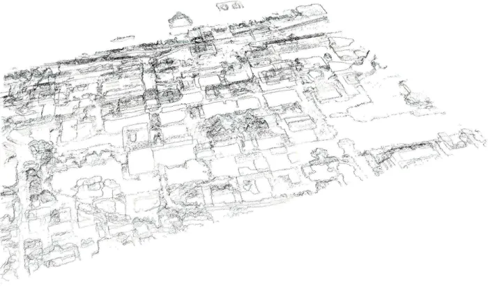
(a) Aerial image data - Thinned point cloud

(b) Aerial image data - Textured mesh

(a) Satellite image data - Thinned point cloud

(b) Satellite image data - Textured mesh

Table 1: Properties of the two data sets and accuracy of the result-ing DSMs and 3D models - Mean Absolute Error (MAE), Root Mean Square Error (RMSE), Normalized Median Absolute De-viation (NMAD)

Munich 3K+ London WV2

Area [pixel] 2000×2000 2000×2000

GSD [m] 0.2 0.5

Area [m] 400×400 1000×1000

Vertices in 3D model 221,000 103,000

Vertices / m2 1.38 0.10

Vertices / pixel 0.06 0.03

DSM - MAE [m] 0.71 1.17

DSM - RMSE [m] 1.44 2.07

DSM - NMAD [m] 0.52 0.78

3D Model - MAE [m] 0.86 1.69

3D Model - RMSE [m] 1.51 2.44

3D Model - NMAD [m] 0.77 1.62

0 0.2 0.4 0.6 0.8 1

0.5 1 1.5 2 2.5 3 3.5 4 4.5x 10

5

#vertices

δ

0 0.2 0.4 0.6 0.8 11.2

1.3 1.4 1.5 1.6 1.7 1.8 1.9 2 MAE [m]

Figure 10: Influence of the mesh simplification parameterδon the accuracy of the resulting 3D model (London data set). The correlation between the reduced number of vertices and increas-ing mean absolute error is clearly visible.

5 CONCLUSION

In this paper we presented a complete, fully automatic and model-free workflow for the 3D reconstruction of large scale (urban) ar-eas. As our focus is on fully automatic processing chains, we can process the input image data very fast, around the clock and without the need for additional user-guided input. Of course, with manual interaction the accuracy normally is better than a fully au-tomatic approach, so if there is need for higher accuracy, the re-sulting 3D models can be refined later on by further (semi-) man-ual processing. We additionally point out that, except from the input images themselves, no additional data like building foot-prints, special building models / primitives, road maps, etc. is required.

The accuracy was shown to be in the range of about 1m mean absolute error and about 2m root mean square error (mainly in height) for images with a GSD (or pixel size) of0.2-0.5m, taken from 2km and 770km distance to the scene. Compared to our LiDAR ground truth’s horizontal accuracy of0.5m RMSE and vertical accuracy of0.25m RMSE, the results of our image-only reconstruction is not that far off.

ACKNOWLEDGMENTS

The author would like to thank European Space Imaging (EUSI) for providing the WorldView-2 data of London.

REFERENCES

Bay, H., Tuytelaars, T. and Van Gool, L., 2006. Surf: Speeded up robust features. ECCV pp. 404–417.

Bobick, A. and Intille, S., 1999. Large occlusion stereo. Interna-tional Journal of Computer Vision 33(3), pp. 181–200. occlusion detection.

Boykov, Y., Veksler, O. and Zabih, R., 2001. Fast approximate energy minimization via graph cuts. IEEE Transactions on pat-tern analysis and machine intelligence pp. 1222–1239. Graph Cuts.

Collins, R., 1996. A space-sweep approach to true multi-image matching. In: cvpr, Published by the IEEE Computer Society, p. 358.

Grabner, M., 2002. Compressed adaptive multiresolution encod-ing. Journal of WSCG 10(1), pp. 195–202.

Grodecki, J., 2001. Ikonos stereo feature extraction - rpc ap-proach. In: Proc. ASPRS Annual Conference, St. Louis, pp. 23– 27.

Guibas, L. and Stolfi, J., 1985. Primitives for the manipulation of general subdivisions and the computation of voronoi diagrams. ACM Transactions on Graphics 4(2), pp. 74–123.

Hirschmueller, H., 2005. Accurate and efficient stereo processing by semi-global matching and mutual information. In: Computer Vision and Pattern Recognition, 2005. CVPR 2005. IEEE Com-puter Society Conference on, Vol. 2, IEEE, pp. 807–814.

Kurz, F., Mueller, R., Stephani, M., Reinartz, P. and Schroeder, M., 2007. Calibration of a wide-angle digital camera system for near real time scenarios. In: Proc. ISPRS Hannover Workshop 2007-High Resolution Earth Imaging for Geospatial Information, pp. 1682–1777.

Lee, S., Wolberg, G. and Shin, S., 1997. Scattered data inter-polation with multilevel b-splines. Visualization and Computer Graphics, IEEE Transactions on 3(3), pp. 228–244.

Lowe, D., 2004. Distinctive image features from scale-invariant keypoints. International Journal of Computer Vision 60(2), pp. 91–110.

Oh, J., 2011. Novel Approach to Epipolar Resampling of HRSI and Satellite Stereo Imagery-based Georeferencing of Aerial Im-ages. PhD thesis, The Ohio State University.

Pock, T., Schoenemann, T., Graber, G., Bischof, H. and Cremers, D., 2008. A convex formulation of continuous multi-label prob-lems. Computer Vision - ECCV 2008 pp. 792–805.

Triggs, B., McLauchlan, P., Hartley, R. and Fitzgibbon, A., 2000. Bundle adjustment - a modern synthesis. Vision algorithms: the-ory and practice pp. 153–177.

Viola, P. and Wells III, W., 1997. Alignment by maximization of mutual information. International journal of computer vision 24(2), pp. 137–154.

Yoon, K. and Kweon, I., 2006. Adaptive support-weight ap-proach for correspondence search. Pattern Analysis and Machine Intelligence, IEEE Transactions on 28(4), pp. 650–656.