On microphysical processes of noctilucent clouds (NLC): observations and modeling of mean and width of the particle size-distribution

(1)

ACPD

10, 3605–3625, 2010

Size and distribution width of NLC

G. Baumgarten et al.

Title Page

Abstract Introduction

Conclusions References

Tables Figures

◭ ◮

Back Close

Full Screen / Esc

Printer-friendly Version

Interactive Discussion Atmos. Chem. Phys. Discuss., 10, 3605–3625, 2010

www.atmos-chem-phys-discuss.net/10/3605/2010/ © Author(s) 2010. This work is distributed under the Creative Commons Attribution 3.0 License.

Atmospheric Chemistry and Physics Discussions

This discussion paper is/has been under review for the journal Atmospheric Chemistry and Physics (ACP). Please refer to the corresponding final paper in ACP if available.

On microphysical processes of

noctilucent clouds (NLC): observations

and modeling of mean and width of the

particle size-distribution

G. Baumgarten, J. Fiedler, and M. Rapp

Leibniz-Institut f ür Atmosph ärenphysik e.V., 18225 K ühlungsborn, Germany

Received: 11 December 2009 – Accepted: 25 January 2010 – Published: 9 February 2010

Correspondence to: G. Baumgarten ([email protected])

(2)

ACPD

10, 3605–3625, 2010

Title Page

Tables Figures

◭ ◮

Back Close

Full Screen / Esc

Interactive Discussion

Abstract

Noctilucent clouds (NLC) in the polar summer mesopause region have been observed in Norway (69◦N, 16◦E) between 1998 and 2009 by 3-color lidar technique. Assuming a mono-modal Gaussian size distribution we deduce mean and width of the particle sizes throughout the clouds. We observe a quasi linear relationship between

distribu-5

tion width and mean of the particle size at the top of the clouds and a deviation from this behavior for particle sizes larger than 40 nm, most often in the lower part of the layer. The vertically integrated particle properties show that 65% of the data follows the linear relationship with a slope of 0.42±0.02. For the vertically resolved particle properties (∆z=0.15 km) the slope is smaller and only 0.39±0.03. We compare our

10

observations to microphysical modeling of noctilucent clouds and find that the distribu-tion width depends on turbulence, the time that turbulence can act (cloud age), and the sampling volume/time (atmospheric variability). The model results nicely reproduce the measurements and show that the observed slope can be explained by eddy di_ffusion profiles as observed from rocket measurements.

15

1 Introduction

Noctilucent clouds (NLC; also called polar mesospheric clouds, or PMC, when seen from space) are an intriguing optical twilight phenomenon which can be observed throughout the summer months, most often at latitudes poleward of 50◦(e.g., Thomas, 1984; Gadsden and Schr ¨oder, 1989). NLC consist of water ice particles which form

20

in the extremely cold and dry environment of the polar summer mesopause region (Hervig et al., 2001). This region is characterized by mean temperatures being as low as∼130 K and by water vapor mixing ratios of just a few parts per million by volume (ppmv) (e.g., L ¨ubken, 1999; Seele and Hartogh, 1999). Temperature and water vapor in the polar summer mesopause region are driven by dynamical processes from global

25

(3)

ACPD

10, 3605–3625, 2010

Title Page

Tables Figures

◭ ◮

Back Close

Full Screen / Esc

Interactive Discussion which can be seen directly in NLC displays (Witt, 1962; Fritts et al., 1993). Existing just

at the edge of feasibility, NLC properties are extremely sensitive toward changes of their environment (e.g., temperature, water vapor, or dynamical parameters like wave activity). We report on observations of particle properties by multi-color lidar performed in Northern Norway (Baumgarten et al., 2008). We investigate in detail the mean and

5

the width of the size distribution and compare the results to microphysical modeling of NLC to identify the processes affecting especially the distribution width. Besides the microphysical aspects these observations are important for the interpretation of other instruments sounding the particle size of NLC. For most instruments the particle size is retrieved under the assumption of a predefined and constant distribution width (e.g.,

10

Bailey et al., 2009; Robert et al., 2009). From our measurements we show that this assumption needs to be revisited.

In the following section we will briefly describe the observation method, including the data analysis procedure, and the microphysical model focused on the sensitivity study used for interpretation of the observations. In Sect. 3 we will present the observations

15

and in Sect. 4 we will discuss the observations as well as the underlying microphysical processes.

2 Instrument, method and model 2.1 Lidar

Lidar measurements of NLC particle properties were performed with the ALOMAR

20

RMR-lidar in Northern Norway (69◦N, 16◦E). Throughout the NLC season (1 June– 15 August) from 1998 to 2009 the lidar was operated whenever permitted by the weather. Laser pulses at three widely separated wavelengths (355 nm, 532 nm, 1064 nm) are emitted, scattered back by air molecules and particles in the atmo-sphere and collected by telescopes with a diameter of 1.8 m. The received light

25

(4)

ACPD

10, 3605–3625, 2010

Title Page

Tables Figures

◭ ◮

Back Close

Full Screen / Esc

Interactive Discussion molecular signal, the particle properties are calculated by comparison to modeled

optical particle signals (Baumgarten et al., 2007). The method is appropriate for the analysis of a mono-modal size distribution consisting of non-spherical particles, where the radius is that of a volume-equivalent sphere. Throughout this manuscript we use results for an assumed Gaussian-shaped size distribution (Berger and von

5

Zahn, 2002; Rapp and Thomas, 2006). We analyze the particle properties through-out the NLC layer where the NLC signal is larger than twice the measurement uncer-tainty: β532nm,NLC(z)>2·∆β532nm,NLC(z), with β being the backscatter coefficient and

∆βthe corresponding measurement uncertainty. The measurements of NLC are an-alyzed for particle sizes only when in addition the measurement errors of the color

10

ratios CR_λ,_NLC=βλ,NLC/β532nm,NLC are small. In detail: ∆CR1064nm,NLC(z)<0.08 and

∆CR355nm,NLC(z)<1.0.

To enhance the signal to noise ratio, the data throughout the layer are processed in different ways: Minimal averaging using a sliding binomial filter with FWHM=475 m and 150 m sampling (method 1). Segmentation of the layer into upper, peak and lower part

15

(method 2). Usage of the vertically integrated signal (method 3). Further details on the analysis of the vertical structure throughout the NLC layer can be found in Baumgarten and Fiedler (2008). While method 1 shows the particle properties at the highest possi-ble resolution, method 3 should be more comparapossi-ble to other sounding methods (e.g. nadir viewing satellite instruments). Method 2 allows to study different aspects of the

20

cloud microphysics. As the cloud particles fall through the atmosphere while they grow, younger particles should be found above the peak of the layer, while mature particles are expected at the layer bottom.

2.2 CARMA

The community aerosol and radiation model for atmospheres (CARMA) is a

micro-25

(5)

ACPD

10, 3605–3625, 2010

Title Page

Tables Figures

◭ ◮

Back Close

Full Screen / Esc

Interactive Discussion was first applied to the physics of mesospheric ice particles by Turco et al. (1982), and

then further developed by several authors (e.g., Jensen and Thomas, 1994; Rapp et al., 2002). For the current study, we use results from a large number of simulations using a 1-D version of CARMA which have been described in detail in Rapp and Thomas (2006); Rapp et al. (2007).

5

3 Observations

The ALOMAR RMR-lidar has been operated for 3972 h during the NLC seasons from 1998 to 2009 whereof about 1680 h contain signatures of NLC. A detailed description of the NLC dataset and the mean particle properties can be found in Fiedler et al. (2009) and Baumgarten et al. (2008), respectively. The lidar is designed as a twin system and

10

measurements can be performed at two different locations separated by about 40 km at NLC altitude (Baumgarten et al., 2002). For the particles soundings we treat these as independent observations. This data set was analyzed with a temporal resolution of 14 min. In total this results in 22 820 soundings that could be analyzed for particle properties. Due to instrument developments the number of particle size soundings has

15

increased since 2005. About 92% of the size measurements were performed in the years 2006–2009.

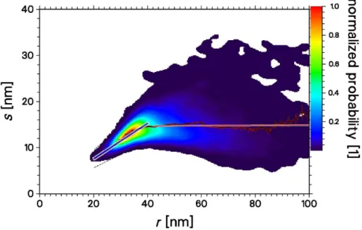
In Fig. 1 we show the retrieved width (s) and the mean (r) of the particle size dis-tribution, color-coded as 2-D probability distribution relative to the maximum. The fig-ure shows results for the total dataset sampled with the highest possible resolution

20

(method 1). The ensemble of particles with r=31 nm ands=13 nm occur most often and hence show the highest probability density. The mean distribution width for diff er-ent particle sizes, calculated by binning the sizes in 2.5 nm steps, is also shown in the figure. We find two different relationships between distribution width and mean radius: for particle sizes below 40 nm width and radius are strongly correlated, while for larger

25

(6)

ACPD

10, 3605–3625, 2010

Title Page

Tables Figures

◭ ◮

Back Close

Full Screen / Esc

Interactive Discussion The weight of the regression is defined by the measurement uncertainty, in case of

the size-binned mean (black-red curve in Fig. 1) we use the statistical error of the mean. The resulting slopes areS_<40nm=0.39±0.03 forr<40 nm andS≥40nm=0.003±0.008 for r≥40 nm. We observe a strong dependence of s and r for mean sizes below about 40 nm, while the mean distribution width is constant at abouts=(14.7±1.5) nm for

par-5

ticles from 40 to 100 nm.

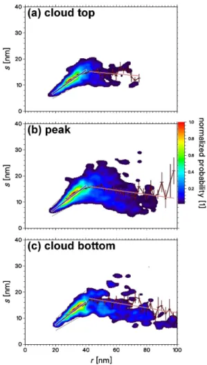
We have investigated the s/r behavior for different parts of the layer (method 2), as it is shown by observations and model simulations that there is a strong vertical dependence of the particle properties (e.g., von Savigny et al., 2005; Hervig et al., 2009; Baumgarten and Fiedler, 2008). The results are shown in Fig. 2. The mean

10

vertical extent of the NLC top, peak and bottom parts are 0.92 km, 0.76 km and 0.65 km, respectively. For all layer parts we find a strong correlation ofsandr for mean sizes up to 40 nm. The slope varies only slightly throughout the layer from 0.41 to 0.44 for the cloud top and bottom, respectively. At the mean size of aboutr=40 nm the relationship betweens and r changes and we find a decrease of the mean distribution width with

15

increasingr. To estimate how well the mean slope describes the whole dataset we have calculated the fraction of particle soundings that deviate by more than 25% from

s/r=S<40nm. We find that 79% (top), 63% (peak) and 51% (bottom) of all particle

soundings are compatible with the mean slope (S_<40nm). Deviations from the mean

slope are mostly caused by larger particles located below the mean slope.

20

We have investigated the vertical mean particle properties by averaging the signal over the full altitude range (method 3). In Fig. 3 the vertical extent of the sounding volume is about 3...10 times larger than in Fig. 1 and includes the vertical gradient of the mean particle sizes (c.f. Fig. 6). Nevertheless we also find for the vertically inte-grated signal that about 65% of the observations are compatible with the mean slope

25

of S<40nm=0.42±0.02. The results for the different analysis methods applied to the

(7)

ACPD

10, 3605–3625, 2010

Title Page

Tables Figures

◭ ◮

Back Close

Full Screen / Esc

Interactive Discussion Fig. 1 to Fig. 3 shows that the methods 1 and 3 – both calculating the average relation

betweensandr for the whole NLC observations – produce different results. For exam-ple the slopeS_≥40nmis zero for method 1 butS≥40nm=−0.08±0.02 for method 3. The

underlying reason is that for method 3 particle properties at the bottom of the cloud have a higher weight as for method 1. For method 1 all particle properties throughout

5

the layer have the same weight, independent of the particle size. It should be noted that the vertical weighting function depends on the instrument (wavelength) used to derive particle properties (e.g., Hervig et al., 2009).

Additionally we have performed the analysis separately for different NLC brightness classes (e.g., Fiedler et al., 2003). We observe a similar slope for all cloud classes

10

and do not find a significant difference for weak to strong clouds. The slope depends slightly on the analysis method where the smallest sounding volume (method 1: 475 m FWHM smoothing length) shows the lowest slope, about 10% smaller than the slope of the vertically integrated layer. From weak to strong clouds the number of particle soundings that follow the mean slope varies from 89% for weak clouds to only 33%

15

for strong clouds at the NLC bottom. The results for the different analysis methods and cloud classes are compiled in Table 2. The distribution widths for two fixed mean particle sizes (35 nm and 50 nm) are explicitly listed in the table. The widths for 35 nm mean sizes for analysis methods 2 and 3 are usually larger than that of method 1, which uses the highest vertical resolution and hence the smallest sounding volume.

20

4 Model results and discussion

We have analyzed CARMA simulations for 792 different combinations of temperature, H2O and eddy diffusion (turbulence) to study the effect of background variability on the

NLC particle properties. These are the same model runs as previously described and discussed by Rapp et al. (2007) in the context of modeling color ratios observed by

25

lidar. The key questions to be addressed with the help of these model runs were: (1) What is the cause for the increase of distribution width with increasing particle

(8)

ACPD

10, 3605–3625, 2010

Title Page

Tables Figures

◭ ◮

Back Close

Full Screen / Esc

Interactive Discussion (2) What parameters do determine the slope of this increase?

(3) Why does the distribution width stop growing at about 40 nm?

(4) What process does cause a decrease of distribution width for large particles?

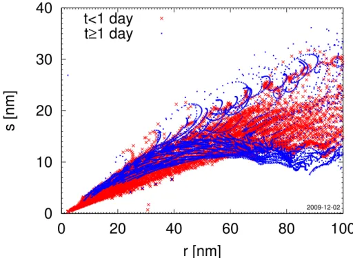
In Fig. 4 we show the model results for varying temperature and H2O but the turbulent

eddy diffusion profile of the reference case, discussed in detail in Rapp and Thomas

5

(2006). We observe that the model shows a correlation of mean and width, similar to the lidar observations. In the model the distribution width increases until the mean particle size has reached about 60 nm. Furthermore we observe that the distribution width decreases for larger particles for “mature” clouds i.e., after more than one day of model simulation. This result is compatible to the lidar observations where we find the

10

deviations from the correlation of width and mean size in the lower part of the layer. Here we expect to find the oldest (“mature”) particles. Figure 4 also shows that for smaller particles (r<40 nm) the distribution width of the ensemble for clouds older than one day is slightly larger than that during the first day.

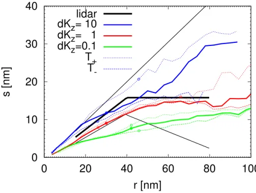
In Fig. 5 we show the mean model results for varying turbulence strength. The eddy

15

diffusion profile of the model reference case was multiplied by factors of 0.1 and 10, re-spectively. We observe that elevated turbulence also increases the slope of the curve. Furthermore, the turbulence strength defines the maximum distribution width reached. For example the reference case asymptotically approaches a width of about 15 nm, similar to the width observed by the lidar. For mean particle sizes larger than 40 nm the

20

cases with enhanced or reduced turbulence are larger or smaller than the mean width observed by the lidar. For smaller particle sizes the case with enhanced turbulence on the other hand agrees quite well to the observations. The observations with the largest distribution width compare well to the model results with the 10 times enhanced tur-bulence, but occur less often. Similarly the observations with the smallest distribution

25

(9)

ACPD

10, 3605–3625, 2010

Title Page

Tables Figures

◭ ◮

Back Close

Full Screen / Esc

Interactive Discussion included in the model, the eddy diffusion of the reference case might underestimate

the broadening of the size distribution due to vertical mixing.

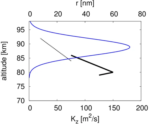
In Fig. 6 we show the eddy diffusion profile and the vertical structure of the particle size. We have extended the lidar observations of the particle size by recent measure-ments of particle sizes in PMSE (Polar Mesosphere Summer Echos) by radar (Li et al.,

5

2009). Due to the combination of strong eddy diffusion and a gradient in the particle size, turbulent mixing can increase the particle distribution width. The altitude depen-dence of eddy di_ffusion and particle size also shows a potential mechanism for an upper limit of the mean distribution width. As the turbulence strength decreases below 88 km but the particle size increases, we can expect a decrease in the broadening of

10

the distribution due to turbulence. For example the mean particle size of r=40 nm is reached at an altitude of about 84 km, where the eddy diffusion is only ∼25% of the peak value.

On the other hand we often observe a decrease of distribution width for particle sizes larger than 40 nm, especially at the lower part of the cloud. This decrease

re-15

quires another mechanism, as turbulent or wave mixing will increase the distribution width throughout the NLC layer. However, at the bottom of the layer this behavior might change. One reason could be the changing vertical gradient in the mean particle size, causing eddy diffusion to mix volumes of comparable particle sizes. Even more, particles could be mixed downward at the cloud bottom, without upward mixing from

20

below, since particles falling below the cloud bottom will evaporate. Another possible mechanism for decreasing the distribution width is that vertical winds, introduced by gravity waves, can separate small particles from the larger ones. Potentially, redistribu-tion of water to lower altitudes by freeze-drying also might shift the nuclearedistribu-tion to lower altitudes where turbulence is less active.

(10)

ACPD

10, 3605–3625, 2010

Title Page

Tables Figures

◭ ◮

Back Close

Full Screen / Esc

5 Conclusions

We have presented an extensive set of lidar observations of NLC particle properties and analyzed the dataset regarding the mean size (r) and distribution width (s). We observe a robust correlation ofs and r for mean sizes up to 40 nm. This relation is independent of the analysis method and can be found throughout the NLC layer. The

5

distribution widths can be approximated from the mean particle size by s=0.4·r. Al-lowing an accuracy of±25%, 70% of the lidar observations, analyzed with the highest possible vertical resolution, are compatible with this simple relationship. The approx-imation becomes even better if in addition a constant distribution width ofs≈15 nm is used forr≥40 nm.

10

A microphysical model of NLC (CARMA) can reproduce the observed correlation for smaller particles. We find that the slope is defined by the strength of vertical mixing due to eddy di_ffusion. A smaller fraction of observations shows a combination ofsandrthat can be explained by 10 times increased eddy diffusion. The model also reproduces that the distribution width for larger particles becomes constant. This constant distribution

15

width could be caused by the fact that we observe larger particles in the lower part of the NLC layer. At altitudes where the mean particle size is above 40 nm, the diffusion coefficient is at most 25% of the peak value of eddy diffusion.

Our investigation shows that the observed dependence of s on r is a valuable tool to adjust the microphysical processes in modeling of NLC, primarily the eddy diffusion

20

or wave mixing. The observed approximation of distribution width as function particle size is of importance for other instruments that can not directly measure the distribution width and the particle size.

Acknowledgements. We gratefully acknowledge the support of the ALOMAR staffand help-ing to accumulate the extensive data set of NLC observations. The observations were

sup-25

(11)

ACPD

10, 3605–3625, 2010

Title Page

Tables Figures

◭ ◮

Back Close

Full Screen / Esc

References

Bailey, S. M., Thomas, G. E., Rusch, D. W., Merkel, A. W., Jeppesen, C. D., Carstens, J. N., Randall, C. E., McClintock, W. E., and Russell, J. M.: Phase functions of polar mesospheric cloud ice as observed by the CIPS instrument on the AIM satellite, J. Atmos. Sol.-Terr. Phy., 71, 373–380, doi:10.1016/j.jastp.2008.09.039, 2009. 3607

5

Baumgarten, G. and Fiedler, J.: Vertical structure of particle properties and water content in noctilucent clouds, Geophys. Res. Lett., 35, L10811, doi:10.1029/2007GL033084, 2008. 3608, 3610

Baumgarten, G., L ¨ubken, F.-J., and Fricke, K. H.: First observation of one noctilucent cloud by a twin lidar in two different directions, Ann. Geophys., 20, 1863–1868, 2002,

10

http://www.ann-geophys.net/20/1863/2002/. 3609

Baumgarten, G., von Cossart, G., and Fiedler, J.: The size of noctilucent cloud particles above ALOMAR (69N,16E): optical modeling and method description, Adv. Space Res., 40(6), 772– 784, doi:10.1016/j.asr.2007.01.018, 2007. 3608

Baumgarten, G., Fiedler, J., L ¨ubken, F.-J., and von Cossart, G.: Particle properties and water

15

content of noctilucent clouds and their interannual variation, J. Geophys. Res., 113, D06 203, doi:10.1029/2007JD008884, 2008. 3607, 3609, 3618

Berger, U. and von Zahn, U.: Icy particles in the summer mesopause region: three-dimensional modeling of their environment and two-dimensional modeling of their transport, J. Geophys. Res., 107, 1366, doi:10.1029/2001JA000316, 2002. 3608

20

Fiedler, J., von Cossart, G., and Baumgarten, G.: Noctilucent clouds above ALOMAR between 1997 and 2001: occurrence and properties, J. Geophys. Res., 108, 8453, doi:10.1029/2002JD002419, 2003. 3611

Fiedler, J., Baumgarten, G., and L ¨ubken, F.-J.: NLC observations during one solar cycle above ALOMAR, J. Atmos. Sol.-Terr. Phy., 71, 424–433, doi:10.1016/j.jastp.2008.11.010, 2009.

25

3609

Fritts, D. C., Isler, J. R., Thomas, G. E., and Andreassen, Ø.: Wave breaking signatures in noctilucent clouds, Geophys. Res. Lett., 20, 2039–2042, 1993. 3607

Gadsden, M. and Schr ¨oder, W.: Noctilucent Clouds, Springer-Verlag, New York, 1989. 3606 Hervig, M., Thompson, R. E., McHugh, M., Gordley, L. L., Russel III, J. M., and Summers, M. E.:

30

(12)

ACPD

10, 3605–3625, 2010

Title Page

Tables Figures

◭ ◮

Back Close

Full Screen / Esc

Hervig, M. E., Gordley, L. L., Stevens, M. H., Russell, J. M., Bailey, S. M., and Baum-garten, G.: Interpretation of SOFIE PMC measurements: cloud identification and derivation of mass density, particle shape, and particle size, J. Atmos. Sol.-Terr. Phy., 71, 316–330, doi:10.1016/j.jastp.2008.07.009, 2009. 3610, 3611

Jensen, E. J. and Thomas, G. E.: Numerical simulations of the effects of gravity waves on

5

noctilucent clouds, J. Geophys. Res., 99, 3421–3430, doi:10.1029/93JD01736, 1994. 3609 Li, Q., Rapp, M., R ¨ottger, J., Latteck, R., Zecha, M., Strelnikova, I., Baumgarten, G., Hervig, M.,

Hall, C., and Tsutsumi, M.: Microphysical parameters of mesospheric ice clouds derived from calibrated observations of polar mesosphere summer echoes at Bragg wavelengths of 2.8 m and 30 cm, J. Geophys. Res., doi:10.1029/2009JD012271, in press, 2009. 3613, 3625

10

L ¨ubken, F.: Seasonal variation of turbulent energy dissipation rates at high latitudes as de-termined by in situ measurements of neutral density fluctuations, J. Geophys. Res., 102, 13441–13456, doi:10.1029/97JD00853, 1997. 3625

L ¨ubken, F.-J.: Thermal structure of the arctic summer mesosphere, J. Geophys. Res., 104, 9135–9149, doi:10.1029/1999JD900076, 1999. 3606

15

Rapp, M. and Thomas, G. E.: Modeling the microphysics of mesospheric ice particles: assess-ment of current capabilities and basic sensitivities, J. Atmos. Sol.-Terr. Phy., 68, 715–744, doi:10.1016/j.jastp.2005.10.015, 2006. 3608, 3609, 3612

Rapp, M., L ¨ubken, F.-J., M ¨ullemann, A., Thomas, G., and Jensen, E.: Small scale temperature variations in the vicinity of NLC: experimental and model results, J. Geophys. Res., 107,

20

4392, doi:10.1029/2001JD001241, 2002. 3609

Rapp, M., Thomas, G. E., and Baumgarten, G.: Spectral properties of mesospheric ice clouds: evidence non-spherical particles, J. Geophys. Res., 112, 3211, doi:10.1029/2006JD007322, 2007. 3609, 3611

Robert, C. E., von Savigny, C., Burrows, J. P., and Baumgarten, G.: Climatology of noctilucent

25

cloud radii and occurrence frequency using SCIAMACHY, J. Atmos. Sol.-Terr. Phy., 71, 408– 423, doi:10.1016/j.jastp.2008.10.015, 2009. 3607

Seele, C. and Hartogh, P.: Water vapor of the polar middle atmosphere: annual variation and summer mesosphere conditions as observed by ground-based microwave spectroscopy, Geophys. Res. Lett., 26, 1517–1520, doi:10.1029/1999GL900315, 1999. 3606

30

Thomas, G. E.: Solar Mesosphere Explorer measurements of polar mesospheric clouds (noc-tilucent clouds), J. Atmos. Terr. Phys., 46, 819–824, 1984. 3606

(13)

ACPD

10, 3605–3625, 2010

Title Page

Tables Figures

◭ ◮

Back Close

Full Screen / Esc

model describing aerosol formation and evolution in the stratosphere: II. Sensitivity stud-ies and comparison with observations., J. Atmos. Sci., 36, 718–736, doi:10.1175/1520-0469(1979)036<0718:AODMDA>2.0.CO;2, 1979. 3608

Turco, R. P., Hamill, P., Toon, O. B., Whitten, R. C., and Kiang, C. S.: A one-dimensional model describing aerosol formation and evolution in the stratosphere: I. Physical

pro-5

cesses and mathematical analogs, J. Atmos. Sci., 36, 699–717, doi:10.1175/1520-0469(1979)036<0699:AODMDA>2.0.CO;2, 1979. 3608

Turco, R. P., Toon, O. B., Whitten, R. C., Keesee, R. G., and Hollenbach, D.: Noctilucent clouds: simulation studies of their genesis, properties and global influences, Planet. Space Sci., 30, 1147–1181, 1982. 3609

10

von Savigny, C., Petelina, S. V., Karlsson, B., Llewellyn, E. J., Degenstein, D. A., Lloyd, N. D., and Burrows, J. P.: Vertical variation of NLC particle sizes retrieved from Odin/OSIRIS limb scattering observations, Geophys. Res. Lett., 32, L07806, doi:10.1029/2004GL021982, 2005. 3610

Witt, G.: Height, structure and displacements of noctilucent clouds, Tellus, 14, 1–18, 1962.

15

(14)

ACPD

10, 3605–3625, 2010

Title Page

Tables Figures

◭ ◮

Back Close

Full Screen / Esc

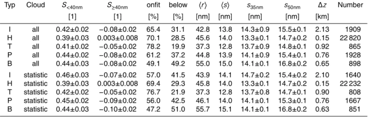
Table 1. Particle properties and slope (S) of the fit for di_fferent analysis methods/layer parts. I: vertical integral (method 3), H: highest resolution (method 1), T: NLC top, P: NLC peak, B: NLC bottom (method 2). The probability of finding particle soundings close to the fitted slope (±25%) is listed in column onfit. The probability for finding particle ensembles where the width is smaller than expected from the fit is listed in column below. hriandhsiare the mean radius and mean width, respectively.s_35nmands_50nmgive the width atr=35 nm andr=50 nm, respectively. The width of the layer is shown in column∆zand the number of measurements is found in the last column. Cloud type “all” includes all clouds observed, while “statistic” denotes clouds withβ>4×10−10m−1sr−1used for statistical studies (e.g., Baumgarten et al., 2008).

Typ Cloud S<40nm S≥40nm onfit below hri hsi s35nm s50nm ∆z Number

[1] [1] [%] [%] [nm] [nm] [nm] [nm] [km]

(15)

ACPD

10, 3605–3625, 2010

Title Page

Tables Figures

◭ ◮

Back Close

Full Screen / Esc

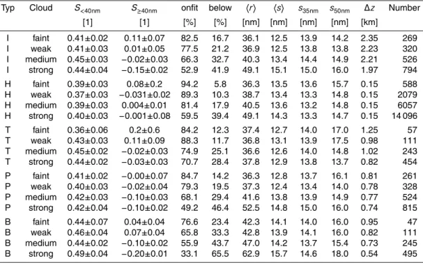
Table 2. Particle properties and slope (S) of the fit for different cloud classes and analysis methods. I: vertical integral (method 3), H: highest resolution (method 1), T: NLC top, P: NLC peak, B: NLC bottom (method 2). The probability of finding particle soundings close to the fitted slope (±25%) is listed in column onfit. The probability for finding particle ensembles where the width is smaller than expected from the fit is listed in column below. Further explanations are given in caption of Table 1.

Typ Cloud S_<_40nm S_≥_40nm onfit below hri hsi s_35nm s_50nm ∆z Number

[1] [1] [%] [%] [nm] [nm] [nm] [nm] [km]

I faint 0.41±0.02 0.11±0.07 82.5 16.7 36.1 12.5 13.9 14.2 2.35 269

I weak 0.41±0.03 0.01±0.05 77.5 21.2 36.9 12.5 13.8 13.8 2.23 320

I medium 0.45±0.03 −0.02±0.03 66.3 32.7 40.3 13.4 14.4 14.9 2.21 526

I strong 0.44±0.04 −0.15±0.02 52.9 41.9 49.1 15.1 15.0 16.0 1.97 794

H faint 0.39±0.03 0.08±0.2 94.2 5.8 36.3 13.5 13.6 15.7 0.15 588

H weak 0.37±0.03 −0.031±0.02 89.3 10.3 38.7 13.4 13.3 14.8 0.15 2079

H medium 0.39±0.03 0.004±0.01 81.4 17.9 40.5 13.6 13.2 14.8 0.15 6057

H strong 0.40±0.03 −0.001±0.08 59.5 39.4 49.1 14.3 13.3 14.7 0.15 14 096

T faint 0.36±0.06 0.2±0.6 84.2 12.3 37.4 12.7 14.0 17.0 1.25 57

T weak 0.43±0.03 0.11±0.09 88.3 11.7 36.8 13.1 13.9 17.5 0.98 111

T medium 0.45±0.02 −0.02±0.03 74.9 25.1 36.6 12.6 14.0 14.8 1.02 243

T strong 0.44±0.02 −0.03±0.03 70.7 28.4 37.8 12.9 13.8 13.7 0.82 454

P faint 0.41±0.02 −0.00±0.07 84.7 14.2 36.3 12.8 13.7 16.1 0.81 261

P weak 0.40±0.03 −0.02±0.04 79.3 19.5 37.3 12.4 13.4 14.0 0.78 328

P medium 0.42±0.03 −0.10±0.03 68.1 29.4 41.6 13.8 13.9 14.9 0.77 524

P strong 0.42±0.04 −0.10±0.02 49.2 46.4 52.5 14.8 15.0 16.0 0.74 815

B faint 0.44±0.07 0.04±0.04 76.6 23.4 42.3 14.1 14.0 16.0 0.95 47

B weak 0.46±0.04 0.07±0.04 65.8 33.3 42.8 13.9 14.1 16.0 0.82 111

B medium 0.44±0.02 −0.10±0.02 55.9 43.7 47.0 14.2 13.7 15.4 0.73 245

(16)

ACPD

10, 3605–3625, 2010

Title Page

Tables Figures

◭ ◮

Back Close

Full Screen / Esc

(17)

ACPD

10, 3605–3625, 2010

Title Page

Tables Figures

◭ ◮

Back Close

Full Screen / Esc

(18)

ACPD

10, 3605–3625, 2010

Title Page

Tables Figures

◭ ◮

Back Close

Full Screen / Esc

(19)

ACPD

10, 3605–3625, 2010

Title Page

Tables Figures

◭ ◮

Back Close

Full Screen / Esc

0

10

20

30

40

0

20

40

60

80

100 s [nm]

r [nm]

2009-12-02

t<1 day

t

≥

1 day

Fig. 4.Mean size and width of the particle size distribution at the peak of the layer for several CARMA simulations with varying temperature (reference±10 K) and H2O (reference·0.3...3)

On microphysical processes of noctilucent clouds (NLC): observations and modeling of mean and width of the particle size-distribution

ACPD

On microphysical processes of

noctilucent clouds (NLC): observations

and modeling of mean and width of the

particle size-distribution

ACPD

ACPD

ACPD

ACPD

ACPD

ACPD

ACPD

ACPD

ACPD

ACPD

ACPD

ACPD

ACPD

ACPD

ACPD

ACPD

ACPD

ACPD

0

10

20

30

40

0

20

40

60

80

100

s [nm]

r [nm]

t<1 day

t

≥

1 day

ACPD

0

10

20

30

40

0

20

40

60

80

100

s [nm]

r [nm]

lidar

dK

= 10

dK

= 1

dK

=0.1

T

T

ACPD

70

75

80

85

90

95

0

50

100

150

200

0

20

40

60

_z