On the Geometric Modeling of the Uplink Channel in a Cellular System

Journal of Engineering Science and Technology Review 1 (2008) 75- 82

Lecture Note

On the Geometric Modeling of the Uplink Channel in a Cellular System

K. B. Baltzis*

RadioCommunications Laboratory, Section of Applied and Environmental Physics,Dept. of Physics, Aristotle University of Thessaloniki, 54124, Thessaloniki, Hellas

Received 23 April 2008; Accepted 17 November 2008

___________________________________________________________________________________________

Abstract

To meet the challenges of present and future wireless communications realistic propagation models that consider both spatial and temporal channel characteristics are used. However, the complexity of the complete characterization of the wireless medium has pointed out the importance of approximate but simple approaches. The geometrically based methods are typical examples of low–complexity but adequate solutions. Geometric modeling idealizes the aforementioned wireless propagation environment via a geometric abstraction of the spatial relationships among the transmitter, the receiver, and the scatterers. The paper tries to present an efficient way to simulate mobile channels using geometrical–based stochastic scattering models. In parallel with an overview of the most commonly used propagation models, the basic principles of the method as well the main assumptions made are presented. The study is focused on three well–known proposals used for the description of the Angle–of –Arrival and Time–of–Arrival statistics of the incoming multipaths in the uplink of a cellular communication system. In order to demonstrate the characteristics of these models illustrative examples are given. The physical mechanism and motivations behind them are also included providing us with a better understanding of the physical insight of the propagation medium.

Keywords: Angle of arrival, time of arrival, scattering, geometric, cellular communications.

___________________________________________________________________________________________

J

estr

JOURNAL OF Engineering Science and

Technology Review

www.jestr.org

______________

©

1. Introduction

Telecommunication has experienced significant changes over the past few years and its paradigm has moved from wired to wireless communications. Users demand multimedia services on their mobile devices similar to the ones they have on the wired, new services are added, high data rates carry multimedia communications, and networks are asked to deal with a multimedia traffic mix of voice, data, and video, each having different transfer requirements, [1]. With the current growth of demand on wireless systems, new methods are being designed to mitigate interference and improve signal quality. Radio system engineers are asked to be able to utilize the spatial domain to enhance system performance by rejecting interfering signals and boosting desired signal levels. However the characterization of the propagation radio channel still remains a fundamental research area in wireless communications.

To meet the challenges of present and future wireless communications realistic channel models that take into account the spatial and the temporal channel characteristics must be used. A common approach is the assumption that multipath reflection is caused by scatterers located close to the mobile station (MS) targeting to the computation of the probability density function (pdf) of the Angle–of–Arrival

(AoA) and the Time–of–Arrival (ToA) of the transmitted signal. Single bounce geometrical models, i.e. models in which it is assumed that each multipath component undergoes only one bounce traveling from the transmitter to the receiver, have been deployed for the two–dimensional space providing adequate results. In these models scatterers lie in an ellipse which encompasses the transmitter and the receiver located on the foci, [2], are uniformly distributed around the mobile within either a circle, [3-5], an ellipse [5], or a hollow disc, [6], or are spatially distributed at an inverted parabolic spatial distribution on a two–dimensional disc centered at the mobile, [7]. The clustering approach, [8], which considers that signal angular spread comes from several clusters, shows a good agreement with experimental results. Two bounce geometric models, [9], show an improvement in prediction accuracy in both indoor and outdoor macrocellular environments. Proposals that involve a Gaussian, [10], or a Laplacian, [11], instead of a uniform scatterer density are also found in literature expecting to be a more appropriate candidate for modeling the realistic scattering channel. Recently, [12], a statistical scattering model based on measurements observed at the base station (BS) in an urban environment indicated that the description of the characteristics of the effective scattering area is a multivariate analysis problem, [13]. More sophisticated approaches such the one in [14] where a model for multiple– input multiple–output (MIMO) wireless propagation channels for both macro– and microcells including single and double scattering around both BS and MSs, scattering by far clusters, wave guiding, and diffraction by roof edges,

J

estr

______________

* E-mail address kmpal@physics.auth.gr

indicate the complexity of the complete characterization of the wireless channel pointing out the importance of simple approximate approaches.

Despite their complexity two–dimensional models fail to describe any signal variations in the vertical plane. However as long as the spatial correlation properties of the received signal depend on the signal angular spreading, description of vertical spreading of the waves is particularly important especially when vertical or planar arrays are used. A non– zero elevation AoA is quite common in urban areas when the propagating wave reflects off vertical structures like hills or buildings. Several researches have observed spreading of the waves in the elevation plane; see [15-16] for example. The first model that recognizes the 3–D nature of the waves spreading has been proposed thirty years ago by Aulin, [17], introducing an additional nonzero elevation angle for the incident waves. There signals arriving at the mobile were

assumed uniformly distributed within

(

0, 2

π

]

while a

particular non–uniform pdf was proposed for the elevation angle obtaining closed–form expressions of the temporal autocorrelation function and the Doppler power spectral density. However the model was characterizing from an unrealistic flatness especially at high Doppler frequencies. The problem was partially solved in [18-19] where a more realistic pdf expression for the vertical AoA was suggested while various parameters affecting the cross correlation between antennas, e.g. the direction of motion, the BS antenna height, the radius of the scattering center, and the length of the test route were used in the calculations. Unfortunately in these models the temporal autocorrelation function and the Doppler power spectral density had no more analytical solutions. An extension of these ideas was presented in [20] where a generalization of Jakes model, [21], that produces the desired spatio–temporal characteristics incorporating the ideas proposed in [17-19], takes place yielding a more realistic description but implementing far more complexity. These models assumed specific scatterers geometry while the crosscorrelation function between two sub–channels was not expressed analytically. A further development of the previous ideas is presented in [22] where the crosscorrelation function is formulated as a function of the spatial separation of antennas, time, and carrier frequencies in terms of physical channel parameters such as mobile speed, delay profile and scatterers distribution around both BS and MS providing us with a better understanding of the complicated nature of the non–isotropic propagation media. However, only if exact results are required the models complexity and the computational cost of the algorithms are worthwhile. Their direct realization in software or hardware is also extremely difficult. In any case, the outcome of a model should be interpreted taking into account the required accuracy.

This is the main reason why models such the ones presented in [23-29] have been proposed. In [23] a 3–D deterministic simulation model that takes into account both temporal and spatial channel characteristics is presented. Based on given theoretical reference models, its parameters are calculated by the Lp–norm method, [30], enabling the emulation of the received signal with any given pdf of the spatial AoA reducing complexity. A different approach is followed in [24] where the spatio–temporal characteristics of a channel in urban environment are found based on 3–D ray tracing techniques, [31]. This non statistical spatio–temporal characterization of radio channels thanks to the characteristic function of the channel can provide us with all the wideband

parameters which evaluate the coherence and dispersion properties of the radio link. However the computational cost of ray tracing techniques still remains their major drawback. Proposals in [25-26] approach the problem of spatial AoA pdf derivation differently. The mobile is assumed to be surrounded by scatterers forming a spheroid, [25], and a half–spheroid, [26], surface allowing the derivation of closed–form pdf expressions. Their simplicity makes them very useful for the performance evaluation of a wireless communication system in a macrocellular environment. A similar approach suitable for microcellular and picocellular systems is adopted in [27]. In this, scatterers are assumed to be randomly located around and between both BS and MS within a spheroid. The geometrically based elliptical model is proposed in [28] and extended in [29] for wideband multiple–input multiple–output (MIMO) channels allowing the derivation of analytical expressions for the 3–D space– time cross–correlation, temporal autocorrelation and frequency correlation functions.

In this paper a brief introduction in the basic principles of geometric modeling and its application in the characterization of the wireless propagation medium are given. The main objective of the paper is the presentation of the key ideas of the method accompanying with illustrative examples that exhibit the characteristics, advantages, and potential applications of the method. The study is focused on three characteristic proposals used for the description of macro– and microcellular wireless systems in the two and three dimensions. Owning to text size limitation we will examine the reverse link only, however similar approaches may be used in the downlink also. The paper is organized as follows: In the next Section the basic principles and assumptions of geometrical modeling are presented. In Section III three well–known geometric models, the 2–D Geometrical–Based Single Bounce Macrocellular (2–D GBSBM), [3-5], also known as circular scattering model, the elliptical scattering model, [5], and the 3–D spheroid model, [25], are extensively described. Results and discussions are provided in Section IV. Finally, Section V concludes the paper.

2. Geometric Modeling: Basic Principles and Assum-ptions

Derivation of the geometric models is based on a serious of assumptions. Based on the assumptions made the models can be used for macro–, micro–, or picocellular systems, for environments with various BS and MS antenna heights, and for narrowband or wideband systems, see [26], [32-33] for details. Common assumptions refer to the shape of the scatterers region, their density function within it, the number of scatterers each propagation path between the mobile and the base station reflects of with the influence of others assumed to be negligible, and the BSs and MSs antennas directivity patterns, [34], and heights. A few more common assumptions imply that each scatterer behaves as an omni– directional lossless reradiating element, independent of other scatterers, or refer to the scattering coefficients values and their phases. For simplicity polarization effects are usually overlooked.

3. The Circular, the Elliptical and the Spheroid Model: Three Typical Geometrical – based Scattering Approaches

In this Section an analytical description of the characteristics and the mathematical formulation of three well–known geometrical–based scattering models, the circular, the elliptical, and the spheroid one, that describe the statistics of the AoA of the multipath signals at the base station are presented. The elliptical model describes also the statistics of the ToA. The first two models describe signal variations in the azimuthal plane only. In the spheroid model both azimuthal and elevation coordinates are considered.

Circular model:

The circular model, [3-5], also known as 2–D GBSBM is probably the simplest two–dimensional geometrical–based statistical single bounce model. It considers the scatterers uniformly distributed within a circle of radius

R

around the mobile unit. The signals received at the base station are assumed to be plane waves arriving from the horizon, and hence the AoA calculation includes only the azimuthal coordinate. It also considers that these signals have interacted with only one scatterer in the channel with the influence of others assumed to be negligible (single bounce model). Also the mobile antennas radiation patterns are omni–directional and the scatterers are assigned equal scattering coefficients with uniform random phases. Under these assumptions the model is suitable for macrocell environments where antenna heights are relatively large, [32].

The model is illustrated in Fig. 1. The base station, marked as BS, and the mobile station, marked as MS, are separated by a distance

D

. The location of each scatterer is marked as S. Although only one scatterer is shown in the figure, it is considered that there are many of them uniformly distributed within the scattering circle.

R

>

In this model the pdf of the AoA of the multipath

components

f

_c

( )

φ

is calculated as the derivative of the

corresponding cumulative distribution function (cdf),

( )

c

F

φ

. Since the scatterers are uniformly distributed within the scattering circle the area within the shaded region is proportional of the AoA of the multipath components. As

a result

F

_c

( )

φ

equals to the area of the shaded region, see

Fig. 1, multiplied by the scatterers density within the circle, i.e.:

( )

22 12

0

d

2

c area

r

r

F

f

φ

φ

=

_∫

−

β

(1)

Fig. 1. Geometrical configuration of the circular (2–D GBSBM)

here and are given by

channel model.

w

r

₁

r

₂

( )

( )

2 2 2

cos 1i sin , 1, 2

i i

r ≡r β =D β+ − ∓ R −D β i= (2)

hile the scatterers density is w

2

1

area

f

R

π

=

(3)

The pdf of the AoA is the derivative of the cdf with respect to

φ

. From (1)-(3) comes that

( )

( )

2 2

( )

(

)

max

2

cos 1 sin

c

D D

f

R R

φ φ φ φ φ

π ⎛ ⎞

= −_{⎜ ⎟} ⋅Π

⎝ ⎠ − (4)

where

Π

( )

x

is the unit step function and

φ

_max is (due to

fineme cle

the con nt of the scatterers within a cir around the mobile) the maximum AoA of a multipath component at the BS given by:

(

)

1 max

sin

R D

φ

₌

−

(5)

The model predicts a relatively high probability of

3

lliptical model:

about 100–200 wavelengths for 900 MHz, which provides a range of 30–60 m, roughly the width of wide urban streets.

E

iptical model, [5], are similar The assumptions used in the ell

to these the circular model uses with the exception that scatterers are uniformly distributed inside an ellipse with foci at the base station and the mobile unit, see Fig. 2.

BS

MS

D

B

A

S

y

x

φ

Fig. 2. The Geometrical Based Ellip cal Model.

The axes of the ellipse are

ti

2

A

=

c

τ

m (6)

2 2 2

2

B

=

c

τ

_m

−

D

(7)

here is the speed of light,

w

c

τ

_m is the maximum delay

he spread associated with scatterers within the ellipse, and

D

is the BS to MS distance. The equations that describe t ellipse with respect to the BS position are respectively in Cartesian and polar coordinates the:

2 2

2

1

x

D

y

A

B

−

⎛

⎞

₊

⎛ ⎞

₌

⎜

⎟

⎜ ⎟

⎝

⎠

⎝ ⎠

(8)

(

)

2

2

2

cos

r

=

B

A D

−

φ

(9)

The model is appropriate for wideband microcell environments where antenna heights are relatively low, [5], [32]. It has the physical interpretation that only multipath components that arrive with a maximum delay of

τ

_m are

accounted for while the ones with longer delays are ignored since they experience greater path loss, and hence have relatively low power compared to those with shorter delays. Provided that

τ

_m is properly chosen, the model may account

for nearly all the power and AoA of the incoming multipaths. Its choice determines both the angle and the delay spread of the channel. Various methods for selecting an appropriate value of

τ

_m can be found in literature, see [2]

for example. The assump n of antennas with low heights allows the consideration that the BS may receive multipath reflections from locations near both itself and the MS. The model can be used for both the reverse and the forward link.

However in this paper only the first case will be presented, see [5] for the forward case.

In the model the joint AoA/ToA pdf is calculated as a function of the angle

φ

and the delay

τ

. The formulation used is based on the calculation of the Jacobian determinants, [37], that describe the transformation of the polar to rectangular coordinates and vice versa. It comes, [5], that the uplink joint AoA/ToA, marginal AoA, and marginal ToA pdfs are respectively

( )

(

)

( ) ( )

2 2 2 2 2 2 3 2 cos ,

cos

m

e m

m

c D c D Dc D

f

c

c D

τ τ τ φ

φ τ τ

πτ τ φ

− + − _{⎛ ⎞}

τ τ

= ⋅Π_⎜ − _⎟⋅Π −

⎝ ⎠

−

(10)

( )

(

)

(

)

3 2 2 2 2

2

2 c

m e

m m c D f

c c D

φ _φ τ

os

π τ τ φ

− =

−

(11)

( )

(

)

(

)

2 2 2 4 2 2 4 2 2 2 2

2

e m

m m m

c D D

f

c c D c D

τ _τ τ _{τ τ}

τ τ τ τ τ

− ⎛ ⎞ _τ

= ⋅Π_⎜ − _⎟⋅Π −

⎝ ⎠

+ − +

(12)

Spheroid model:

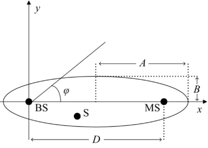
The models already presented assume an azimuthal wave spreading only. However this assumption is sometimes far from reality. A commonly used 3–D model is the spheroid, [25], used for the description of the AoA of the incoming multipaths in both BS and MS in a macrocellular environment when the MS antenna height is low compared to the BS one and multipath components can arrive from both horizontal and vertical directions to the receiving antennas.

n the spheroid model, see Fig. 3, scatterers are distributed uniformly around the MS within a half–spheroid region with semi–axes lengths

a

and

b

. The MS is located at the center of the spheroid at a distance

D

from the BS. Its antenna is assumed to be located at ground level for simplicity. The BS antenna height is

h

.

tio

)

The model can be used in both links. In this paper only the reverse case will be presented (see [25] for the forward link). The uplink joint pdf is primarily expressed in terms of

the spherical coordinates

(

r

, ,

φ θ

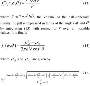
of each point of the

spheroid with respect to the BS. Derivation of pdf uses the Jacobian of the transformations between the volume differential in the Cartesian and the spherical coordinates system, see [25], [37]. It is

(

)

2

0

cos

, ,

s

r

f

r

V

θ

φ θ

=

(13)

where

V

=

2

π

a b

2

3

the volume of the half–spheroid. Finally the pdf is expressed in terms of the angles

φ

and

θ

by integrating (13) with respect to

r

over all possible values. It is finally:

( )

32 31

2 2

,

2

cos

b b

s

f

a b

ρ

ρ

φ θ

π

θ

−

=

(14)

where

ρ

_b1 and

ρ

_b2 are given by

2

2 2 2

2 2 2

2 2 2

1 2

2 2

2

cos tan cos tan 1 tan 1 tan

b b

a h a h a a h

D D D a

b b b

a b

φ θ φ θ θ

ρ

θ

⎛ ⎞ ⎛ ⎞⎛

+ ⎜ + ⎟− +⎜ ⎟⎜ −

⎝ ⎠ ⎝ ⎠⎝

=

+

∓ 222

b

⎞ + ⎟ ⎠

(15)

Integration of (14) with respect to

θ

and

φ

gives the marginal pdfs at the azimuth and the elevation plane correspondingly. These are expressed as:

( )

2 2

(

1

(

)

2

3

cos 1 sin sin

4 s

D D

f

a a

φ _{φ = φ}⎛ _{− φ}⎞_⋅Π − _−φ

⎜ ⎟

⎝ ⎠ a D

)

(16)

and

( )

(

3 3

)

2 2

2 2

1

2

cos

M

M

s b b

f

d

a b

φ θ

φ

θ

ρ

ρ

π

θ

₋

=

_∫

−

φ

(17)

where

2 2 2

1 2 2 2

2 2 2

1

cos tan 1 tan

M

a a a

h D a h

D b b b

φ ₌ −_⎜⎛ _{⋅ −}⎡_⎢ θ₊ ⎛ _{− +} ⎞⎛ ₊ ⎤_⎥⎞_⎟

⎜ ⎟⎜

⎜ ⎢_⎣ ⎝ ⎠⎝ ⎥_⎦⎟

⎝ ⎠

2θ⎞

⎟ ⎠

(18)

4. Numerical Results and Discussions

Due to scattering, multipath components arrive at different angles from those of the direct one. A common measure of the channel angular dispersion is the AoA of the multipath components. Using the models previously described we can easily calculate the uplink angular spread as well the time spread and extract a series of useful conclusions.

Fig. 4 shows the pdf of AoA of the incoming multipaths at the BS as predicted from the circular model for some sample values of BS to MS distances normalized to the radius of the scatterers disc. Notice that the pdf is an even function, as expected from (4), maximized at

φ

=

0

, and

lies between

±

φ

_max . Decrease in

D R

flattens the pdf curve. The pdfs presented here can be used to simulate a power delay profile (PDA) and to quantify angle spread for a given

D R

ratio, [4].

-15 -10 -5 0 5 10 15

0 2 4 6 8 10 12 14

f c

(

φ

)

φ(deg)

D = 20R D = 10R D = 5R

Fig. 4. Circular model: Illustration of the pdf

f

_c

( )

φ

of AoA of the incoming multipaths at the BS.

In Fig. 5 the maximum AoA of a multipath component in the azimuthal plane

φ

_max versus ratio D R is presented. The maximum angular spread

Δ

φ

in the azimuthal plane is twice the

φ

_max as expected from (4). Only for small normalized BS to MS distances (mobile close to the BS or extended scatterers region) the angular spread takes noticeable values. An increase in D R decreases the value of

φ

_max as expected from the system geometry. This dependence is almost linearly for great values of D R. In the plotted examples in Fig. 4, it is

( ) {

deg

}

φ

5

Δ

=

.7,11.5, 23.1

for

D R

=

{

20,10, 5

}

4 8 12 16 20

0 5 10 15 20 25 30 35

φ max

(d

eg

)

D / R

Fig. 5. Circular model: The maximum AoA of a multipath component at the BS versus D R.

5

μ

sec

m

τ

=

. Using (6) and (7) the semi–axes of the scattering ellipse are found

A

=

750m

and

B

=

558m

. Note that the joint pdf takes significant values for small spreading angles and time delays and is symmetric with respect to

φ

=

0

. A significant difference between the elliptical and the circular model is that the joint pdf is not maximized at

φ

=

0

(which responds to the axis that connects BS and MS) but in a small angular distance close to it. Also incoming multipaths reaches the BS from any angle

in the range

[

−

π π

,

]

.

Fig. 6. Elliptical model: Uplink joint AoA/ToA pdf.

The last comment is easily derived from Fig. 7 where the

marginal pdf

f

_eφ

( )

φ

of AoA of the incoming multipaths

at the BS is illustrated for some sample values of

D

τ

_m.

The curves are symmetric with respect to

φ

=

0

. Decrease in

D

τ

_m flattens the pdf curve and lowers the value it takes

at angles close to the LOS direction. This means that when the mobile approaches the base station or the maximum delay increases contribution of incoming multipaths of great angles increase. On the contrary when the distance between BS and MS increases or

τ

_m decreases the performance of the elliptical model approaches the circular one. It easily comes from (6) and (7) that the as the area of the ellipse decreases contribution of the incoming multipaths tends to

be uniform

∀ ∈ −

φ

[

π π

,

]

.

In Fig. 8 the he marginal pdf

f

_eτ

(

φ

)

of ToA of the

incoming multipaths at the BS is illustrated for some sample values of

D

and

τ

_m. The plot shows that there is a high

density of scatterers with relatively small delays (obviously it is always

τ

≥

D c

and

τ τ

≤

_m

( )

). Similarities are easily found between the curves. It can easily be proven by differentiating (12) that

arg min

f

e

3

D

2

c

τ

τ

τ

=

, a

value that depends on the distance between the BS and the MS only and not on the maximum delay spread, or in other

words, only on the system geometry and not on the propagation characteristics, a significant conclusion for receivers design.

-150 -100 -50 0 50 100 150 0.00

0.25 0.50 0.75 1.00 1.25 1.50

f

φ

e

(

φ

)

φ(deg)

D/τ_m=c/10 D/τ_m=3c/10 D/τ_m=5c/10 D/τ_m=2c/3 D/τ_m=7c/10 D/τ_m=9c/10

Fig. 7. Elliptical model: Marginal pdf

f

_eφ

( )

φ

of AoA of the incoming multipaths at the BS.

1 2 3 4 5 6 7 8 9 1

0.00 0.25 0.50 0.75 1.00

0 D=500m

f

τ (φ_e

)

τ(μsec)

τm=5μsec

τm=10μsec

D=1000m

Fig. 8. Elliptical model: Marginal pdf

f

_eτ

( )

φ

of AoA of the

incoming multipaths at the BS for various

D

and

τ

_m.

Fig. 9 shows the contour plot of the normalized joint pdf that the 3–D spheroid model predicts for a wireless system with

h

= =

a

D

2

. In order to lower the computational cost it has been considered that

b

. It is noticed that the incoming multipaths at the BS from the semicircle of the scattering disc closer to the BS have lower pdf values. In the azimuth plane the pdf has a maximum at

a

0

φ

=

and is symmetric with respect to it. In the elevation plane the joint

pdf has its maximum at , while

(

o 0

20

θ

≅

o

26.6

θ

_BS-MS

=

(

)

1 BS-MS cot D h

θ

₌ − _{, the angle that points to the MS). A}

series of simulations performed have shown that in any case it is

( )

( )

1

(

arg max f_s 0, arg maxf_sθ cot

)

θ

θ

θ

θ

−

< < D h (19)

from the conical projections with tip the desired BS and

angles

θ

,

φ

,

θ

+ Δ

θ

, and

φ

+ Δ

φ

as

θ

increases. This remark may be quite useful in applications such as beamforming or location estimation systems, see [38-39] for example.

Fig. 9. Spheroid model: Contour plot of the normalized joint pdf of the AoA of the incoming multipaths at the BS (

h

= =

a

D

2

).

Fig. 10 shows some sample pdfs in the azimuth plane for the spheroid and the circular models (it has been set

R

≡

a

). In both models, the depth of scatterers (extent of the scattering region along radial lines from the origin)

decreases as

φ

increases. However, the scatter region for

the spheroid model has maximum height along

φ

=

0

and zero height along

φ φ

=

_max

0

. Because of the combined effects of depth and height, contribution from off–axis scatterers (i.e., from

φ

≠

) is different for the spheroid model compared to the 2–D GBSBM.

Fig. 10. Pdf of the AoA of the incoming multipaths in the azimuthal plane as seen at the BS: Comparison between spheroid and circular models.

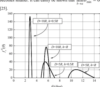
The elevation plane marginal pdf was evaluated by assuming that

b

. The results are plotted in Fig. 11 for various system geometries. Note that as the BS to MS distance increases or the BS antenna height decreases

angular spreading takes smaller values. In this case also, the

range of values

a

( )

s

f

θ

θ

is non–zero approaches the

0

θ

=

. These conclusions are easily drawn from the system geometry. It has to be mentioned that for comparable values of and curves are similar to these illustrated in Fig. 11 but the angle spreading is greater. As

b

increases the

minimum value of

a

b

θ

for which

f

_sθ

( )

θ

≠

0

,

θ

_min , becomes smaller. It can easily be shown that

li

m

_min

0

b→a

θ

=

,

[25].

0 2 4 6 8 10 12 14

0 20 40 60 80 100 120 140 160

D=10R, h=0.5R

D=5R, h=0.5R _{D=5R, h=R}

θ

fs

(

θ

)

D

θ (deg)

=10R, h=R

Fig. 11. Spheroid model: Marginal pdf of the AoA of the incoming multipaths in the elevation plane as seen at the BS for various system geometries.

5. Conclusions

An overview of the basic principles of geometric modeling has been presented in this paper. This modeling approach is useful for general system performance analysis and simultaneously provides radio engineers with a better understanding of the propagation medium. A brief review of a number of spatial propagation channels has been presented. The study has been focused in the description of three typical geometrical–based stochastic models, the circular, the elliptical, and the spheroid one, used for the description of the AoA and ToA statistics of the uplink multipaths in a cellular system. In brief the first two are 2–D models while the third one describes signal variations in both azimuthal and elevation planes. These models are interesting proposals providing us with adequate results in macrocellular, the circular and the spheroid model, and microcellular, the elliptical one, wireless communication systems. Illustrative examples have been provided exhibiting the characteristics of each model. Armed with improved spatial channel modeling tools and a greater understanding of signal propagation, engineers can begin to meet the challenges inherent in designing future high–capacity/high– quality wireless communication systems, including the effective use of smart antennas.

______________________________ References

[1] W. Webb, Wireless Communications: The Future, John Wiley & Sons Ltd., Chichester (2007).

[2] J. C Liberti and T. S. Rappaport, A geometrically based model for line-of-sight multipath radio channels, Proc. of the IEEE 46th Vehicular Technology Conference, Atlanta, USA, pp. 844–848 (1996).

[3] P. Petrus, J. H. Reed, and T. S. Rappaport, Geometrically based statistical channel model for macrocellular mobile environments, Proc. IEEE GLOBECOM’96 2, London, England, pp. 1197-1201 (1996).

[4] P. Petrus, J. H. Reed and T. S. Rappaport, Geometrical-Based Statistical Macrocell Channel Model for Mobile Environments, IEEE Trans. Commun. 50, pp. 495–502 (2002).

[5] R. B. Ertel and J. H. Reed, Angle and time of arrival statistics for circular and elliptical scattering models, IEEE J. Select. Areas Commun. 17, pp. 1829-1840 (1999).

[6] A. Y. Olenko, K. T. Wong, and E. H. -O. Ng, Analytically derived ToA-DoA statistics of uplink/downlink wireless multipaths arisen from scatterers on a hollow-disc around the mobile, IEEE Antennas Wireless Propagat. Lett. 2, pp. 345-348 (2003).

[7] A. Y. Olenko, K. T. Wong, and M. Abdulla, Analytically derived ToA-DoA statistics of uplink/downlink wireless-cellular multipaths arisen from scatterers with an inverted-parabolic spatial distribution around the mobile, IEEE Signal Processing Lett. 12, pp. 516-519 (2005).

[8] M. R. Arias and B. Mandersson, Clustering approach for geometrically based channel models in urban environments, IEEE Antennas Wireless Propagat. Lett. 5, pp. 290-293 (2006). [9] M. Mavrommatis, A. Kalis, A., and M. Carras, Two bounce

geometric model for SIR evaluation in ad-hoc networks using directional antennas, Proc. of the IEEE 16th _{International} Symposium on Personal, Indoor and Mobile Radio Communications, Berlin, Germany, pp. 501-506 (2005). [10] R. Janaswamy, Angle and time of arrival statistics for the

Gaussian scatter density model, IEEE Trans. Wireless Commun. 1, pp. 488-497 (2002).

[11] B. T. Sieskul and S. Jitapunkul, Towards Laplacian angle deviation model for spatially distributed source localization, Proc. of the International Symposium on Communications and Information Technology 1, pp. 242-247 (2004).

[12] T. Imai and T. Taga, Statistical scattering model in urban propagation environment, IEEE Trans. Veh. Technol 55, pp. 1081-1093 (2006).

[13] R. A. Johnson and D. W. Wichern, Applied Multivariate Statistical Analysis, 6th _{ed., Prentice-Hall, Englewood Cliffs} (2007).

[14] A. F. Molisch, A generic model for MIMO wireless propagation channels in macro- and microcells, IEEE Trans. Signal Process. 52, pp. 61-71 (2004).

[15] J. Fuhl, J. –P. Rossi, and E. Bonek, High resolution 3D direction of arrival determination for urban mobile radio, IEEE Trans. Antennas Propagat. 45, pp. 672-682 (1997).

[16] A. Kuchar, J. –P. Rossi, and E. Bonek, Directional macrocell channel characterization from urban measurements, IEEE Trans. Antennas Propagat. 48, pp. 137-146 (2000).

[17] T. Aulin, A modified model for the fading signal at a mobile radio channel, IEEE Trans. Veh. Technol. 28, pp. 182-202 (1979).

[18] J. D. Parsons and A. M. D. Turkmani, Characterisation of mobile radio signals: Model description, Proceedings IEE I-138, pp. 549-556 (1991).

[19] J. D. Parsons and M. D. Turkmami, Characterisation of mobile radio signals: Base station crosscorrelation, Proceedings IEE I-138, pp. 557-565 (1991).

[20] Y. Z. Mohasseb and M. P. Fitz, A 3–D spatio–temporal simulation model for wireless channels, IEEE J. Select. Areas Commun. 20, pp. 1193-1203 (2002).

[21] W. C. Jakes, Microwave Mobile Communications, 2nd _{rev. ed.} Wiley-IEEE Press, New York (1994).

[22] H. S. Rad and S. Gazor, A 3D correlation model for MIMO non– isotropic scattering with arbitrary antenna arrays, Proc. IEEE Wireless Communications and Networking Conference 2, New Orleans, USA, pp. 938-943 (2005).

[23] Q. Yao and M. Pätzold, A novel 3–D spatial–temporal deterministic simulation model for mobile fading channels, Proc. of the IEEE 14th _{International Symposium on Personal, Indoor} and Mobile Radio Communications 2, Beijing, China, pp. 1506-1510 (2003).

[24] Y. Chartois, Y. Pousset, and R. Vauzelle, A spatio–temporal radio channel characterization with a 3D ray tracing propagation model in urban environment, Proc. of the IEEE 15th _{International} Symposium on Personal, Indoor and Mobile Radio Communications 4, Barcelona, Spain, pp. 2431-2435 (2004). [25] R. Janaswamy, Angle of arrival statistic for a 3–D spheroid

model, IEEE Trans. Veh. Technol. 51, pp. 1242-1247 (2002). [26] A. Y. Olenko, K. T. Wong, S. A. Oasmi, and J. Ahmadi–

Shokouth, Analytically derived uplink/downlink TOA and 2-D-DOA distributions with scatterers in a 3-D hemispheroid surrounding the mobile, IEEE Trans. Antennas Propagat. 54, pp. 2446-2454 (2006).

[27] M. Alsehaili, A. R. Sebak, and S. Noghanian, An improved 3D geometric scattering channel model for wireless communications, Proc. 2007 URSI EMTS Commission B – Electromagnetic Theory Symposium, Ottawa, Canada, (2007).

[28] M. Pätzold and N. Youssef, Modelling and simulation of direction–selective and frequency–selective mobile radio channels, AEU – International Journal of Electronics and Communications 55, pp. 433-442 (2001).

[29] M. Pätzold and B. O. Hogstad, A wideband MIMO channel model derived from the geometric elliptical scattering model, Wireless Communications and Mobile Computing (in press). DOI: 10.1002/wcm.572 (2007).

[30] M. Pätzold, Mobile Fading Channels, John Wiley & Sons, Ltd., Chichester (2002).

[31] P. A. Bello, Characterization of randomly time–variant linear channels, IEEE Trans. on Commun. 11, pp. 360-393 (1963). [32] R. B. Ertel, P. Cardieri, K. W. Sowerby, T. S. Rappaport, and J.

H. Reed, Overview of spatial channel models for antenna array communication systems, IEEE Pers. Commun. 5, pp. 10-22 (1998).

[33] M. T. Simsim, Geometry-Based Stochastic Physical Channel Modeling for Cellular Environments, PhD Thesis, University of New South Wales (2006).

[34] C. A. Balanis, Antenna Theory: Analysis and Design, 3rd _ed., John Willey & Sons, Inc., Hoboken (2005).

[35] D. Aszetly, On Antenna Arrays in Mobile Communication Systems: Fast Fading and GSM Base Station Receiver Algorithms, PhD Thesis, Royal Institute of Technology (1996) [36] W. C. Y. Lee, Mobile Communications Engineering, 2nd _ed.,

McGraw-Hill, New York (1998)

[37] A. Jeffrey and H. –H. Dai, Handbook of Mathematical Formulas and Integrals, 4th _{ed., Elsevier Inc., Burlington (2008).}

[38] L. C. Godara, Smart Antennas, CRC Press LLC, Boca Raton (2004).