www.hydrol-earth-syst-sci.net/11/1405/2007/ © Author(s) 2007. This work is licensed under a Creative Commons License.
Earth System
Sciences
A conceptual investigation of process controls upon flood frequency:
role of thresholds
I. Struthers1and M. Sivapalan2,3
1School of Environmental Systems Engineering, The University of Western Australia, 35 Stirling Highway, Crawley WA
6009, Australia
2Centre for Water Research, The University of Western Australia, 35 Stirling Highway, Crawley WA 6009, Australia 3now at: Department of Geography and Department of Civil & Environmental Engineering University of Illinois at
Urbana-Champaign, Urbana, Illinois, IL 61801, USA
Received: 11 October 2006 – Published in Hydrol. Earth Syst. Sci. Discuss.: 26 October 2006 Revised: 15 May 2007 – Accepted: 8 June 2007 – Published: 6 July 2007
Abstract. Traditional statistical approaches to flood fre-quency inherently assume homogeneity and stationarity in the flood generation process. This study illustrates the impact of heterogeneity associated with threshold non-linearities in the storage-discharge relationship associated with the rainfall-runoff process upon flood frequency behaviour. For a simplified, non-threshold (i.e. homogeneous) scenario, flood frequency can be characterised in terms of rainfall frequency, the characteristic response time of the catchment, and storm intermittency, modified by the relative strength of evapora-tion. The flood frequency curve is then a consistent transfor-mation of the rainfall frequency curve, and could be readily described by traditional statistical methods. The introduction of storage thresholds, namely a field capacity storage and a catchment storage capacity, however, results in different flood frequency “regions” associated with distinctly differ-ent rainfall-runoff response behaviour and differdiffer-ent process controls. The return period associated with the transition be-tween these regions is directly related to the frequency of threshold exceedence. Where threshold exceedence is rela-tively rare, statistical extrapolation of flood frequency on the basis of short historical flood records risks ignoring this het-erogeneity, and therefore significantly underestimating the magnitude of extreme flood peaks.
1 Introduction
Flood frequency analysis is concerned with describing the probabilistic behaviour of flood peaks for a given location; specifically, it attempts to quantify the likelihood of a flood
Correspondence to:M. Sivapalan ([email protected])
of a given magnitude occurring within a given time inter-val (Pattison et al., 1977). An understanding of flood fre-quency is of direct applicability for flood forecasting, but is most commonly used for engineering design against risk; for the design of flood-managing structures, such as reservoirs, drainage systems and levees, as well as flood-impacted struc-tures, such as roads, bridges and buildings.
Less attention has been given to an examination of the im-pact of heterogeneity upon altering flood frequency. Hetero-geneity is most commonly associated with a multiplicity of mechanisms responsible for a flood peak, whether these re-late to heterogeneity in rainfall generation, or in the trans-formation of rainfall into a flood peak. Merz and Bl¨oschl (2003) identified different storm types as resulting in dif-ferent flood responses, with difdif-ferent storm types being im-portant in describing different ranges of return period within the flood frequency curve. The consequence of heterogene-ity is that, while the flood frequency curve does not vary with time, the flood frequency curve consists of different “regions” associated with different mechanisms or combina-tions of mechanisms that cannot be readily fitted by a sim-ple probability distribution function. Where heterogeneity or non-stationarity is significant, therefore, traditional statistical methods for flood frequency analysis are unsuited.
An alternative, derived flood frequency approach attempts to apply our understanding of rainfall generation behaviour, and of the transformation process from rainfall into flood response, in order to understand the dynamics of flood fre-quency and its process controls (e.g. Eagleson, 1972). Un-like statistical methods, an understanding of process con-trols upon flood frequency permits theforecastingof flood frequency subject to non-stationarity and heterogeneity, as well as a rationalisation of non-stationarity and heterogene-ity in historic flood frequency behaviour – at least qualita-tively, if not quantitatively. The objective of this study is to present an analysis of the process controls on flood frequency for a simplified representation of catchment hydrological re-sponse, and then to illustrate the impact of heterogeneity in the hydrological response – specifically, that associated with threshold non-linearities in the catchment storage-discharge relationship – in altering flood frequency behaviour. The im-pacts of specific elements of spatial and temporal variability upon flood frequency are then considered. While Kusumas-tuti et al. (2006) considers the sensitivity of flood frequency to threshold impacts for a specific climate using similar cli-mate and catchment parameterisations, this study aims to describe climate and catchment process controls upon flood frequency more generally, and to identify important param-eter groupings that can be used to generally characterise the flood frequency response, including heterogeneity therein, of a given climate-catchment combination.
2 Methodology
This study couples a stochastic rainfall generator with a spatially-lumped rainfall-runoff model, which are run con-tinuously for 1000 years in order to obtain estimates of flood frequency based on the maximum hourly flood intensity in each individual year of simulation (i.e. annual maxima se-ries). Attenuation due to runoff routing in the river network is not explicitly considered. Our analysis employs
“essen-tial” models, which contain only the basic elements of cli-mate forcing and catchment hydrological response; evapora-tion is essentially continuous, except during rainfall, while the essential properties of rainfall are its intermittency and its stochasticity. The fundamental “action” of the catchment is to facilitate attenuation and loss, giving rise to a flood re-sponse signal which is filtered relative to the rainfall forcing signal. The various simplifications employed in this study make this methodology unsuitable for accurate flood predic-tion, but have the over-riding benefit – given the study ob-jectives – of permitting the derivation of a relatively clear explanatory framework for the resulting flood frequency be-haviour in terms of dominant climate and landscape proper-ties.
2.1 Stochastic rainfall generator
Flood frequency is stochastic by its nature; in the absence of substantial historical precipitation records, the use of a stochastic rainfall generator is therefore logical for flood fre-quency examination. This study employs an event-based rainfall model similar to that of Robinson and Sivapalan (1997). In an event-based model, each “event” consists of a storm period of duration tr and average rainfall intensity
iand an inter-storm period of durationtb. While Robinson and Sivapalan (1997) considered storm intensity to be corre-lated to storm duration, in this study each of these properties is considered to be an independent, exponentially-distributed random variable, such that:
fX x| ˆx=
1 ˆ
x exp
−x ˆ
x
(1) wherexis the storm property variable (tr,i, ortb), andxˆis an average value for that variable, and noting thatE[x] terms in certain figures and expressions are equivalent toxˆ. Within-storm patterns in rainfall intensity for a given Within-storm are gen-erated using a stochastic disaggregation method, with identi-cal parameterisation and methodology as given in Robinson and Sivapalan (1997). Seasonality in storm properties is ini-tially ignored.
2.2 Conceptual catchment model
The catchment is represented as a single bucket (e.g. Man-abe, 1969) of total storage capacity, Sb, and field capacity storage,Sf c. At storages above field capacity the subsurface flow rate is linearly related to catchment storage, modulated by a characteristic response time,tc, such that:
qss(t )=
(S(t )−S
f c
tc S (t ) > Sf c
0 S (t )≤Sf c
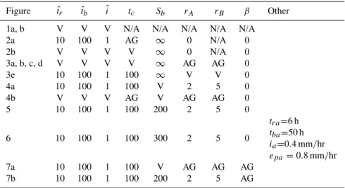
Table 1.Parameter values used in the construction of figures. V indicates parameters which can be freely varied. AG indicates parameters that vary “as given” in the legend between individual curves, and N/A indicates variables which are not applicable to the particular figure.
Figure tˆr tˆb ˆi tc Sb rA rB β Other
1a, b V V V N/A N/A N/A N/A N/A
2a 10 100 1 AG ∞ 0 N/A 0
2b V V V V ∞ 0 N/A 0
3a, b, c, d V V V V ∞ AG AG 0
3e 10 100 1 100 ∞ V V 0
4a 10 100 1 100 V 2 5 0
4b V V V AG V AG AG 0
5 10 100 1 100 200 2 5 0
6 10 100 1 100 300 2 5 0
tra=6 h tba=50 h ia=0.4 mm/hr epa=0.8 mm/hr
7a 10 100 1 100 V AG AG AG
7b 10 100 1 100 200 2 5 AG
During a storm event, evaporation is considered to be neg-ligible, with rainfall infiltration constrained only by the stor-age capacity of the catchment. When the catchment is full, surface runoff occurs at a rate equal to the rainfall rate minus the ongoing subsurface flow rate;
qs(t )=
max [i (t )−qss(t ) ,0]S (t )=Sb
0 S < Sb (3)
Thus, the equation for the rate of change of storage during a storm event is:
dS (t )
dt =i (t )−qss(t )−qs(t ) (4)
So long as storages are above field capacity, subsurface flow is continuous during the inter-storm period, while surface runoff will cease. Evaporation is considered to occur during the inter-storm period at potential rates for storages greater than field capacity, and at a linearly-reduced rate below field capacity;
e (t )=
(
ep(t ) S (t )≥Sf c
ep(t )S(t )S
f c S (t ) < Sf c
(5)
such that the rate of change of storage during the inter-storm period can be expressed as:
dS (t )
dt = −e (t )−qss(t ) (6)
Unlike storm properties, the potential evaporation rate is not considered to be stochastically variable; seasonality inepis also initially ignored, such that the value is constant during all interstorm periods.
3 Results and discussion
In attempting to summarise modelled flood frequency be-haviour, it is useful to consider certain “end-member” lim-iting cases, the behaviour of which is in some ways simpli-fied relative to the full complexity of the response. A triv-ial end-member is the case where storage is always below field capacity, such that no flood response occurs; obviously this case is of no consequence for flood frequency modelling. Two more meaningful end-member cases will be considered in turn: (i) Case 1 (maximum): an impervious catchment (i.e.Sb=0), for which all rainfall is transformed into surface runoff, and (ii) Case 2 (baseline): attenuation without thresh-olds; specifically, a deep soil with no evaporation, such that storage is always greater than field capacity but less than the total storage capacity, for which subsurface runoff will be continuously produced. Each of these end-member cases are themselves homogeneous; once these homogeneous cases are understood, we can then generalise to consider hetero-geneity associated with evaporation below field capacity and intermittent saturation. In what follows, the expected value of the annual flood peak is denoted byQav; numerical sub-script refers to a flood peak associated with a given return period, e.g. the 1 in 50 year flood peak is denoted asQ50; and superscripts denote flood peaks associated with a given end-member case. Parameterisations used in the construction of specific figures are summarised in Table 1.
1.5 2 2.5 3 3.5 4 4.5 5 5.5 6 6.5 0.5
1 1.5 2 2.5
ln(n)
ln(Q/E[i]) Qav*
Q10* Q50* Q100*
Fig. 1a. Rainfall frequency (QmaxT )indices for the case without within-storm variability in storm intensity. Shown are the expected value of the rainfall intensity peak, the 1 in 10 year peak, 1 in 50 year peak and 1 in 100 year peak, for an assortment of rainfall pa-rameterisations.
frequency curves, with each individual curve corresponding to a single simulation. As is always the case with flood fre-quency, uncertainty increases with increasing return period, such that replication with a different random number seed is capable of producing different flood frequency curves – es-pecially at high return periods; while predictions may there-fore be quantitatively different for each 1000 year realisation, the qualitative features of the output will be the same. For this reason, results from only one realization are presented in this paper. The primary motivation of this study is to un-derstand process controls upon flood frequency, such that a majority of the effort in data analysis involved the mostly empirical identification of parameter groupings which could be used to “collapse” the full variety of flood response be-haviour into singular curves with understandable bebe-haviour; parameter groupings used as the x-ordinate in many of the figures in this study represent the end-result of such analysis. 3.1 Examination of “rainfall frequency” behaviour (Qmax)
Runoff and rainfall are intimately linked; the action of a catchment is essentially to filter and attenuate the rainfall sig-nal to produce a runoff sigsig-nal. In attempting to understand process controls upon flood frequency, an understanding of the stochastic nature of rainfall is therefore crucial. In the extreme case of a catchment that insignificantly filters and attenuates rainfall (e.g. a small car park or an initially very wet catchment), the runoff peak will be approximately the same as the rainfall intensity peak. In terms of the model employed in this study, this refers to the case where the total storage capacity,Sb=0, as well as the no evaporation cases wheretcis infinitely large (i.e. all rainfall is converted to sur-face runoff) or else extremely small (i.e. all rainfall is con-verted immediately to subsurface runoff). Flood frequency analysis, specifically the annual exceedence probability, is concerned with peak intensities occurring in each year. Since all storm properties are considered independent, the magni-tude of the largest storm intensity in a given year will be de-pendent upon the properties of the probability distribution function of storm intensity as well as the number of storms
5 6 7 8 9 10 11
1 2 3 4 5
ln(ntr2)
ln(Q/E[i])
Q
av*
Q
10*
Q50* Q
100*
Fig. 1b.Rainfall frequency (QmaxT )indices including within-storm variability in storm intensity. Shown are the expected value of the rainfall intensity peak, the 1 in 10 year peak, 1 in 50 year peak and 1 in 100 year peak, for an assortment of rainfall parameterisations.
(i.e. number of random realisations) in the year; the average number of storms in a year is given by:
n= 365×24
ˆ
tr + ˆtb
(7) The exponential distribution for storm intensity has only one parameter, the average storm intensityˆi, which acts as a scal-ing factor upon the distribution of storm intensity values; by scaling the rainfall intensity peaks byiˆ, Fig. 1a shows that (for the case ignoring withstorm variability in storm tensity) the expected value of the scaled annual rainfall in-tensity peak, as well as scaled rainfall inin-tensity peaks associ-ated with any given return period, will increase as the aver-age number of storm events in a year increases, as expected. Specifically, the average value of the annual rainfall intensity peak obtained through simulations with the stochastic rain-fall model (without within-storm variability) was found to fit the following empirical expression:
Qmaxav =1.42inˆ 0.845 (8)
1.01 1.1 1.5 2 5 10 20 50 100 500 10−2
10−1 100 101 102 103
Average Recurrence Interval (yrs)
Normalised Discharge, Q/E[i]
t
c=100000 hrs
t
c=10000 hrs
tc=100 hrs Precipitation
Fig. 2a. The impact of the characteristic response time for subsur-face flow upon baseline flood frequency.
intensity peak including the impact of within-storm variabil-ity was found to fit the following empirical expression:
Qmaxav =0.031ˆintˆr23.04 (9)
Similar relationships, with different numerical coefficients but of the same functional form, can be derived relating to peaks for specified return periods, such as those presented in Figs. 1a and b. Of course, these empirical relationships are valid for the specific assumptions made in relation to rainfall stochasticity; deviation of storm duration, inter-storm period or average storm intensity from the assumed exponential dis-tributions, correlation between storm duration and average intensity, and systematic long-term variability in storm prop-erties (associated with specific climate variability cycles, for example), are among the possible complexities which may lead to actual rainfall frequency deviating from these pre-dictions. Seasonal variability in average storm properties will, of course, also have an impact; this will be considered later. Note that all simulations conducted hereinafter include within-storm variability in storm intensity.
3.2 Flood frequency ignoring thresholds and evaporation (Qbase)
We initially consider the simplified no evaporation case with an infinitely large storage capacity; for this scenario sub-surface flow is continuous and is the sole runoff genera-tion mechanism. We will herein refer to this scenario as the “baseline” case, i.e. the flood frequency response as impacted by the basic intermittency of storms, and attenuation by the catchment. Figure 2a illustrates the impact that the charac-teristic response time for subsurface flow,tc, has upon flood frequency for a particular climate for the baseline case. For
−400 −35 −30 −25 −20 −15 −10 −5 0 5 10 0.2
0.4 0.6 0.8 1
ln(1/ntc3)
QT
* Qav*
Q
10*
Q50* Q
100*
Fig. 2b.Baseline flood frequency indices for an assortment of storm and catchment parameterisations.
the sake of comparison we also presentQmaxT in this figure (representing essentially the rainfall peak). For extremely slow subsurface flow, astc→∞, stochastic variability in the annual flood peak is negligible, making the flood frequency curve essentially flat. From analysis conducted using a range of climate properties, this minimum value of flood peak for the baseline case is found to be independent ofT and to be approximately equal to:
Qmin= ˆi
tˆ
r ˆ
tr+ ˆtb
(10) Faster subsurface flow, associated with lower values of
tc, causes a steepening of the flood frequency curve, as runoff behaviour becomes more responsive to stochasticity in rainfall behaviour. As we have previously identified, as
tc→0, flood frequency will converge with rainfall frequency,
QmaxT (corresponding to the rainfall peak). We investigated whether the “baseline” behaviour for specifiedtc values be-tween falling these extremes can therefore be expressed com-pactly in terms of Qmin, QmaxT and the specific value oftc. Figure 2b illustrates the end result of this exploration for a wide range of average storm properties and values oftc. Note that the y-ordinate in this and many subsequent figures is a normalised value of the natural logarithm of the flood peak, given by:
Q∗T =ln Q
base
T
−ln Qmin
ln QmaxT −ln Qmin (11)
whereT refers to the return period of interest. The expres-sion for the x-ordinate in Fig. 2b (and many subsequent plots) is dominated by the impact oftc, such that we can generalise it to describe increasing values of x to correspond to faster subsurface flow response time (i.e. lowertc). From Fig. 2b it is apparent that the scaled flood peak for the baseline case takes the form of a simple logistic function with respect to the natural logarithm of the parameter groupntc3. The resulting empirical functional form describing the curves presented in Fig. 2b is therefore of the form:
Q∗T = 1
1+a nt3
c
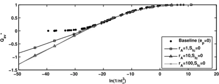
−50 −40 −30 −20 −10 0 10 20 −1.5
−1 −0.5 0 0.5 1
ln(1/ntc 3
)
Qav
*
Baseline (ep=0) rA=1,Sfc=0
rA=10,Sfc=0
rA=100,Sfc=0
Fig. 3a. Expected value of the annual flood peak, for the non-threshold case including evaporation for different values of the
di-mensionless ratio,rA.
where a and b are empirical coefficients that vary only slightly depending upon T (i.e. a=0.0519 andb=−0.174 forT=10 years, compared toa=0.0534 andb=−0.163 for
T=100 years). Allowing for the scatter associated with the finite simulation length – especially in relation to large re-turn periods – these curves approximately overlap, such that variation in a andb withT is relatively small, i.e. Q∗T is approximately constant for a given value ofntc3. We can re-gardQ∗T, which ranges in value from 0 to 1, as an index of the slope of the flood frequency curve relative to the rain-fall frequency curve. A value ofQ∗T approaching 0 corre-sponds to tc→∞, with flood peaks due to subsurface flow being relatively invariant from one year to another, approx-imately equal toQmin. As Q∗T increases, flood peaks due to subsurface flow will be increasingly impacted by scale variability in storm properties (and consequent event-scale variability in the antecedent condition), such that flood magnitude increases significantly with increasing return pe-riod. AsQ∗T approaches 1, attenuation by the catchment be-comes minimal, and the flood frequency curve has the same slope as (and is therefore equivalent to) the rainfall frequency curve. In summary, the slope and magnitude of the baseline flood frequency curve is functional upon the average values of storm intensity, storm duration, and number of storms per year, which together determine the magnitude ofQmaxT , and the characteristic response time for subsurface flow, which determines the degree of attenuation associated with the rain-fall to runoff transformation.
3.3 Impact of evaporation on subsurface flow flood fre-quency
In terms of the rainfall to runoff transformation, evaporation acts essentially as a loss mechanism. If we consider evap-oration during rainfall to be negligible, evapevap-oration during inter-storm periods is capable of reducing the flood peak in-directly via its impact upon reducing antecedent storage prior to a given storm event. In the absence of a field capacity storage threshold, fast-draining soils (i.e. lowtc) will tend to dry towards zero storage by the end of inter-storm periods even without evaporation, such that the impact of evaporation
−50 −40 −30 −20 −10 0 10 20 −1
−0.5 0 0.5 1
ln(1/ntc 3
)
Qav
*
Baseline (ep=0)
rA=1,rB=0
rA=10,rB=20
rA=100,rB=50
Fig. 3b.Expected value of the annual flood peak, for the case with field capacity threshold and evaporation for different combinations
of the dimensionless ratiosrAandrB.
upon the antecedent condition and hence flood frequency will be negligible. In contrast, for slow-draining soils, the impact of evaporation in reducing the antecedent moisture content will be significant, such that the evaporation will have a no-ticeable impact upon flood frequency. Figure 3a presents the expected value of the annual flood peak in the absence of a field capacity threshold for various strengths of evaporation in contrast to the baseline (no evaporation) case. For val-ues of the x-ordinate greater than−20, which typically cor-responds to values oftc<200 h, evaporation has no impact, such that all curves overlap with the baseline curve. Only for
tc>200 h is the soil sufficiently slow-responding that evapo-rative reduction in the antecedent condition causes a reduc-tion in the average annual flood peak. The magnitude of the evaporative impact obtained from the simulations was found to be a function of the ratio of the per-event expected po-tential evaporation volume to the expected rainfall volume,
rA=
ˆ eptˆb
ˆ
itˆr . Where this ratio is significantly greater than 1, the
behaviour ofQ∗avfor x values less than−20 is approximately linear (on semi-log axes) and relatively unchanging. If the ratio is equal to 0, the baseline expression describes its be-haviour. Where 0<rA<1, the behaviour falls between these two “envelope” curves.
3.4 Impact of field capacity on subsurface flow flood fre-quency
−40 −30 −20 −10 0 10 20 −0.5
0 0.5 1
ln(1/ntc3)
Qav
*
Baseline (ep=0) rA=0.6 (Sfc large) rA=0.9 (Sfc large) rA=1.0 (Sfc large)
Fig. 3c. Expected value of the annual flood peak for the case of extremely large field capacity threshold and evaporation.
−40 −30 −20 −10 0 10 20 −0.5
0 0.5 1
ln(1/ntc3)
Q100
*
Baseline (ep=0)
rA=0.6 (Sfc large)
rA=0.9 (Sfc large)
rA=1.0 (Sfc large)
Fig. 3d.Predictions of the 100 year return period flood peak for the case of extremely large field capacity threshold and evaporation for
different values of the dimensionless ratiorA.
again found to depend uponrA, as well asrB= Sf c
ˆ
eptˆb, the
ra-tio of field capacity storage to the event potential evapora-tion volume, which is a measure of the relative magnitude of potential storage deficit below field capacity. The role of evaporation is to reduce the antecedent storage to below the field capacity threshold and its impact upon flood frequency is maximised where these two ratios are large. Figure 3b il-lustrates how the expected value of the annual flood peak for subsurface flow is modified from the baseline behaviour by the introduction of a field capacity storage threshold, in com-bination with evaporation. ForrA≤1, behaviour is essentially the same as the case without the field capacity threshold (i.e. Fig. 3a) unlessrB>>1. AsrBincreases, the impact of evap-oration below field capacity is manifested as a downward translation of the curves relative to the “evaporation without field capacity” case for the same value ofrA.
Figure 3c shows the impact of evaporation for the case of an extremely large field capacity, rB>1×10⁸; for this sce-nario, the ratio S/Sf c in (5), remains approximately equal to 1 throughout the simulation, such that evaporation occurs at potential rates above and below field capacity. Contrast-ing this to Fig. 3b illustrates the potential importance of the piecewise evaporation assumption in (5) upon resulting flood frequency behaviour. In this scenario, flood frequency be-haviour is found to be highly sensitive to the value ofrA; for values significantly lower than 1, the volume of evapo-ration is low relative to the storm volume, and the impact of evaporation is not significant. AsrAincreases towards 1, the evaporative volume is comparable to the storm volume,
1.01 1.1 1.5 2 5 10 20 50 100 500 10−4
10−3 10−2 10−1
100 101 102
Average Recurrence Interval (yrs)
Normalised Discharge, Q/E[i]
No evap. r
A=1 , rB=10
r
A=2 , rB=5
rA=5 , rB=2 Precipitation
Fig. 3e. Impact of evaporation and field capacity threshold upon flood frequency for different combinations of the dimensionless
ra-tiosrAandrB.
such that the runoff response is highly sensitive to stochas-tic variability in storm properties, and hence the antecedent storage condition. The impact of evaporation is less signif-icant in wetter years associated with higher return periods; Fig. 3d shows the 100 year return period flood peak for the same cases as Fig. 3c. For applications specifically interested in extreme flood events only, therefore, accurate accounting of the complex impacts of evaporation upon flood frequency may not be particularly crucial, especially whererA<1.
Figure 3e presents a partial summary of the impact of evaporation upon flood frequency, showing the impact of in-creasing the value ofepalone (which is manifested as a pro-portional increase in the value ofrA and reduction inrB). This figure provides further insights into the summary results presented above in Figs. 3c and d; higher evaporation relative to storm volume (i.e. higherrA)for a moderately large field capacity results in an increased prevalence of flow cessation, with many years generating no flood response. But at larger return periods, the discrepancy between each curve reduces rapidly, until the impact of evaporation is minor for floods with an average recurrence interval of 100 years or more. Of course, the return period at which these curves converge is dependent upon the values ofrAandrB; where these values are larger, convergence could occur at return periods greater than 100 years.
3.5 Impact of saturation
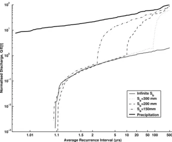
1.01 1.1 1.5 2 5 10 20 50 100 500 10−3
10−2 10−1 100 101 102
Average Recurrence Interval (yrs)
Normalised Discharge, Q/E[i] Infinite S
b
S
b=300 mm
S
b=200 mm
Sb=150mm Precipitation
Fig. 4a.Impact of finite catchment storage capacity, and saturation excess, upon flood frequency.
instantaneous concentration time) than subsurface flow. Figure 4a illustrates the impact of a finite catchment stor-age capacity and resulting saturation excess upon flood fre-quency in contrast to a catchment with infinite storage ca-pacity, and hence no saturation excess. The onset of satu-ration excess results in a significant break in the flood fre-quency curve at a return period associated with the average recurrence interval between years in which saturation excess is triggered. Flood frequency at high return periods even-tually converges towards the rainfall frequency curve (since surface runoff is assumed to be converted instantaneously to a flood response; a finite response time for surface runoff would result in peaks below the rainfall frequency values). The break in curve occurs at lower return periods as the catchment storage capacity reduces. At return periods be-low this break, flood peaks are associated with subsurface flow only, such that this region of the flood frequency curve is not impacted by changes in the value ofSb. Similar breaks or “transitions” in the flood frequency curve have previously been described by Sivapalan et al. (1990), associated with a transition from partial area saturation excess-dominated to infiltration excess-dominated runoff. Where several runoff mechanisms exist, the flood frequency curve may therefore have multiple breaks, each associated with a transition in the dominant runoff-producing mechanism.
Previous work by Struthers et al. (2007) formulated a di-mensionless index of the relative frequency of saturation ex-cess triggering for equivalent rainfall and runoff models as those used here:
α=
ˆ
itc
h
exptˆr tc
−1i
Sb−Sf c
exptˆr tc
−
ˆ
S0−Sf c Sb−Sf c
(13)
−8 −6 −4 −2 0 2 4
0 0.2 0.4 0.6 0.8 1
ln(α)
Qav
**
t
c=100 hrs,ep=0
tc=100 hrs,rA=1,rB=10 t
c=1000 hrs,ep=0
t
c=1000 hrs,rA=1,rB=10
t
c=1000 hrs,rA=10,rB=1
tc=10000 hrs,ep=0 tc=10000 hrs,rA=1,rB=10
α
Fig. 4b. Example relationships between normalised values of the
annual flood peak and the indexαfor different combinations of the
dimensionless ratiosrAandrB.
whereSˆ0is the expected value of antecedent storage, which
in this study is determined a posteriori from analysis of sim-ulation data. This index is a direct re-arrangement of the single-storm criteria for the triggering of saturation excess; for an individual storm with these average properties inci-dent upon a catchment with average anteceinci-dent storage, sat-uration excess will occur only ifα>1. When applied instead to a population of stochastically varying storms, and hence stochastically varying antecedent conditions, α instead re-lates to the per-storm frequency of saturation excess occur-rence, with this relative frequency increasing asαincreases. In the case of a sufficiently large catchment storage capac-ity, even an extreme duration and intensity storm occurring in wet antecedent conditions will be insufficient to generate saturation excess, and flood frequency behaviour is identical to the subsurface flow-only case considered thus far. In the opposite extreme, where the catchment storage capacity is sufficiently small that all storms trigger saturation excess, it is apparent from the summation of (2) and (3) that the an-nual flood peak will correspond to the anan-nual rainfall inten-sity peak. Once more, it is therefore possible to normalise flood frequency behaviour between the subsurface flow only value, which we will denote as Qss, and the rainfall fre-quency value,QmaxT , for a given return periodT:
Q∗∗T = ln(QT)−ln Q
ss T
ln QmaxT −ln QssT (14)
Figure 4b presents example cases of the impact of intermit-tent triggering of saturation excess, which is functional on
α, upon the expected value of the annual flood peak; for a given curve, variation inαis obtained by altering the bucket storage capacity,Sb(noting that this will have a consequent impact in alteringSˆ0). As expected, below some threshold
annual rainfall intensity is still small, and therefore the flood frequency is still significantly belowQmaxT . Only with further increases inαis the occurrence of saturation excess so com-mon that, in most years, its occurrence is concurrent with the annual rainfall intensity peak, and flood frequency is approx-imately equal to the rainfall frequency. Note, however, that the return period at which the break in the flood frequency curve occurs does not necessarily correspond to the average time between saturation excess events; the importance of an-tecedent conditions upon saturation excess triggering means that its occurrence is often clustered in time, i.e. there is a relatively high probability of repeated triggering of satura-tion excess by storms immediately following its initial trig-gering. Due to clustering, in years when saturation excess occurs there is a finite probability that it will occur multiple times. As a consequence, the average time between satura-tion excess triggering (i.e. the average of the full distribusatura-tion) is less than or equal to the return period associated with the break in the flood frequency curve (i.e. the average of the ex-treme value distribution). Nonetheless, increases inαabove the lower threshold value are associated with a reduction in the average time between saturation excess triggering (as im-plied from the results of Struthers et al., 2007), as well as a reduction in the return period associated with the break in the flood frequency curve.
Unlike the description in relation to subsurface flow flood frequency,Qss, the behaviour of flood frequency including saturation excess is still not firmly defined; while behaviour is relatively consistent for a given value oftc, the threshold value ofαassociated with the onset of saturation excess and the degree of curvature changes with changing magnitudes oftcin a manner that is as yet not understood. The indexα is therefore imperfect, but is nonetheless useful in describing the basic process controls upon the frequency of saturation excess occurrence, and its consequent impact upon flood fre-quency.
3.6 Summary
For the simplified rainfall and runoff response assumptions used in this study, Fig. 5 presents a summary of the hetero-geneity in the resulting flood frequency in terms of four re-gions, corresponding to (i) evaporation- and field capacity-controlled flow reduction and cessation, (ii) storm intermit-tency and stochasticity-controlled subsurface flow, (iii) sat-uration excess surface flow limited by satsat-uration triggering frequency, and (iv) rainfall-limited saturation excess surface flow. The transition between regions (i) and (ii) is usually gradual, associated with a reduction in the impact of evapora-tion upon flood peaks in wetter rainfall years. In contrast, the transition between regions (ii) and (iii) is abrupt, due to the significantly quicker response time associated with surface runoff compared to subsurface runoff, which results in order of magnitude changes in the resulting flood peak. Region (iii) refers to the situation where saturation excess is occurring,
1.01 1.1 1.5 2 5 10 20 50 100 500 10−2
10−1 100 101 102 103
Average Recurrence Interval (yrs)
Normalised Discharge (Q/E[i])
Peak Discharge Precipitation
(i)
(ii)
(iii)
(iv)
Fig. 5.Illustration of distinct regions of behaviour and process con-trol within the modelled flood frequency curve.
but does not necessarily occur at the same time as extreme rainfall intensities in a given year, such that flood frequency peaks for a given return period are still significantly below the corresponding rainfall intensity peak. Rainfall frequency provides an upper limit for flood frequency, such that region (iv) contains values of annual flood peak caused by saturation excess which is concurrent with extreme rainfall intensities (i.e. intensities of the same order as the annual rainfall peak in a given year).
Each region essentially has distinct process controls and a very distinct curve shape, such that it would be difficult to fit behaviour with a simple statistical model without introduc-ing significant inaccuracies. Given that statistical approaches are commonly used to obtain estimates of large return period flood magnitudes by extrapolation from short historical flood records, which may not incorporate rare events such as sat-uration excess overland flow, the benefit of a derived flood frequency approach over a statistical approach is readily ap-parent.
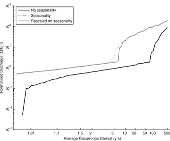
1.01 1.1 1.5 2 5 10 20 50 100 500 10−3
10−2 10−1 100 101 102 103
Average Recurrence Interval (yrs)
Normalised Discharge (Q/E[i])
No seasonality Seasonality Rescaled no seasonality
Fig. 6.The impact of seasonality upon flood frequency. Also illus-trated is the ability to approximately account for simple seasonal-ity implicitly using appropriately scaled average parameter values without seasonality.
3.7 Impact of seasonality
The analysis thus far considered the impact of threshold non-linearities upon flood frequency in response to climate forc-ing with stochastic variability at within-storm and between-storm scales, but without deterministic variability associated with seasonality. It is beyond the scope of a conceptual study such as this to consider the full complexity of seasonal vari-ability in storm and inter-storm properties associated with, for example, seasonal differences in storm type (e.g., synop-tic versus cyclonic rainfall). We simply wish to illustrate the impact that seasonal variability in storm properties, evapora-tion, and hence antecedent conditions, could have upon flood frequency. Seasonality is incorporated in the rainfall genera-tor using a simple sinusoidal variability in average sgenera-torm and interstorm properties, of the form:
ˆ
xt =x+xasin
2π
ωh
(t−t′)
(15) wherexˆt is the average value of the property in question (i.e. storm duration, interstorm period, potential evaporation rate, average storm intensity), for use in (1),x is the sinusoidal mean value, xa is the seasonal amplitude, t is the hour of the year, andt′ is the phase lag in hours. As with the origi-nal (non-seasoorigi-nal) methodology, the actual value of a given realisation of storm duration, interstorm period, and average storm intensity is considered to be stochastically variable (i.e. withxˆt as the mean value of the stochastic distribution at timet ), while potential evaporation is non-variable (i.e. with a value equal toxˆt at timet ). Our examination of seasonality impacts is restricted to the case of out-of-phase seasonality between “wetting” and “drying” climate elements; i.e.
sea-sonality in storm duration and average storm intensity are considered to be perfectly in phase with one another, and of opposing phase to interstorm period and potential evapora-tion seasonality. This “wet season-dry season” simplificaevapora-tion is reasonable for most non-tropical climates.
For flood frequency, which is concerned with annual ex-tremes rather than the complete stochasticity of flood re-sponse, we would expect seasonality to have two types of impact: a direct impact, in terms of longer or more intense storms in a given season, leading to larger runoff response, and an indirect impact associated with seasonality in the an-tecedent condition resulting from seasonality in storm prop-erties. Seasonality in antecedent moisture will be lagged to some degree relative to seasonality in storm properties, such that it probably will not simply be a case of applying the methodology previously described using “wet season” aver-age climate parameters in place of seasonally-averaver-aged cli-mate parameters. Indeed, it was found that a given “wet season-dry season” scenario could be reasonably replicated by a “no seasonality” scenario in which the required param-eter values (i.e.tˆr,tˆb,ˆiandep)were obtained by modifying the sinusoidal average values as appropriate (i.e. increased for wetting climate elements, decreased for drying climate el-ements) by approximately 50% of the seasonal amplitude. In other words, a case in whichxais non-zero for a given prop-erty can be approximately replicated by a case in whichxais assigned a value of zero, andxis appropriately modified. For example, a climate with an 11 hr sinusoidal mean storm dura-tion with 4 hr seasonal variability in this value can be approx-imately replicated by assuming a 13 h average storm duration without seasonal variability; seasonality in average storm in-tensity can be similarly accounted for. Conversely, if poten-tial evaporation varies seasonally with a 0.1 mm/hr sinusoidal average with 0.04 mm/hr seasonal variability, this can be ap-proximately replicated by using a value of 0.08 mm/hr with-out seasonal variability; seasonality in the average interstorm period can likewise be accounted for.
−8 −6 −4 −2 0 2 4 0
0.2 0.4 0.6 0.8 1
ln(α)
Qav
**
ep=0,β=0 r
A=1,rB=10,β=0
e
p=0,β=1
rA=1,rB=10,β=1
α
β
Fig. 7a.Impact of variable soil depth and partial saturation upon the
αrelationship with the normalised expected annual flood peak for
different combinations of the dimensionless ratiosrA andrB and
the parameterβof the Xinanjiang distribution.
reasonably replicate the flood frequency of a seasonally-variable climate.
3.8 Impact of landscape spatial variability
A lumped representation of the catchment was employed in this study so far, which ignores the impact of spatial variabil-ity in the timing and intensvariabil-ity of rainfall, as well as spatial organisation in landscape properties. Issues of spatial scale and spatial variability are considered in detail in other stud-ies (e.g. Bl¨oschl and Sivapalan, 1997; Jothityangkoon and Sivapalan, 2001); this study restricts itself to considering the impact of simple spatial organisation in soil depth, and con-sequent spatial variability in threshold triggering, upon flood frequency. Soil depths are considered to vary with distance away from the stream according to the Xinanjiang distribu-tion (Wood et al., 1992), where the depth of bucketi in a series ofnbuckets is given by:
Sb,i=Smax
"
1−
1−i−0.5
n
1/β#
(16) where Smax is effectively a scaling coefficient for all soil
depths andβ is a shape parameter. Buckets are considered to be connected in series, from deepest to shallowest, with the characteristic response time for subsurface flow in each bucket,tc,i, being equal. The impact of spatial variability in soil depth is assessed by comparing the obtained flood fre-quency against the flood frefre-quency for a lumped catchment with the same average soil depth, i.e.Sb=ESb,i, and with an equivalent catchment-scale characteristic response time for subsurface flow,tc=ntc,i. Note that the multiple bucket case withβ=0 behaves identically to the single-bucket case with equivalent average soil depth and catchment-scale char-acteristic response time for subsurface flow, such that there is no discretisation artefact.
Figure 7a provides an example of the impact of spatial variability in soil depth upon the triggering of saturation ex-cess; the value ofαis calculated for the equivalent single-bucket case, but response behaviour relates to a variable soil depth. As for Fig. 4a, variation in αis obtained by alter-ing the bucket storage capacity,Sb, and the onset of (partial)
1.01 1.1 1.5 2 5 10 20 50 100 500 10−4
10−3 10−2 10−1 100 101
102 103
Average Recurrence Interval (yrs)
Normalised Discharge, Q/E[i]
β = 0
β = 0.1
β = 1
β = 10
Fig. 7b. The impact of variable soil depth and partial saturation upon flood frequency.
saturation is associated with normalised flood peak values greater than 0. The impact of variable soil depth is to create shallower-than-average buckets, which will saturate at lower values ofα compared to the single-bucket case; the larger the value ofβ, the smaller the shallowest bucket depth is, and partial saturation excess onset will occur at progressively lower values ofα. Figure 7b illustrates the impact of partial saturation upon the flood frequency curve. For small values ofβ, which are associated with reductions in the near-stream soil depth, but relatively constant soil depths away from the stream, the incidence of flow cessation is significantly re-duced, and (partial) saturation becomes more common. Asβ
becomes larger, partial saturation occurs in most or all years, such that flood magnitudes at low return periods are signifi-cantly increased. Conversely, extreme flood magnitudes as-sociated with large return periods are reduced by the impact of variable soil depth; in effect, partial saturation increases the efficiency of runoff generation and reduces the overall retention of water in the catchment at any point in time, such that full saturation (i.e. 100% of the catchment) rarely if ever occurs.
4 Conclusions
In the absence of thresholds, runoff is produced by a sin-gle mechanism; in this study, subsurface flow. Deviation of flood frequency from rainfall frequency for this single mech-anism will be functional upon the characteristic response timescale associated with the runoff generation and routing processes (i.e. attenuation) and non-runoff losses which im-pact antecedent conditions and runoff recession (e.g., evapo-ration).
The addition of thresholds introduced a multiplicity of intermittently-active runoff generation pathways; deviation of flood frequency from rainfall frequency will therefore be heterogeneous, with different ranges of return period associ-ated with different regimes of runoff pathway activity. Acti-vation of a given flow pathway is conditional upon thresh-old exceedence, such that the transition from one regime to another will depend upon the frequency of threshold ex-ceedence. For storage-based thresholds, the relative fre-quency of threshold exceedance depends upon the value of the threshold itself, properties of rainfall forcing including deterministic and stochastic variability, and non-runoff losses which impact the antecedent condition. The degree of hetero-geneity in the flood frequency curve will therefore be max-imised where there is a wide discrepancy between the re-sponse timescales associated with each runoff mechanism, and where the per-storm frequency of threshold exceedence is greater than 0 but less than 1.
Temporal variability in storm properties associated with seasonality always has the impact of increasing the magni-tude of the flood frequency response associated with a given runoff process, and is likely to increase the frequency of threshold exceedence, relative to a non-seasonal case with the same average storm properties. Spatial variability in landscape properties and climate properties results in spatial variability in the local frequency of threshold exceedence, with the nature of landscape spatial variability being crucial in determining how this impacts upon catchment flood fre-quency. For decreasing soil depth towards the stream, for example, partial saturation (i.e. threshold exceedance in a temporally-variable proportion of the total catchment area) results in a masking of the impacts of threshold behaviour upon the resulting flood frequency; nonetheless, flood fre-quency behaviour remains heterogeneous.
Acknowledgements. The authors wish to acknowledge funding
support provided through an Australian Research Council (ARC) Discovery Grant awarded to the second author. SESE Reference 053.
Edited by: L. Pfister
References
Atkinson, S. E., Woods, R. A., and Sivapalan, M.: Climate
and landscape controls on water balance model complexity over changing timescales, Water Resour. Res., 38(12), 1314, doi:10.1029/2002WR001487, 2002.
Bl¨oschl, G. and Sivapalan, M.: Process controls on regional flood frequency: coefficient of variation and basin scale, Water Resour. Res., 33(12), 2967–2980, 1997.
Eagleson, P. S.: Dynamics of flood frequency, Water Resour. Res., 8(4), 878–898, 1972.
Gupta, V. K., Castro, S. L., and Over, T. M.: On scaling exponents of spatial peak flows from rainfall and river network geometry, J. Hydrol., 187, 81–104, 1996.
Jothityangkoon, C. and Sivapalan, M.: Temporal scales of rainfall-runoff processes and spatial scaling of flood peaks: Space-time connection through catchment water balance, Adv. Water Re-sour., 24(9–10), 1015–1036, 2001.
Kiem, A. S., Franks, S. W., and Kuczera, G.: Multi-decadal variability of flood risk, Geophys. Res. Lett., 30(2), 1035, doi:10.1029/2002GL015992, 2003.
Kusumastuti, D. I., Struthers, I., Sivapalan, M., and Reynolds, D. A.: Threshold effects in catchment storm response and the occur-rence and magnitude of flood events: implications for flood fre-quency, Hydrol. Earth Syst. Sci. Discuss., 3, 3239–3277, 2006, http://www.hydrol-earth-syst-sci-discuss.net/3/3239/2006/. Manabe, S.: Climate and the ocean circulation, 1, The atmospheric
circulation and the hydrology of the Earth’s surface, Mon. Wea. Rev., 97(11), 739–774, 1969.
Merz, R. and Bl¨oschl, G.: A process typology of regional floods, Water Resour. Res., 39(12), 1340, doi:10.1029/2002WR001952, 2003.
Pattison, A., Ward, J. K. G., McMahon, T. A., and Watson, B. (Eds.): Australian Rainfall and Runoff: Flood Analysis and De-sign, The Institution of Engineers, Australia, p. 160, 1977. Robinson, J. S. and Sivapalan, M.: Temporal scales and
hydrologi-cal regimes: Implications for flood frequency shydrologi-caling, Water Re-sour. Res., 33(12), 2981–2999, 1997.
Sivapalan, M., Wood, E. F., and Beven, K. J.: On hydrological sim-ilarity 3. A dimensionless flood frequency model using and gen-eralised geomorphologic unit hydrograph and partial area runoff generation, Water Resour. Res., 26(1), 43–58, 1990.
Sivapalan, M. and Bl¨oschl, G.: Transformation of point rainfall to areal rainfall: Intensity-duration-frequency curves, J. Hydrol., 204, 150–167, 1998.
Struthers, I., Hinz, C., and Sivapalan, M.: Conceptual examination of climate-soil controls upon rainfall partitioning in an openfrac-tured soil II. Response to a population of storms, Adv. Water Resour., 30(3), 518–527, doi:10.1016/j.advwatres.2006.04.005, 2007.