www.nat-hazards-earth-syst-sci.net/8/991/2008/ © Author(s) 2008. This work is distributed under the Creative Commons Attribution 3.0 License.
and Earth
System Sciences
Risk assessment of atmospheric emissions using machine learning
G. Cervone1, P. Franzese1, Y. Ezber1,2, and Z. Boybeyi1
1College of Science, George Mason University, Fairfax, VA 22039, USA
2Eurasia Institute of Earth Sciences, Istanbul Technical University, Istanbul, 34469, Turkey
Received: 28 November 2007 – Revised: 16 May 2008 – Accepted: 25 July 2008 – Published: 9 September 2008
Abstract.Supervised and unsupervised machine learning al-gorithms are used to perform statistical and logical analysis of several transport and dispersion model runs which sim-ulate emissions from a fixed source under different atmo-spheric conditions.
First, a clustering algorithm is used to automatically group the results of different transport and dispersion simulations according to specific cloud characteristics. Then, a symbolic classification algorithm is employed to find complex non-linear relationships between the meteorological input condi-tions and each cluster of clouds. The patterns discovered are provided in the form of probabilistic measures of contamina-tion, thus suitable for result interpretation and dissemination. The learned patterns can be used for quick assessment of the areas at risk and of the fate of potentially hazardous con-taminants released in the atmosphere.
1 Introduction
In applications related to air quality monitoring, homeland security and hazard response, it is necessary to identify in near real time the areas at risks from potentially harmful at-mospheric pollutants. Using high-resolution mesoscale me-teorological models, it is possible to study the transport and dispersion (T&D) of contaminant particles with a certain ac-curacy, and to determine the levels of mean concentration and dosage at the ground.
A complete transport and dispersion simulation consists of different stages. Large scale meteorological data derived from ground observations, remote sensing and global scale model output are processed by mesoscale atmospheric mod-els to predict local meteorological fields. Such fields, along with locations and characteristics of the pollutant sources,
Correspondence to:G. Cervone ([email protected])
are used by T&D models to estimate concentration fields and other variables of interest. At a given location, the probabil-ity of contamination associated to a source can be estimated running an ensemble of mesoscale meteorological and T&D simulations spanning the climatological input conditions of a certain period, e.g., a few months. Although such statistics represent an immediate assessment of risk associated with a given source, they only identify a general risk over the entire time period, failing to specify the areas at risk under specific meteorological conditions. This type of information may be important for emergency response operations.
The proposed method requires information on the source characteristics and an extensive database of concentration at several sampling points associated with a number of at-mospheric releases occurred under different meteorological conditions. The concentration data can be obtained by re-mote sensing observations, ground-based samplers, or atmo-spheric transport and dispersion simulations.
The databases of concentration and meteorological condi-tions are investigated using data mining. In brief, data min-ing consists in the automated analysis of massive amounts of data and background information to generate new predictions through the use of algorithms from different disciplines, such as machine learning and statistics. Most data mining meth-ods are domain independent, and can be applied to different types of problems with little or small modifications.
gorithms in the atmospheric sciences can be found in Gard-ner and Dorling (1998). Marzban (1995, 1997, 1998) and Hsieh (2003) have used artificial neural networks to improve model forecasts of tornadoes, wind predictions, precipitation and rare events. Montero et al. (2005) have used genetic al-gorithms to improve local parameters for wind models. Arti-ficial neural networks are machine learning classifiers which map a set of input attributes into a boolean or multivalued output attribute class. After being trained with several ex-amples, the network is fed an unknown event, and returns a value indicating to which class the event belongs to. Ar-tificial neural networks are usually suited for large nonlin-ear problems, because they are able to lnonlin-earn very complex boundaries. However, they provide no information on why events have been classified in a particular way (Mitchell, 1997). Genetic algorithms usually evolve a population of candidate solutions by mutating or crossovering attributes in a pseudo-random fashion, performing the optimization ac-cording to a distance measure. Unlike neural networks, the results are in the form of vectors of attribute-value pairs, which can be inspected analytically for correctness. They are simple, domain independent, and have been successfully applied to a broad range of problems (Goldberg, 1985). On the other hand, they are slow and prone to converge to local solutions.
In this study, we will use theK-means algorithm (Mac-Queen, 1967; Hartigan and Wong, 1979; Lloyd, 1982) to group together contaminant clouds which display common features in their ground concentration fields. Specifically, the algorithm divides all simulated clouds into groups accord-ing to attributes such as maximum distance from the source, plume spread, main plume direction, and straightness of the centerline. Then, a classification procedure is implemented where a symbolic divide and conquer machine learning algo-rithm (Mitchell, 1997) is used to discover patterns within the meteorological input parameters. Each pattern is associated with one or more groups of clouds. When a new set of mete-orological conditions is considered, it is expected to display one of the patterns already identified, and can thus be imme-diately associated with the corresponding risk map, without requiring a new dispersion simulation.
The paper is organized as follows. Section 2 includes a de-scription of the statistical properties of the releases that are relevant to this study, and details of the technique used to estimate the statistics. In Sect. 3, we describe the machine learning method and how it is applied in the context of an at-mospheric dispersion problem. Section 4 contains an appli-cation of the methodology to a simple case study, consisting of a one year of weekly releases from a fixed point simulated by a mesoscale meteorological model coupled with a trans-port and dispersion model. A brief analysis of the results is also included, along with a discussion of the symbolic ma-chine learning approach adopted here.
We consider releases with a duration much longer than the atmospheric turbulence time scale. Because of the local and regional large-scale atmospheric motions, the wind direction could change significantly, causing overlapping between dif-ferent areas of the same cloud. Therefore, the statistical characteristics of the contaminant clouds cannot be estimated statically by simple geometric relationships, namely from the one-time probability distribution of particles in space, but need to take into account the time history of the particles. Meaningful properties are defined by cloud statistics condi-tional on the age of the particles. This approach also allows the inclusion of chemistry in case of reactive particles, and can account for depletion phenomena such as dry and wet deposition. In this study we focus on the concentration statis-tics at the ground, and therefore we will consider only surface concentration distributions. A box-counting technique was used to calculate the cloud statistics at equally spaced times. An equal number of bins was used to discretize the age of all particles of each cloud. The fixed number of bins ensures a statistically significant sample of particles in each bin, while still providing a good spatial detail of the cloud. Specifically, the total number of particles was divided into nine sets, ac-cording to their age. For each set, a box was computed to contain all the particles. Because the plume spread is neither stationary nor homogeneous in space, the boxes frequently overlap. The statistics of each box are calculated based only on the particles associated to that box.
2.1 Plume Centerline
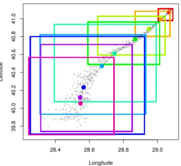
In order to characterize the emissions, the first quantity that needs to be determined is the location of the centerline of the plume which, in general, will not be a straight line. The centerline location of the cloud has been estimated as:
hx, t|τpi =
Z Z
xp(x, t|τp)dx (1)
wherex=(lon, lat) is the two-dimensional vector defining the position of a particle, andp(x, t|τp)is a probability density function representing the probability that a particle be located atx at timet, given that the time elapsed since its release (i.e. its age) isτp.
28.4 28.6 28.8 29.0
39.8
40.0
40.2
40.4
40.6
40.8
41.0
Longitude
Latitude
Fig. 1. Example of center line calculation using the box counting
technique. The particles, shown as gray circles, are grouped into 9 sets according to their age. Each box encompasses the particles of the set, and the matching color solid circle is the center of mass for the box.
2.2 Plume spread
The second quantity used to characterize a plume is its spread, which was also estimated conditional on the age of the particles:
σx2= hx
2, t
|τpi − hx, t|τpi2
=
Z Z
(x− hx, t|τpi)2p(x, t|τp)dx (2)
Equation (2) was estimated at the same center point locations as Eq. (1). The local direction of the plume at each sampling location was assumed parallel to the direction defined by the straight line through the previous and the following center points (see Fig. 2), rather than the exact tangent through the sampling center point. This approximation carries a negligi-ble error, and avoids the additional calculation of the cen-terline at neighboring points necessary to define the exact tangent. The variance at each center point is based on the squared distance of all particles in the associated box to this derived line, according to Eq. (2). This method was chosen over orthogonal statistical regression to preserve information about the local direction of the plume. Orthogonal regression finds the line which minimizes the sum squared distance of the particles. However, a regression does not ensure that the best fit line corresponds to the local direction of the plume. For example, in case of very large variance, the best fit line is likely to be orthogonal to the direction of the plume, rather than parallel to it.
28.75 28.80 28.85 28.90 28.95 29.00 29.05
41.25
41.30
41.35
41.40
41.45
41.50
41.55
Longitude
Latitude
28.95 28.97 28.99 29.01
41.33
41.35
41.37
41.39
Fig. 2.Illustration of the definition of local direction of the plume. The local direction of the plume at a center point is defined as the direction of the straight line through the previous and the following center points.
2.3 Calculation of concentrations and risk assessment The risk associated to an area is represented by the concen-tration at the ground, and is assessed by computing the cu-mulative concentrations at each center points from all cases considered, namely the sum of all concentrations generated by all emissions. This is in fact no longer a concentration calculation, but an estimate of the probability of observing a given concentration at a given point. A probability surface is then constructed by using a Kriging interpolation (Hastie and Tibshirani, 1986) of the computed cumulative concen-trations. Kriging interpolation was found to give realistic results, but different methods might be employed for other problems.
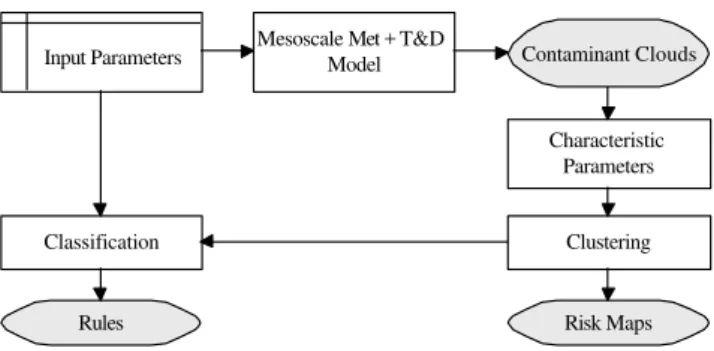
Input Parameters Mesoscale Met + T&DModel
Characteristic Parameters
Clustering Classification
Contaminant Clouds
Rules Risk Maps
Fig. 3. Flowchart illustrating the proposed method. The input
pa-rameters are the set of meteorological observations, remote sensing measurements, and the output of a global scale numerical weather prediction model used to initialize the mesoscale meteorological model, and the parameters for the T&D model. The outputs, shown in gray, are the contaminant clouds, the risk maps and the rules.
homogeneous turbulence. Roberts (1923) obtained the so-lutions to the mean advection-diffusion equation with con-stant eddy diffusivity coefficients in the form of Gaussian functions, and Sutton (1932) obtained a Gaussian function as a solution of the Fickian equation with an “effective eddy” varying with the distance traveled by the cloud. However, the main reason for the popularity of the Gaussian assumption lies in its simplicity and robustness (Hanna, 1982), and in the realization that in practical applications the effect of the shape of the distribution is certainly negligible compared to all other sources of uncertainty such as the turbulent kinetic energy mean dissipation rate, and the expansion rate of the diffusion coefficients, which strongly depends on the fluctu-ating velocity statistics (Pasquill, 1962, p. 192). An ensemble ofN simulated releases is considered. The total number of particles representing each emission is divided intoMsets. The sampling points are chosen corresponding to the center of mass of each box. The normalized cumulative concentra-tionck,mat the center pointmof a given cloudkis computed as the sum of the concentration of the cloudkatmplus the contributions of all the other clouds. The contributions of the other points of the plumekis excluded from the calculations:
ck,m = 1 σk,m +
M
X
j=1 N
X
i=1 i6=k
1 σi,j
exp −
dmj2
2σi,j2
!
(3)
whereσi,jrepresents the standard deviation of the plumeiat the pointj, anddmjis the distance between the pointmand the pointj.
3 Machine learning based method
Machine learning is used to cluster the clouds in a predefined number of groups, and to find patterns of the input parame-ters used for the simulation of each group. Figure 3 shows
put parameters, indicated with the top left rectangle, include the meteorological data used by the mesoscale model as well as the control parameters used by the T&D model. The out-put parameters, indicated with the shaded rounded rectan-gles, are: a) the clusters in which the contaminant clouds have been partitioned, b) their statistical risk maps, and c) the rules which associate each cluster of clouds with pat-terns of meteorological conditions. The operations, indicated with plain rectangles, include running the meteorological and T&D simulations, extracting statistical properties from the contaminant clouds, and the machine learning operations of clustering and classification. The modeling system used for the coupled meteorological and T&D simulations, which will generate the data for the machine learning algorithm, is de-scribed in Sect. 4
3.1 Conceptual representation of the clouds
The machine learning algorithms cluster the clouds based on a number of meaningful attributes. For the current case study, four attributes were considered: main direction, length, straightness, and spread exponent.
Themain directionrepresents the average direction of the centerline. It is defined as the angle formed by the best fit line obtained by a linear regression of the centerline, with respect to a reference direction. The meaningfulness of the direction depends on the shape of the cloud. In cases where the plume is very convoluted, with important changes of direction, the main direction is not representative.
Thelengthis defined as the total streamwise extent of the plume centerline. It is a measure of the distance traveled by a cloud within the total time considered.
The straightness is defined as the distance between the source and the last point of the centerline divided by the length of the centerline. Straightness equal to 1 defines a per-fectly straight plume, whereas smaller values indicate larger departures from a straight line.
The spread of each plume can be approximated by a power law of time. The exponent of this power law will be referred to asspread exponent, and is a simple characterization of the rate of expansion of the plume, as dictated by the local atmo-spheric conditions. The spread exponent was determined by a least square method.
3.2 K-means clustering
centroids, and the best result is chosen according to quan-titative metrics, if available, or subjectively. The algorithm performs the following steps:
1. SelectK clouds which are used as initial cluster cen-troids.
2. Compute the distance between each cloud and the se-lected centroids in terms of the four attributes. Each cloud is associated with the closest centroid, and as-signed to the corresponding cluster.
3. Recalculate all the centroids by selecting the clouds closest to the center of mass of each cluster.
4. Repeat from step 2 until the centroids remain constant.
The total squared distance between each cloud in the clus-ter and the clusclus-ter’s centroid is given by
D(r, γ )= L
X
i=1 K
X
j=1
||ri−γj||2 (4)
whereLis the number of attributes (in our case,L=4),riis a
plume attribute andγjis a cluster centroid. Other metrics can
be used, such as the maximum distance between the elements in the cluster, or the average distance between the clouds and the centroids over all clusters.
3.3 Symbolic machine learningclassification
In the current problem, a classification algorithm is used to find common patterns (or rules) in the National Centers for Environmental Prediction (NCEP) meteorological data, that can be associated to each cluster. The input data consists of a matrix, where the rows are the simulations, and the columns are the NCEP input fields (e.g., sea surface temperature, air temperature, pressure, etc.) averaged over an area of approxi-mately 200×200 km around the source (corresponding to the NCEP grid resolution), plus an attribute indicating the clus-ter associated with each simulation. It is possible to consider meteorological data over larger areas, or different time av-erages of the data. However, the meteorological conditions at the source strongly determine the short and medium range dispersion, and can represent reasonably well the regional meteorology.
Symbolic machine learning methods are a type of super-vised learning, where the answer can be directly inspected and hence accepted or rejected. The algorithm used in this study is an optimized version for atmospheric studies of the AQ20 algorithm, developed by Cervone et al. (2001). AQ-type learning describes a general methodology based on beam search dating back to the mid 1970s, first developed to solve the general covering problem, and later expanded and refined to learn rules for machine learning classification. Several formulations of the AQ methodology exist and have been implemented in a number of programs which iteratively
improved the original formulation to cope with real world re-quirements, such as noisy data, large datasets, and approxi-mations to tradeoff completeness with speed. More details can be found in Shapiro (1987, pp. 185–194) and Mitchell (1997).
As an alternative to AQ-type learning, neural networks and decision tree learning methods were also considered for this study. Neural networks were not chosen because they re-quire long training sets, which were not available, and be-cause they do not produce understandable learned knowledge (neural networks use an internal representation comprised of links and weights which cannot be directly inspected and validated). Decision tree learning, such as C4.5 (Quinlan, 1993), have the ability to learn from limited examples, and to generate knowledge which can be translated into rules. How-ever, decision tree learners use a far simpler representation language which is particularly suited for very large datasets and noisy data, neither of which apply to the current problem. The learning process starts by dividing the clouds in two groups, called positives and negatives. The positive group comprises all the clouds in the cluster for which rules are being learned, while the negative group comprises the re-maining clouds for all other clusters. The algorithm learns from example and counter-example patterns of attributes that characterize the positive group, but that do not hold for the negative group. The patterns are represented by rules. A rule consists of two parts, a consequent and a premise, and is usu-ally indicated by the following notation:
Consequent←−Premise (5)
whereConsequentandPremise are conjunctions of Condi-tions. AConditionis simply a relation between an attribute and a set of values it can take. For example, [X1=1..5] means thatX1can take any value in the interval 1 to 5. Typ-ically the consequent consists of a single condition, whereas the premise consists of a conjunction of several conditions. Equation (6) shows a sample rule relating a cluster of clouds to the input parameters used in the atmospheric model. Such rules aim at identifying the most common combination of in-put parameters within a specific cluster of clouds, that is also different from the combinations corresponding to other clus-ters. The annotationspandnindicate the number of positive and negative clouds covered by this rule, i.e. clouds in the current cluster, and clouds in all the other clusters, respec-tively.
[Cluster=1] ←−[WindDir=N..E] (6)
[WindSpeed>10 m/s]
[Temp>22◦C] :p=11, n=3
of values, internal conjunctions of attributes, and other con-structs. Such a rich representation language means that very complex concepts can be represented using a compact de-scription. However, attributional rules have the disadvantage to be more prone to overfitting with noisy data.
Usually, multiple rules are learned for each cluster, and are called aruleset. A ruleset is a disjunction of rules, meaning that even if only one rule is satisfied, then the consequent is true. Multiple rules can be satisfied at one time because the learned rules could be intersecting each other. Equation (7) shows a sample ruleset:
[Cluster=1] ←−[WindDir=N..E] (7)
[WindSpeed>10 m/s]
[Temp>22◦C] :p=11, n=3
←−[WindDir=E]
[Date = July] :p=5, n=0
←−[Pressure>1010]
[Date = Sep] :p=1, n=0
Of course, each rule has a different statistical value. For example, assuming there were 13 clouds in cluster 1, the first rule in Eq. (7) covers most clouds in the cluster (i.e. 11 clouds), but also 3 clouds in other clusters. The second rule covers less than 50% of the clouds and the third covers only 1, but both without covering any clouds in other clusters. Therefore there is a trade-off between completeness, namely the number of clouds covered out of all the clouds in the cluster, and consistency, namely the coverage of clouds from other clusters. The ideal case is a rule covering all clouds in a given cluster, and no clouds in any other cluster.
AQ-type learning presents many important characteristics for this type of problems. First of all, it generates attribu-tional rules that involve conditions that may include nal disjunctions of attribute values, ranges of values, inter-nal conjunctions of attributes, and other constructs. Such conditions make the representational language very expres-sive, potentially learning rules that better describe the com-plex interactions between the meteorological attributes and the clusters of simulations. Another characteristics of AQ-type learning is that given a set of examples, it can gener-ate multiple rulesests depending on the program parameters. The rulesets may be highly general (which may be desirable to identify general areas of potential risks), or highly specific (which may be more desirable to identify high risk facilities), or have an intermediate degree of generality.
4 Case study: the Istanbul channel
The transport and dispersion simulations were performed us-ing the mesoscale atmospheric Operational Multiscale En-vironment model with Grid Adaptivity (OMEGA) (Boybeyi
atmospheric model with an adaptive grid. The terrain-following grid is based on unstructured triangular prisms in a rotating Cartesian coordinate system. The model uses a finite-volume flux-based numerical advection scheme de-rived from Smolarkiewicz (1984). Turbulence parametriza-tion is accomplished by the 2.5 level closure model of Mellor and Yamada (1974). For the surface layer, Beljaars and Holt-slag (1991) formulations are used. The model contains sur-face layer physics with multiple soil layers and 12 soil types. The land surface module is based on the scheme proposed by Noilhan and Planton (1998). OMEGA can use global datasets for soil type and moisture, land use/land cover, veg-etation index, land/water mask, terrain height, sea surface temperature, and subsurface temperature. The microphysics package is derived from Lin et al. (1983), and falls under the category of bulk-water microphysics in which the pro-duction rates are functions of the total mass density of each water species which are vapor, cloud droplets, ice crystals, rain and snow fields. Radiation parametrization is similar to the formulation of Mahrer and Pielke (1977). The radiative source and/or sink terms in the conservation of energy equa-tion is calculated from the temperature change resulting from longwave and shortwave radiative divergence flux in the ver-tical direction. The method of parametrizing this verver-tical flux takes into account the absorption of shortwave radiation by water vapor and the longwave energy emitted by water vapor and carbon dioxide.
The release point was located at the entrance of the Istan-bul channel, Turkey. The simulation domain is located be-tween 52◦N–12.05◦E and 30◦N–44◦E. OMEGA was set up with 35 vertical layers, and three nested domains. The coarse grid has 60 km horizontal resolution while the inner domain, focused on the Marmara Region, was discretized with 2 km horizontal resolution. Initial and boundary conditions were provided by the NCEP global meteorological datasets with a resolution of 2.5◦ latitude× 2.5◦ longitude and 17 ver-tical levels. This database is generated taking into consid-eration measurements at various worldwide stations and re-trieved from satellites.
The dispersion simulations were generated by the La-grangian particle atmospheric dispersion model (ADM) em-bedded in OMEGA. The ADM simulates the dispersion of pollutants in the atmosphere by a large number of tracer par-ticles moving at each time step. It is composed of an algo-rithm that advects tracers using the OMEGA-resolved wind field plus a diffusion model that simulates the effect of the unresolved subgrid-scale turbulence. The subsequent posi-tions(x, y, z)of each particle representing a discrete element of pollutant mass are computed as:
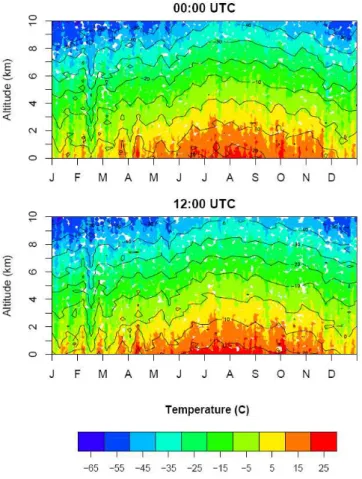
Fig. 4.Vertical temperature readings from meteorological balloons deployed near the simulated source for year 2004. The top graph shows the temperature profile for 00:00 UTC, and the bottom graph for 12:00 UTC.
whereu, v, and w are the OMEGA-predicted mean wind components, and u′, v′, and w′ are the corresponding subgrid-scale turbulent velocity fluctuations in each of the three directions. The subgrid-scale turbulent velocity fluc-tuations are derived from a first-order Markov chain scheme (Boybeyi et al., 2001).
The simulations were performed weekly for year 2004, and include 53 runs. Transport and dispersion were simu-lated for 6 h after the start of each release. The number of simulations and their temporal frequency were determined after an analysis of the local climatic conditions. Figure 4 shows the vertical temperature profile as a function of time for year 2004, at 00:00 UTC (top) and 12:00 UTC (bottom). The data was collected by the Turkish State Meteorological Service using meteorological balloons which measured tem-perature, humidity, wind speed and direction at several verti-cal levels. The balloons were released from the Goztepe sta-tion, located at 40◦58′N–29◦05′E. As Fig. 4 shows, the 53 simulations, performed at regular intervals, sample the range of potential conditions. In other words, taking into account the observed temperature variability, weekly simulations are
Fig. 5. Map of the area with overlay of the 53 simulations
per-formed. The source of the emissions is located at the entrance of the Istanbul channel (Black sea side).
expected to be reasonably representative of the conditions of the region.
4.1 Results
Figure 5 shows the area of the case study and an overlay of the 53 simulations performed. The red solid circles are the particles representing the contaminant. The black lines are the centerlines of each plume, and are computed using the method discussed in Sect. 2.1. Colors indicate the terrain height and sea depth. Higher elevation is shown in bright yellow, lower sea depth in dark blue.
The clouds from all 53 simulations were classified into 6 clusters. Each cluster is then associated with the probability distribution of contamination of the area, i.e. the risk. Risk maps for the 6 clusters were computed using the method de-scribed in Sect. 2.3, based on the analysis of ground con-centrations for all clouds in the cluster. Figure 7 shows the centerlines for each release and the risk probability computed for each cluster. Note that because the characteristics of the source are constant, the difference in spread and length be-tween clouds is only due to different meteorological condi-tions.
S
E
W 5 %
10 %15 % 20 %25 %
30 %35 %
(a) 0 to 100 meters
N
S
E
W 5 %
10 %15 % 20 %25 %
30 %35 %
(b) 100 to 1000 meters
N
S
E
W 5 %
10 %15 % 20 %25 %
30 %35 % 1000m − 3000m
(c) 1000 to 3000 meters
N
S
E
W 5 %
10 %15 % 20 %25 %
30 %35 % 3000m − 10000m
(d) 3000 to 10000 meters
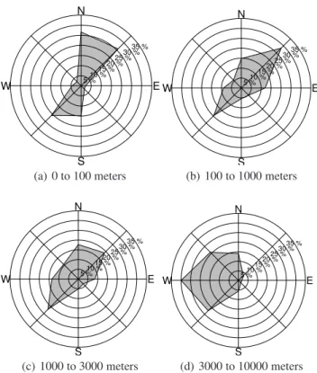
Fig. 6. Dominant wind directions for different vertical intervals
from meteorological balloons deployed near the simulated source at 00:00 UTC and 12:00 UTC for year 2004. (a)0 to 100 m,(b)
100 to 1000 m,(c)1000 to 3000 m and(d)3000 to 10 000 m.
Table 1.Distribution of the simulations across clusters and
proba-bility of the occurrence of each cluster.
Cluster ID Simulation ID Probability
1 11 25 39 40 8%
2 2 7 10 12 14 16 17 18 22 23 24 26 27 28 29 30 31 32 34 35 36 37 38 41 42 43 45 46
50 51 52 58%
3 20 53 4%
4 1 9 4%
5 4 33 48 6%
6 3 5 6 8 13 15 19 21 44 47 49 20%
(Fig. 6d). Consistently with the wind direction statistics, the plumes are expected to have a prevailing NE or SW direction. However, the direction of the plume is not the only funda-mental parameter in the characterization of the cloud. Con-ditions such as atmospheric stability, humidity, temperature gradients, and others, play an important role in determining the dispersion of the contaminants.
Table 1 shows the member simulations for each cluster, and the probability that the risk map associated to each
clus-40.6
41.0
41.4 1 2
40.6
41.0
41.4 3 4
40.6
41.0
41.4
28.6 29.0 29.4 5
28.6 29.0 29.4 6
Risk
0 0.1 0.21 0.34 0.48 0.62 0.76 0.9 1
Fig. 7.The six clusters in which the 53 simulated clouds have been
grouped, and contour plots of the risk probabilities.
ter is valid if a release occurs at the source. The simula-tions areidentified with a sequential number ranging from 1 to 53, which also indicates the time of the year for the re-lease (1 corresponds to 1 January, 2 to the 8th and so on). The number of clouds in each cluster varies from 2 to 31. In the Istanbul example, the area of highest risk is identified by cluster 2, which includes mainly clouds expanding in the south-westerly direction downwind of the source. This result is consistent with the wind analysis (Fig. 6), where north-east and south west were identified as the most probable wind directions for the region throughout the year. Also, all the plumes in cluster 2 are typically straight, and have a limited spread around the centerline.
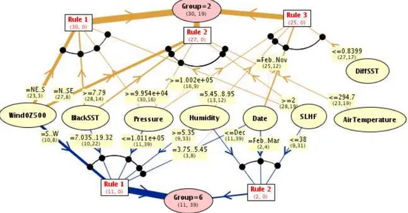
Fig. 8.Graphical visualization of a subset of the rules learned for clusters 2 and 6. The tickness of the links indicate the weight of the rules.
is likely to be affected, given the initial weather parameters, is given by the rules discovered by the machine learning pro-gram, described in Sect. 3.3. More precisely, the rules deter-mine a priori which cluster will best describe the dispersion of a potential release according to the weather conditions, and the risk map associated with it.
Figure 8 is a graphical illustration of the rules discovered from clusters 2 and 6, those with highest probability of oc-currence. Each cluster is associated only with unique pat-terns of input parameters. The thickness of the links indicate the weight of a particular parameter-value combination in the
definition of the cluster. To perform a risk estimate, the given meteorological conditions should be compared with the terns in the graph. The best match between the learned pat-terns and the given conditions identifies the cluster of simu-lations that are most likely to approximate the contaminant dispersion. The degree of match between the learned rules for each cluster and the meteorological observations can be a rough estimate of the uncertainty in the answer (the higher the degree of match, the more similar the current conditions are to those that generated the simulations in the cluster).
The rules are learned through an inductive inference pro-cess, and they might identify as important parameters condi-tions which are only responsible for secondary effects. It is therefore necessary to inspect and validate the rules, in order to verify that the constraints identified for each cluster have a coherent physical explanation. The ability of learning knowl-edge in a human intelligible format is the main strength of this approach as compared to more traditional methods. We have found that a larger number of simulations is necessary to properly sample the search space of the initial parameters using the machine learning method presented. In particular, clusters that include only about 5 or fewer simulations are
poor representative of an area. However, because the simula-tions uniformly sample the atmospheric condisimula-tions through-out a year, such underepresented areas are also the least likely to occur. Future work will include performing the proposaed analysis in a larger number of simulations, and studying the effect of inter-annual effects through the use of simulations that span more than one year.
The current study is to be intended as a proof of concept for a new methodology to use mesoscale atmospheric and transport and dispersion models, in combination with ma-chine learning algorithms, to provide quick assessments of areas of potential risk. An example of a simple application to the Istanbul region in Turkey was developed, where 53 weekly simulations of a 6-h point source release were per-formed using the mesoscale meteorological model OMEGA driven by real climatological data for the year 2004. The pa-per focuses on the methodology rather than on the applica-tion: in order to increase the statistical meaningfulness of the results, a larger number of simulations is necessary for thor-ough sample of the space of the initial parameters. The pro-posed methodology can fully cope with a much larger num-ber of simulations due to the use of scalable machine learning algorithms.
Acknowledgements. We acknowledge L. Panait for his comments on an earlier version of this manuscript. We also wish to thank the anonymous reviewer for his comments and suggestions. Ezber’s research has been supported by the Scientific and Technological Research Council of Turkey (TUBITAK).
Edited by: A. Mugnai
Arya, P. S.: Air pollution meteorology and dispersion, Oxford Uni-versity Press, 1999.
Beljaars, A. C. M. and Holtslag, A. A. M.: Flux parameterization over land surfaces for atmospheric models, J. Appl. Meteor., 30, 327–341, 1991.
Bishop, C. M.: Pattern Recognition and Machine Learning, Infor-mation Science and Statistics, Springer, New York, 2006. Boybeyi, Z., Ahmad, N. N., Bacon, D. P., Dunn, T. J., Hall, M. S.,
Lee, P. C. S., Sarma, R. A., and Wait, T. R.: Evaluation of the Operational Multi-scale Environment model with Grid Adaptiv-ity against the European Tracer Experiment, J. Appl. Meteor., 40, 1541–1558, 2001.
Cervone, G., Panait, L., and Michalski, R.: The development of the AQ20 learning system and initial experiments, in: Tenth In-ternational Symposium on Intelligent Information Systems, Za-kopane, Poland, 2001.
Gardner, M. W. and Dorling, S. R.:Artificial neural networks (the multilayer perceptron) – a review of applications in the atmo-spheric sciences – application for wind retrieval from spaceborne scatterometer data, Atmos. Environ., 32, 2627–2636, 1998. Goldberg, D. E.: Genetic algorithms and rule learning in dynamic
system control, in Proc. of the International Conference on Ge-netic Algorithms and Their Applications, 8–15, Pittsburgh, PA, 1985.
Hanna, S. R.: A review of atmospheric diffusion models for regu-latory applications, Tech. Rep. 177, World Meteorological Orga-nization, Geneva, 1982.
Hartigan, J. A. and Wong, M.: A K-means clustering algorithm, Appl. Stat., 28, 100–108, 1979.
Hastie, T. and Tibshirani, R.: Generalized additive models, Stat. Sci., 1, 297–310, 1986.
Langley, P.: Elements of Machine Learning, Morgan Kaufmann Publishers, Inc., San Francisco, California, 1996.
Lin, Y.-L., Farley, R. D., and Orville, H. D.: Bulk parameterization of the snow field in a cloud model, J. Clim. Appl. Meteorol., 22, 1065–1092, 1983.
Lloyd, S. P.: Least squares quantization in pcm, IEEE Transactions on Information Theory, 28, 128–137, 1982.
MacQueen, J. B.: Some methods for classification and analysis of multivariate observations, in: Proceedings of 5-th Berkeley Sym-posium on Mathematical Statistics and Probability, vol. 1, 281– 297, University of California Press, 1967.
and land breezes in a two-dimensional numerical model, Mon. Weather Rev., 105, 1151–1162, 1977.
Marzban, C.: A neural network for tornado prediction based on doppler radar-derived attributes, J. Appl. Meteorol., 35, 617–626, 1995.
Marzban, C.: A neural network for damaging wind prediction, Weather Forecast., 16, 600–610, 1997.
Marzban, C.: Scalar measures of performance in rare-event situa-tions, Weather Forecast., 13, 753–763, 1998.
Mellor, G. L. and Yamada, T.: A hierarchy of turbulence closure models for planetary boundary layers, J. Atmos. Sci., 31, 1781– 1806, 1974.
Mitchell, T.: Machine Learning, McGraw-Hill Education (ISE Edi-tions), 1997.
Montero, G., Rodriguez, E., Montenegro, R., Escobar, J. M., and Gonzalez-Yuste, J. M.: Genetic algorithms for an improved pa-rameter estimation with local refinement of tetrahedral meshes in a wind model, Adv. Eng. Softw., 36, 3–10, 2005.
Noilhan, J. and Planton, S.: A simple parameterization of land sur-face processes for meteorological models, Mon. Weather Rev., 117, 536–549, 1998.
Pasquill, F.: Atmospheric Diffusion, D. Van Nostrand Company LTD, 1962.
Quinlan, R. J.: C4.5: Programs for Machine Learning, Mor-gan Kaufmann Series in Machine Learning, MorMor-gan Kaufmann, 1993.
Roberts, O.: The theoretical scattering of smoke in a turbulent at-mosphere, Proc. Roy. Soc. Lond. Ser.-A, 104, 640–654, 1923. Shapiro, S. C. (Ed.): Encyclopedia of Artificial Intelligence, John
Wiley and Sons, 1987.
Smolarkiewicz, P. K.: A fully multidimensional positive definite ad-vection transport algorithm with small implicit diffusion, J. Com-put. Phys., 54, 325–362, 1984.
Sutton, O. G.: A theory of eddy diffusion in the atmosphere, Proc. Roy. Soc. Lond. Ser.-A, 135, 143–165, 1932.
Taylor, G. I.: Diffusion by continuous movements, Proc. Lond. Math. Soc., 20, 196–211, 1921.