www.atmos-chem-phys.net/7/3447/2007/ © Author(s) 2007. This work is licensed under a Creative Commons License.
Chemistry
and Physics
A semi-analytical method for calculating rates of new sulfate aerosol
formation from the gas phase
J. Kazil1,2and E. R. Lovejoy1
1NOAA Earth System Research Laboratory, Boulder, CO, USA 2NRC Research Associateship Programs, Washington, D.C., USA
Received: 8 January 2007 – Published in Atmos. Chem. Phys. Discuss.: 15 February 2007 Revised: 30 May 2007 – Accepted: 15 June 2007 – Published: 2 July 2007
Abstract. The formation of new aerosol from the gas phase is commonly represented in atmospheric modeling with pa-rameterizations of the steady state nucleation rate. Present parameterizations are based on classical nucleation theory or on nucleation rates calculated with a numerical aerosol model. These parameterizations reproduce aerosol nucle-ation rates calculated with a numerical aerosol model only imprecisely. Additional errors can arise when the nucleation rate is used as a surrogate for the production rate of particles of a given size. We discuss these errors and present a method which allows a more precise calculation of steady state sul-fate aerosol formation rates. The method is based on the semi-analytical solution of an aerosol system in steady state and on parameterized rate coefficients for H2SO4uptake and
loss by sulfate aerosol particles, calculated from laboratory and theoretical thermodynamic data.
1 Introduction
Aerosol particles play an important role in the Earth’s atmo-sphere and in the climate system: Aerosols scatter and absorb solar radiation (e.g. Haywood and Boucher, 2000), facili-tate heterogeneous and multiphase chemistry (Ravishankara, 1997), and change cloud characteristics in many ways (e.g. Lohmann and Feichter, 2005). Aerosol particles can either be directly emitted from surface sources (primary aerosol) or form from the gas phase (secondary aerosol). The pro-cesses and compounds involved in secondary aerosol forma-tion and growth, as well as their relative importance, and the spatial and temporal distribution thereof are the subject of ongoing research. The chemical species of interest in-clude inorganic acids, ammonia, and organic molecules (see, e.g. Heintzenberg, 1989; Heintzenberg et al., 2000; Jacobson
Correspondence to:J. Kazil ([email protected])
et al., 2000; Kulmala et al., 2004a, and references therein). Among these, sulfuric acid stands out due to its very low vapor pressure, its numerous sources, and its ubiquity. In clean areas, such as over oceans, sulfuric acid appears as the driving force of secondary aerosol formation (Clarke, 1992; Brock et al., 1995), while over continents and in particular in the continental boundary layer, recently formed aerosol particles contain in addition to sulfate substantial amounts of ammonia (Smith et al., 2005) or organic matter (Allan et al., 2006; Cavalli et al., 2006), which may be involved in their formation process (Coffman and Hegg, 1995; Kulmala et al., 2004b). Secondary aerosol formation can significantly in-crease concentrations of aerosol particles and cloud conden-sation nuclei, and therefore requires dependable representa-tions in atmospheric models (Kulmala et al., 2004a).
2 Representing secondary aerosol formation in atmo-spheric models
Detailed representations of secondary aerosol formation, with a molecular size resolution of the involved processes, are numerically expensive and presently used in box (Lehti-nen and Kulmala, 2003; Lovejoy et al., 2004) or parcel mod-els (Kazil et al., 2007). In medium- and large scale atmo-spheric models, numerically less costly parameterizations of the steady state aerosol nucleation rate are used (e.g. Lauer et al., 2005; Ma and von Salzen, 2006). Aerosol nucleation is the process by which supercritical molecular clusters, par-ticles larger than the critical cluster, form from the gas phase. The critical cluster is the smallest particle whose growth due to uptake of gas phase molecules is uninhibited by a thermo-dynamic barrier.
the determination of the surface tension of small molecular clusters of a given composition, and on the vapor pressures of the involved molecules above the corresponding bulk solu-tion. Modgil et al. (2005) parameterized nucleation rates that were calculated with a numerical aerosol model that resolves the initial steps of cluster formation molecule by molecule.
These parameterizations reproduce aerosol formation rates calculated with numerical aerosol models only imprecisely, for different reasons: On the one hand, the concepts of sur-face tension and bulk solution break down in the context of small molecular clusters. On the other hand, nucleation rates are highly non-linear and vary by many orders of mag-nitude over the atmospherically relevant ranges of ambient conditions. A precise parameterization of the nucleation rate may therefore require a large set of basis functions, with a corresponding number of coefficients, that need to be deter-mined from a sufficiently large nucleation rates table. How-ever, generating a large nucleation rates table with a detailed aerosol model may be numerically prohibitive.
Independently of the intrinsic errors of nucleation rate pa-rameterizations, errors can arise when the nucleation rate is used as a surrogate for the production rate of particles of a given size. We have therefore chosen a different approach for calculating secondary aerosol formation rates. The method is based on the semi-analytical solution of an aerosol sys-tem in steady state, and on parameterized rate coefficients for the uptake and loss of gas phase molecules by aerosol parti-cles. The thermodynamic parameters (entropy and enthalpy change) for the uptake and loss of gas phase molecules by small molecular clusters, which are needed for the calcula-tion of dependable particle formacalcula-tion rates, have been deter-mined in the laboratory only for few atmospherically rele-vant systems: Curtius et al. (2001) and Froyd and Lovejoy (2003a,b) measured the thermodynamic parameters for the formation of charged sulfuric acid and water clusters, while Hanson and Lovejoy (2006) measured the thermodynamic parameters for their neutral counterparts. We therefore fo-cus in the following on the formation of sulfate aerosol from nucleation of neutral and negative sulfuric acid/water parti-cles. The nucleation of positive sulfuric acid/water particles is thought to be less important for aerosol formation at least at temperatures of the lower troposphere (Froyd and Lovejoy, 2003a), and is not considered here.
3 Neutral and negative sulfate aerosol formation
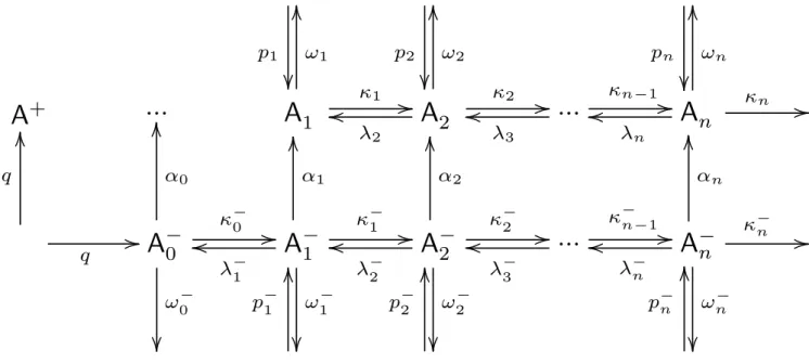
The scheme of neutral and negative H2SO4/H2O aerosol
for-mation from the gas phase is shown in Fig. 1: The ionization rateq is the rate at which the anions A−0 and the cations A+ are produced. Here we assume that A−0=NO−3(HNO3). The
neutral and negative clusters Ai and A−i are defined as Ai =(H2SO4)i(H2O)x(i)
A−i =HSO−4(H2SO4)i−1(H2O)y(i)
, i=1, ..., n. (1)
x(i)andy(i)are the average H2O contents of the clusters
in equilibrium with respect to H2O uptake and loss. A1 is,
as a matter of course, gas phase sulfuric acid, which we will denote in the following simply with H2SO4. The clusters
grow and evaporate with the first order rate coefficients κi =kai· [H2SO4] , λi =kdi ,
κi−=ka−
i· [H2SO4] , λ − i =k
− di .
(2)
kaiandkdi are the H2SO4uptake and evaporation rate coef-ficients of the Ai,ka−i andk
−
di the H2SO4uptake and evap-oration rate coefficients of the A−i , averaged over the equi-librium H2O distribution of the clusters. Theωi andω−i in Fig. 1 are the pseudo first order rate coefficients for loss of the Ai and A−i by coagulation among each other and onto preexisting aerosol. Thepi andpi−are production rates of the Aiand A−i by coagulation of smaller clusters. Theαiare pseudo first order rate coefficients for the recombination of the A−i with the cations A+. The rate coefficients and their calculation are explained in more detail in Sect. 4.
We denote the net steady state formation rate of the Ai and A−i with i>n from the Ai and A−i with i≤n with
J(n, p, q, r, s, t,[H2SO4]). J is a function of pressurep,
ionization rateq, relative humidityr, H2SO4condensational
sinks, temperaturet, and of the sulfuric acid gas phase con-centration [H2SO4]. The pressure dependence ofJ is weak
if the clusters Aiand A−i withi≤nare much smaller than the mean free path of gas phase molecules (typically>100 nm in atmospheric conditions), when their H2SO4uptake and loss
as well as their coagulation take place in the free molecular regime.J can be broken down into three contributions,
J(n, p, q, r, s, t,[H2SO4])=Jcond+Jevap+Jcoag , (3)
where
Jcond=kan[H2SO4][An] +k −
an[H2SO4][A−n] (4) represents for the formation of clusters by condensation of sulfuric acid,
Jevap= −kdn+1[An+1] −k − dn+1[A
−
n+1] (5)
the loss of clusters by evaporation of sulfuric acid, and Jcoag=
n X
i=2 n X
j=max(i,n+1−i)
kci,j[Ai][Aj]
+ n X
i=2 n X
j=n+1−i
kci,j− [Ai][A−j]
(6)
the formation of clusters due to coagulation. The calculation of the coagulation rate coefficientskci,j andk
−
ci,j is explained in Sect. 4.
The smallest neutral cluster whose sulfuric acid contentc satisfies
kac· [H2SO4] ≥kdc
∧ kai · [H2SO4]> kdi ∀i > c
p
1p
2p
nA
+
...
A1
ω
1O
O
κ
1/
/
A2
ω
2O
O
κ
2/
/
λ
2o
o
...
λ
3o
o
κ
n−1/
/
A
n
ω
nO
O
κ
n/
/
λ
no
o
q
/
/
q
O
O
A
−
0
α
0O
O
κ
− 0/
/
ω
− 0A
−
1
α
1O
O
κ
− 1/
/
λ
− 1o
o
ω
− 1A
−
2
α
2O
O
κ
− 2/
/
λ
− 2o
o
ω
− 2...
κ
−n−1
/
/
λ
−3
o
o
A
−
n
α
nO
O
κ
− n/
/
λ
− no
o
ω
− np
− 1O
O
p
− 2O
O
p
− nO
O
Fig. 1.Reaction scheme of a coupled neutral and negative aerosol system.
is the neutral critical cluster. Forn≫c, the particles An+1
and A−n+1evaporate only very slowly, andJevap≈0.
Atmospheric models which account for H2SO4/H2O
par-ticles containing more thannH2SO4 molecules need to be
supplied only with the formation rate
J (n, p, q, r, s, t,[H2SO4])=Jcond+Jcoag (8)
of these particles, since they can either neglectJevapifn≫c,
or otherwise calculate it from the concentrations of the parti-cles they account for. We therefore focus in the following on the particle formation rateJ (n, p, q, r, s, t,[H2SO4]), which
we will refer to as nucleation rate forn=c.
4 Rate coefficients
The rate coefficients for sulfuric acid uptake by the neu-tral and negative H2SO4/H2O aerosol particles are calculated
with the Fuchs formula for Brownian coagulation (Fuchs, 1964). The effect of particle charge is accounted for as de-scribed by Lovejoy et al. (2004). The rate coefficients for sulfuric acid evaporation from the aerosol particles are cal-culated from the uptake rate coefficients and from the ther-modynamic parameters for H2SO4uptake/loss by the
parti-cles, described in Sect. 5. The resulting H2SO4uptake and
loss rate coefficients are averaged over the equilibrium prob-ability distributions of the particle H2O content, giving the
rate coefficientskai,kdi,k−ai, andk −
di. The equilibrium prob-ability distributions of the particle H2O content and the
cor-responding averages are calculated from the thermodynamic parameters for H2O uptake/loss by the particles, described in
Sect. 5.
The rate coefficients kci,j for coagulation of the neutral particles among each other, the rate coefficientsk−ci,j for the coagulation of neutral and negative particles, and the rate co-efficients kpre,i andkpre−,i for their coagulation with preex-isting aerosol are calculated with the Fuchs formula. The masses and diameters of the particles used in the calculation are determined from their H2SO4and average H2O contents.
The effect of the particle charge is accounted for as described by Lovejoy et al. (2004). Charging of the preexisting aerosol particles is neglected.
The pseudo first order rate coefficientsωi andω−i (Fig. 1) for loss of the particles by coagulation with each other and with preexisting aerosol are calculated with
ωi = n X
j=2
(1+δi,j)kci,j[Aj]
+ n X
j=0
kci,j− [A−j] +kpre,i kpre,1
s , i=1, ..., n ,
(9)
and
ω−i = n X
j=2
kc− j,i[Aj] +
k−pre,i kpre,1
s , i=0, ..., n , (10)
with the preexisting aerosol H2SO4 condensational sink s.
The summation over the neutral cluster concentrations[Aj] starts withj=2, because coagulation with A1 is equivalent
to uptake of gas phase H2SO4, which is accounted for by the
The production ratespiof neutral clusters due to coagula-tion read
pi =0 , i=1, ...,3 , pi =
i−2 X
j=2
1+δj,i−j
2 kcj,i−j[Aj][Ai−j] , i=4, ..., n .
(11)
p1equals zero because A1is gas phase H2SO4. Thepi=2,3
equal zero, and the summation giving thepi=4,...,nstarts with 2 and ends withi−2 because coagulation with A1is
equiv-alent to uptake of gas phase H2SO4, which is accounted for
by the H2SO4uptake rate coefficients.
The production ratespi−of negative clusters due to coag-ulation read
p1−=0 , pi−=
i−2 X
j=0
kci−−j,j[Ai−j][A−j] , i=2, ..., n .
(12)
p−1 equals zero and the summation giving thepi−=2,...,nends withi−2 because coagulation with A1is equivalent to uptake
of gas phase H2SO4, which is accounted for by the H2SO4
uptake rate coefficients.
The pseudo first order rate coefficients αi=kri[A+] de-scribe the recombination of the A−i with cations A+, where thekri are the rate coefficients for recombination of the an-ions with the cation population. A mass and size independent recombination rate coefficient kri
.
=kr=1.6×10⁻⁶cm3s−1 (Bates, 1982) is assumed for all anions/cations in this work.
In atmospheric conditions, the mean free path of gas phase molecules is typically>100 nm. H2SO4uptake and loss as
well as the coagulation of particles much smaller than this size take place in the free molecular regime, where the cor-responding rate coefficients are essentially independent of pressure. All rate coefficients were therefore calculated at 1013.25 hPa.
5 Thermodynamic parameters for H2SO4and H2O
up-take and loss
The thermodynamic parameters (entropy and enthalpy change) for uptake and loss of H2SO4 and H2O by the
small negative clusters are based on the laboratory measure-ments of Curtius et al. (2001) and of Froyd and Lovejoy (2003b). The thermodynamic parameters for the formation of (H2SO4)2(H2O)x(2)and of (H2SO4)3(H2O)x(3)due to up-take of sulfuric acid from the gas phase are calculated explic-itly from fits to the laboratory measurements by Hanson and Lovejoy (2006). These fits read, with RH over water in %,
dS(kcal mol−1K−1)= −0.04
dH (kcal mol−1)= −18.32−4.55×10⁻³·RH (13)
for the dimer formation and dS(kcal mol−1K−1)= −0.045
dH (kcal mol−1)= −21.41−2.63×10⁻²·RH (14) for the trimer formation.
The thermodynamic parameters for large aerosol particles are based on the the liquid drop model and on H2SO4 and
H2O vapor pressures over bulk solutions, calculated with a
computer code (S. L. Clegg, personal communication, 2007) that uses data from Giauque et al. (1960) and Clegg et al. (1994). It is assumed that charging of large aerosol has a neg-ligible effect on the uptake and loss of gas phase molecules. The thermodynamic parameters for intermediate size parti-cles are a smooth interpolation of the thermodynamic param-eters for the small and large particles. For the negative par-ticles, the interpolation scheme by Froyd (2002) is used. In the case of the neutral particles, exponential correction terms as introduced by Lovejoy et al. (2004) are added to the liq-uid drop model Gibbs free energies. The correction terms used here are adjusted to match the dimer and trimer data in Eqs. (13) and (14): The term 3 e−(m+n)/5kcal/mol is added
to the liquid drop Gibbs free energies for the addition of a sulfuric acid molecule to a (H2SO4)m−1(H2O)n cluster and for the addition of a water molecule to a (H2SO4)m(H2O)n−1
cluster. The water vapor saturation pressure formulation by Goff (1957) was used in all calculations to transform relative humidity over water to water vapor concentration and vice versa.
6 Parameterization
Calculating H2SO4 uptake and loss rate coefficients as
de-scribed in Sect. 4 is numerically expensive due to the averag-ing of the rate coefficients over the cluster water content. Us-ing parameterized rate coefficients and average cluster water contents can reduce the computational burden. We param-eterize the rate coefficientskai, kdi, k
− ai andk
−
di for H2SO4 uptake and loss by the neutral and negative clusters and the average cluster H2O contentsx(i)andy(i)as functions of
temperaturetand relative humidityrwith a series of Cheby-shev polynomials of the first kindTu(t )andTv(r)up to de-greesu′andv′, respectively:
k(t, r)≈ ˜ku′,v′(t, r)=
u′
X
u=0 v′
X
v=0
αu,vTu t (t )Tv r(r) (15)
withtandrdefined as
t (t )=2t−(t0+t1) t1−t0
,
r(r)=2r−(r0+r1) r1−r0
,
on the temperature and relative humidity intervals t ∈ [t0, t1], t0=190 K, t1=300 K,
r∈ [r0, r1], r0=0.5 %, r1=104 %.
(17)
We determine the coefficientsαu,vforu, v≤20 using an or-thogonality property of the Chebyshev polynomials:
αu,v=
4 π2(1+δ
u,0)(1+δv,0) Z 1
−1
dt Z 1
−1
dr k(t , r)p Tu(t ) Tv(r) 1−(t )2p
1−(r)2 .
(18)
We then measure the error of the approximation (15) with
Eu′,v′ =max
˜
ku′,v′(t, r)−k(t, r)
k(t, r)
(19)
and determine the cutoff ordersu′ ≤20 andv′ ≤20 which minimizeEu′,v′.
7 Semi-analytical solution for aerosol schemes in steady state
7.1 Neutral aerosol
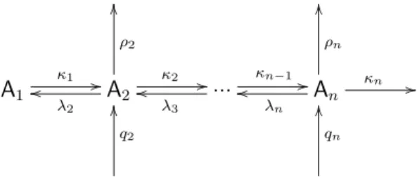
Here we give a semi-analytical solution for the steady state concentrations of the particles Ai=2,...,nin the aerosol scheme in Fig. 2, at a given concentration of the gas phase molecule A1. The particles are produced by sources at the
ratesqi and lost in sinks with the pseudo first order rate co-efficientsρi. They grow by condensation of the gas phase molecules A1with the pseudo first order rate coefficientsκi and decay by evaporation of those molecules with the pseudo first order rate coefficientsλi. Let us start by assuming that the aerosol particles do not interact with each other (no coag-ulation). With the total pseudo first order rate coefficient for loss of the Ai
σi =. κi+λi +ρi , i=2, ..., n (20) the system of differential equations for the concentrations [Ai]reads
d[Ai]
dt =qi−σi[Ai] +κi−1[Ai−1] +λi+1[Ai+1] , i=2, ..., n−1 ,
d[An]
dt =qn−σn[An] +κn−1[An−1] .
(21)
The[Ai]in steady state (d[Ai]/dt=0) can be calculated from this system of equations with
[Ai] =Ri−1[Ai−1] +Si−1 , i=2, ..., n . (22)
A1
κ1 //A2
ρ2
O
O
κ2
/
/
λ2
o
o
...
κn−1
/
/
λ3
o
o
A
nρn
O
O
κn
/
/
λn
o
o
q2
O
O
qn
O
O
Fig. 2.Reaction scheme of a neutral aerosol system.
The coefficientsRiandSiread Rn−1=
κn−1
σn ,
Ri =
κi
σi+1−λi+2Ri+1
, i=n−2, ...,1 ,
Sn−1=
qn
σn ,
Si =
qi+1+λi+2Si+1
σi+1−λi+2Ri+1
, i=n−2, ...,1 . (23)
Loss of the particles by self-coagulation can be accounted for by substituting theσi according to
σi →σi+ n X
j=2
(1+δi,j)kci,j[Aj] , i=2, ..., n . (24)
Production of the particles due to self-coagulation can be ac-counted for by substituting theqiaccording to
qi →qi+ i−2 X
j=2
1+δj,i−j
2 kcj,i−j[Aj][Ai−j] , i=4, ..., n .
(25)
kci,j is the rate coefficient for the coagulation of two parti-cles Ai and Aj, which upon coagulation produce a particle Ai+j. The[Ai]in steady state can then be obtained by iter-ating the solution (22) and (23), starting e.g. with[Ai]=0 for i=2, ..., nand updating the cluster concentrations after each iteration. The[Ai]after the first iteration will be identical with the[Ai]without coagulation.
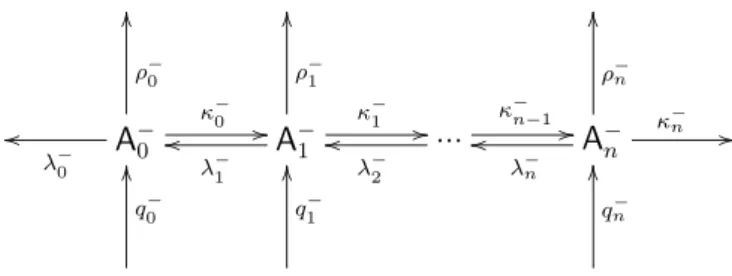
7.2 Negative aerosol
A
− 0 ρ− 0 O O κ− 0 / / λ− 0 oo
A
−1 ρ− 1 O O κ− 1 / / λ− 1 o o
...
κ−n−1
/
/
λ−
2
o
o
A
−nρ− n O O κ− n / / λ− n o o q− 0 O O q− 1 O O q− n O O
Fig. 3.Reaction scheme of a negative aerosol system.
coagulate. With the total pseudo first order rate coefficient for loss of the A−i
σi−=. κi−+λ−i +ρi− , i=0, ..., n (26) the system of differential equations for the concentrations [A−i ]reads
d[A−0] dt =q
− 0 −σ
− 0[A
− 0] +λ
− 1[A
− 1] ,
d[A−i ] dt =q
− i −σ
− i [A
− i ] +κ
− i−1[A
− i−1]λ
− i+1[A
− i+1] ,
i=1, ..., n−1 , d[A−n]
dt =q
−
n −σn−[A−n] +κn−−1[A − n−1] .
(27)
The [A−i ] in steady state (d[A−i ]/dt=0) can be calculated from this system of equations with
[A−0] = q − 0 +λ
− 1S
− 0
σ0−−λ−1R0− ,
[A−i ] =Ri−−1[Ai−−1] +Si−−1 , i=1, ..., n .
(28)
The coefficientsRi−andSi−read
R−n−1= κ − n−1
σn− ,
R−i = κ − i
σi−+1−λ−i+2R−i+1 , i=n−2, ...,0 ,
Sn−−1= q − n σn−
,
Si− = q − i+1+λ
− i+2S
− i+1
σi−+1−λ−i+2Ri−+1 , i=n−2, ...,0 . (29)
Loss of the particles by recombination with cations can be accounted for in the system of differential equations (27) by substituting theσi−according to
σi−→σi−+kri n X
j=0
[A−j] , i=0, ..., n , (30)
wherePnj=0[A−j]is the cation concentration in charge equi-librium, and thekrithe rate coefficients for the recombination of the A−i with the cation population. The[A−i ]in steady state can then be obtained by iterating the solution (28) and (29), starting e.g. with[A−i ]=0∀i and updating the cluster concentrations after each iteration. The[A−i ]after the first iteration will be identical with the[A−i ]without recombina-tion.
7.3 Coupled neutral and negative aerosol
The semi-analytical approach can be used to solve the cou-pled neutral/negative aerosol scheme in Fig. 1 in steady state at a fixed gas phase concentration of sulfuric acid [A1]=[H2SO4]. The solutions for the neutral and negative
aerosol schemes are not iterated independently, but alternat-ingly: The first iteration of the negative solution is applied to the bottom portion of the scheme, giving the concentrations of the negative clusters[A−i ]. With these the production and loss rates of the neutral clusters Ai are calculated, and the first iteration of the neutral solution applied to the top part of the scheme, giving the concentrations[Ai]. These are then used to calculate the production and loss rates of the A−i , and the next iteration of the negative solution is applied to the bottom of the scheme. Iterating the procedure until a sat-isfactory degree of convergence is attained yields the cluster concentrations[Ai]and[A−i ]in steady state. The neutral and negative cluster concentrations can then be used to calculate J (n, p, q, r, s, t,[H2SO4])from Eqs. (4), (6), and (8).
8 Numerical aerosol model
We use a numerical aerosol model to calculate reference particle formation rates. The model integrates the system of differential equations for the concentrations of the neu-tral and negative aerosol particles Ai=2,...,n and A−i=0,...,n in Fig. 1 for a given set of constant parameters (pressure p, ionization rateq, temperaturet, relative humidityr, preex-isting aerosol H2SO4 condensational sinks, and gas phase
sulfuric acid concentration [H2SO4]=[A1]) until the time
derivative of the aerosol concentrations falls below a given threshold. The aerosol concentrations and the formation rate J (n, p, q, r, s, t,[H2SO4])are then assumed to be good
ap-proximations of their steady state values. Alternatively, the model can be run for a given period of time, e.g. 1200 s, a common time step in large scale atmospheric modeling.
9 Comparison of different particle formation rates
In this section we compare steady state particle forma-tion ratesJ (n, p, q, r, s, t,[H2SO4])calculated with
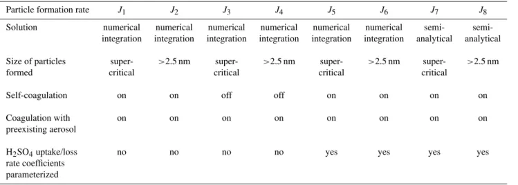
Table 1.Details of the steady state particle formation rate calculations.
Particle formation rate J1 J2 J3 J4 J5 J6 J7 J8
Solution numerical numerical numerical numerical numerical numerical semi- semi-integration integration integration integration integration integration analytical analytical
Size of particles super- >2.5 nm super- >2.5 nm super- >2.5 nm super- >2.5 nm
formed critical critical critical critical
Self-coagulation on on off off on on on on
Coagulation with on on on on on on on on
preexisting aerosol
H2SO4uptake/loss no no no no yes yes yes yes
rate coefficients parameterized
rates can in general be neglected in the context of atmo-spheric aerosol formation. The particle formation rates are sampled on a grid of parameters covering the inter-vals[2,35]cm−3s−1 (ionization rate q), [25,104]% (rela-tive humidity r), [0,0.01]s−1 (preexisting aerosol H2SO4
condensational sink s), [190,285]K (temperature t), and [106,2×10⁸]cm−3 (sulfuric acid gas phase concentration [H2SO4]), with 7 equidistant grid points on each interval.
While this parameter grid covers typical tropospheric condi-tions, the resulting samples will produce an incomplete pic-ture of the differences between the particle formation rates: The extent and resolution of the grid introduce a sampling uncertainty. Moreover, the deviations between the particle formation rates are not a representative measure of their per-formance when used in an atmospheric model, as the joint probability distribution of the parameters controlling aerosol formation needs not to be uniform in the atmosphere.
Relative humidities below 25%, sulfuric acid concentra-tions below 106cm−3, and temperatures above 285 K were excluded from the comparison: The numerical model de-scribed in Sect. 8 is unable reach the steady state criterion for unfavorable combinations of these parameters, when the par-ticle formation rates are extremely small (≪10−6cm−3s−1), possibly due to numerical errors. The pressure p is set to 1013.25 hPa in all calculations, as the considered parti-cles are much smaller than the mean free path of gas phase molecules, and their processes take place in the free molecu-lar regime, with a negligible pressure dependence.
9.1 Nucleation rate as a surrogate for the formation rate of particles of a given size
In large scale atmospheric models treating sulfate aerosol, particle formation rates are usually calculated with nucle-ation rate parameteriznucle-ations. The smallest represented
par-ticles in these models (e.g. Lauer et al., 2005; Ma and von Salzen, 2006) may be larger (2–10 nm) than the neutral criti-cal cluster, which contains only a few sulfuric acid molecules in conditions favorable for nucleation. The loss of supercrit-ical particles smaller than the smallest represented particles due to coagulation among each other and with larger aerosol is then neglected, leading to an overestimation of particle for-mation rates. The resulting errors add to the intrinsic errors of aerosol nucleation parameterizations, which may exceed a factor of 2 (Vehkam¨aki et al., 2002; Modgil et al., 2005).
10
-610
-410
-210
010
210
410
6J
2(cm
-3s
-1)
10
010
210
410
6J
1/J
2(
a
)
2⋅106 cm-3
3.5⋅10
7 cm-3 6.8⋅107 cm-3
1⋅108 cm-3
1.3⋅108 cm-3
1.7⋅108 cm-3
2⋅108 cm-3 [H2SO4] :
10
-610
-410
-210
010
210
410
6J
2(cm
-3s
-1)
10
010
210
410
6(d’/D’)
1/3
J
1/J
2(
b
)
2⋅106 cm-3
3.5⋅107 cm-3
6.8⋅107 cm-3
1⋅108 cm-3
1.3⋅108 cm-3
1.7⋅108 cm-3
2⋅108 cm-3
[H2SO4] :
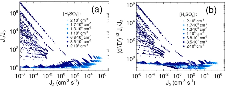
Fig. 4. (a)Comparison of the nucleation rateJ1with the formation rateJ2of particles exceeding 2.5 nm in diameter.(b)Comparison of the nucleation rateJ1, scaled with the factor(d′/D′)3, with the formation rateJ2of particles exceeding 2.5 nm in diameter.d′is the diameter of the smallest supercritical particle in given conditions,D′the diameter of the smallest particle exceeding 2.5 nm. The particle formation rate calculations are described in more detail in Table 1.
In both cases (Figs. 4a and b) the largest differences be-tween the nucleation rate and the>2.5 nm particle forma-tion rate occur at the lowest H2SO4concentrations and at the
lowest temperatures (not shown). This can be explained as follows: At very low temperatures the neutral critical cluster contains very few H2SO4molecules, and even comparably
low H2SO4concentrations can sustain non-negligible
nucle-ation rates. However, at low H2SO4concentrations, particles
grow slowly, and a given nucleation rate may result in a much smaller formation rate of>2.5 nm particles, owing to loss of particles due to coagulation among each other and with pre-existing aerosol.
9.2 Self-coagulation and particle formation
Kerminen and Kulmala (2002) have developed an analytical method to calculate the formation rate of particles of a given size from the formation rate of particles of a smaller size. The method accounts for coagulation with preexisting aerosol, but neglects self-coagulation. Self-coagulation is the coagu-lation of the forming particles among each other, as opposed to coagulation with preexisting, typically larger aerosol par-ticles. Unlike coagulation with preexisting aerosol, self-coagulation acts not only as a particle sink, but also con-tributes to the formation of new particles.
Figure 5a compares the nucleation rate calculated with and without self-coagulation of the nucleating particles. 99% of the nucleation rates calculated without self-coagulation lie within 29% of the nucleation rates calculated with self-coagulation. Figure 5b shows the errors encountered when calculating the formation rate of particles exceeding 2.5 nm in diameter without self-coagulation: Here, 31% of the
parti-cle formation rates calculated without self-coagulation devi-ate 99% or more from the particle formation rdevi-ates calculdevi-ated with self-coagulation. In both cases the largest deviations occur at the low end of the considered temperature range (≤206 K for the nucleation and≤238 K for the>2.5 nm par-ticle formation rate). Hence neglecting self-coagulation is a reasonable approximation in the calculation of the steady state formation rate for small particles or at sufficiently high temperatures.
9.3 Semi-analytical versus numerical particle formation rate calculation
Here we compare the particle formation rates calculated with the semi-analytical method (described in Sect. 7) with par-ticle formation rates calculated with the numerical aerosol model (described in Sect. 8). Both methods employ parame-terized H2SO4uptake and loss rate coefficients and average
particle H2O contents (Sect. 6). The rate coefficients for
co-agulation of the particles among each other and with preex-isting aerosol are calculated as described in Sect. 4.
Figure 6a shows the relative deviations of the semi-analytical nucleation rates with respect to the numerical nu-cleation rates. The deviations are minuscule: The maximum error amounts to 0.41%. Figure 6b shows the relative devi-ation of the semi-analytical formdevi-ation rates of particles ex-ceeding 2.5 nm in diameter with respect to the correspond-ing numerical particle formation rates. These deviations are small: The maximum error amounts to 2.0%.
10
-610
-410
-210
010
210
410
6J
1(cm
-3s
-1)
-35
-30
-25
-20
-15
-10
-5
0
5
10
15
(J
3-J
1)/J
1
(%)
(
a
)
190 K 206 K 222 K 238 K 253 K 269 K 285 K
Temperature :
10
-610
-410
-210
010
210
410
6J
2(cm
-3s
-1)
0.1
1.0
10.0
J
4/J
2(b)
190 K 206 K 222 K 238 K 253 K 269 K 285 K
Temperature :
Fig. 5. (a)Comparison of the nucleation rateJ3, calculated with self-coagulation of the nucleating particles switched off, with the nucleation rateJ1, calculated with self-coagulation acting both as a particle sink as well as a contribution to the nucleation rate. (b)Comparison of the formation rateJ4of particles exceeding 2.5 nm in diameter, calculated with self-coagulation switched off, with the formation rateJ2of particles exceeding 2.5 nm in diameter, calculated with self-coagulation acting both as a particle sink as well as a contribution to the particle formation rate. The particle formation rate calculations are described in more detail in Table 1.
10
-610
-410
-210
010
210
410
6J
5(cm
-3s
-1)
-0.1
0.0
0.1
0.2
0.3
0.4
0.5
(J
7-J
5)/J
5
(%)
(
a
)
2⋅106 cm-3
3.5⋅107 cm-3
6.8⋅107 cm-3
1⋅108 cm-3
1.3⋅108 cm-3
1.7⋅108 cm-3
2⋅108 cm-3 [H2SO4] :
10
-610
-410
-210
010
210
410
6J
6(cm
-3s
-1)
-2.0
-1.5
-1.0
-0.5
0.0
0.5
(J
8-J
6)/J
6
(%)
(
b
)
2⋅106 cm-3
3.5⋅107 cm-3
6.8⋅107 cm-3
1⋅108 cm-3
1.3⋅108 cm-3
1.7⋅108 cm-3
2⋅108 cm-3
[H2SO4] :
Fig. 6. (a)Comparison of the nucleation rateJ7, calculated with our semi-analytical method, with the nucleation rateJ5calculated with a numerical aerosol model.(b)Comparison of the formation rateJ8of aerosol particles exceeding 2.5 nm in diameter, calculated with our semi-analytical method, with the particle formation rateJ6of particles exceeding 2.5 nm in diameter, calculated with a numerical aerosol model. Here, both the semi-analytical method and the numerical model use parameterized rate coefficients for the uptake and loss of H2SO4 by the aerosol particles, as well as parameterized average particle H2O contents. The particle formation rate calculations are described in more detail in Table 1.
>2.5 nm particle formation rates. A further acceleration can be achieved when requirements on precision are relaxed, e.g. by reducing the number of iterations in the semi-analytical method. The time for calculating the rate coefficients has been excluded from this comparison.
9.4 Semi-analytical particle formation rates using parame-terized rate coefficients versus numerical particle for-mation rates using calculated rate coefficients
10
-610
-410
-210
010
210
410
6J
1(cm
-3s
-1)
-5
0
5
10
15
20
(J
7-J
1)/J
1
(%)
(
a
)
2⋅10
6
cm-3 3.5⋅107 cm-3
6.8⋅107 cm-3
1⋅108 cm-3
1.3⋅108 cm-3
1.7⋅10
8
cm-3 2⋅108 cm-3
[H2SO4] :
10
-610
-410
-210
010
210
410
6J
2(cm
-3s
-1)
-5
0
5
10
15
20
(J
8-J
2)/J
2
(%)
(
b
)
2⋅106 cm-3
3.5⋅107 cm-3
6.8⋅107 cm-3
1⋅10
8
cm-3
1.3⋅108 cm-3
1.7⋅108 cm-3
2⋅108 cm-3
[H2SO4] :
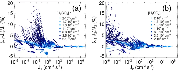
Fig. 7. (a)Comparison of the nucleation rateJ7, calculated with our semi-analytical method, with the nucleation rateJ1, calculated with a numerical aerosol model.(b)Comparison of the formation rateJ8of aerosol particles exceeding 2.5 nm in diameter, calculated with our semi-analytical method, with the particle formation rateJ2, calculated with a numerical aerosol model. The semi-analytical method uses parameterized rate coefficients for the uptake and loss of H2SO4by the aerosol particles and parameterized average particle H2O contents, while the numerical model calculates the rate coefficients and average particle H2O contents from scratch. The particle formation rate calculations are described in more detail in Table 1.
H2O contents (Sect. 6), with particle formation rates
calcu-lated with the numerical aerosol model described in Sect. 8, which uses H2SO4 uptake and loss rate coefficients and
and average particle H2O contents calculated from scratch
(Sect. 4). The rate coefficients for coagulation of the particles among each other and with preexisting aerosol are calculated as described in Sect. 4 by both methods.
Figure 7a shows the relative deviation of the semi-analytical nucleation rates with respect to the numerical nu-cleation rates. The maximum error amounts to 18%. Larger deviations are possible (but do not appear on the used pa-rameter grid) when errors in the papa-rameterized rate coeffi-cients lead to an erroneous determination of the neutral crit-ical cluster H2SO4content. Figure 7b shows the relative
de-viation of the semi-analytical formation rates of particles ex-ceeding 2.5 nm in diameter with respect to the corresponding numerical particle formation rates. Here the maximum error amounts to 20%. In both cases, the deviations are mainly due to errors in the parameterization of the rate coefficients for uptake and loss of H2SO4by the aerosol particles.
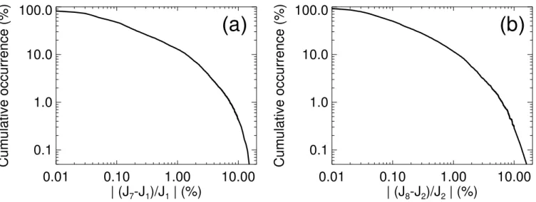
Figure 8 shows the cumulative error occurrence (fraction of errors exceeding a given value) of the semi-analytical par-ticle formation rates with respect to the numerical parpar-ticle formation rates. For both the semi-analytical nucleation rate and the>2.5 nm particle formation rate the cumulative error occurrence falls off quickly, signifying the rare occurrence of large deviations. The cumulative error occurrences are based on particular samples of particle formation rates, and are therefore subject to a sampling uncertainty.
The semi-analytical method using parameterized rate co-efficients and average particle water contents is faster than the numerical model using rate coefficients and average par-ticle water contents calculated from scratch when run for a time period of 1200 s by a factor of several hundred in the case of the>2.5 nm particle formation rates. A further accel-eration can be achieved when requirements on precision are relaxed, e.g. by reducing the number of iterations in the semi-analytical method, or the maximum order of the Chebyshev polynomial expansion used in the rate coefficient parameter-ization.
10 Summary, discussion, and outlook
Secondary aerosol formation can significantly increase the concentrations of aerosol particles and cloud condensation nuclei in the atmosphere, and therefore requires dependable representations in atmospheric models. However, available representations reproduce aerosol nucleation rates calculated with detailed numerical models only imprecisely. In addi-tion, substantial errors, exceeding an order of magnitude in some cases, can arise when the steady state nucleation rate is used as a surrogate for the steady state formation rate of particles of a given size. To overcome these limitations we have developed a new, semi-analytical method to calculate secondary aerosol formation rates in steady state. The ad-vantages of our method are:
0.01
0.10
1.00
10.00
| (J
7-J
1)/J
1| (%)
0.1
1.0
10.0
100.0
Cumulative occurrence (%)
(
a
)
0.01
0.10
1.00
10.00
| (J
8-J
2)/J
2| (%)
0.1
1.0
10.0
100.0
Cumulative occurrence (%)
(
b
)
Fig. 8.Cumulative error occurrence (fraction of errors exceeding a given value) of particle formation rates calculated with our semi-analytical method, relative to the particle formation rates calculated with a numerical aerosol model:(a)nucleation rate,(b)formation rate of particles exceeding 2.5 nm in diameter. See Table 1 for details of the particle formation rate calculations.
– its detailed representation of the physical processes leading to new aerosol formation,
– its ability to calculate nucleation rates as well as the for-mation rates of particles of a given size,
– the good agreement of the resulting particle forma-tion rates with those calculated by a numerical aerosol model.
Disadvantages of our method include
– its higher complexity compared to aerosol formation rate parameterizations, resulting in a higher numerical cost,
– the limited number of aerosol formation mechanisms accounted for: Potentially important mechanisms such as ternary nucleation of ammonia, sulfuric acid, and wa-ter, or nucleation involving organic molecules are not included.
How do we proceed from here with respect to representing aerosol formation from the gas phase in atmospheric mod-eling? Let us muse about possible developments that may advance the field:
First of all, a procedure for assessing and evaluating the various available and future aerosol formation representa-tions needs to be devised. Simply comparing the output of the different representations is not enough: On the one hand, none of the methods can be considered a standard a priori. On the other hand, the flaws in a given representation may not matter when it is used in an atmospheric model: As an example, the joint probability distribution of the parameters controlling aerosol formation needs not to be uniform in the
atmosphere. Then errors of a representation would matter lit-tle if they were confined to conditions that occur infrequently, or that contribute little to overall aerosol production. Conse-quently, assessing and evaluating different implementations should be done using an atmospheric model and comparing its output to observations. In this, it should be noted that large scale models often rely on highly simplified representa-tions of many processes and have a limited spatial resolution. Large scale models may therefore produce good results with a relatively simple but efficient representation of aerosol for-mation. Smaller scale models, which resolve many processes in detail and on smaller spatial scales may require more so-phisticated representations of aerosol formation to produce a good agreement of model results and observations.
The question when steady state representations of aerosol formation are indeed applicable should be addressed: Vig-orous nucleation events for example, such as observed in the upper troposphere in connection with tropical convection may not be well captured by steady state methods.
also be accelerated by finding algorithms that reduce the number of iterations required for convergence towards steady state. Another promising approach for representing aerosol formation rates that has not been widely explored yet is the interpolation of lookup tables.
However, the most severe limitation on modeling sec-ondary aerosol formation in the atmosphere is our lack of understanding of the processes that lead to the formation of stable molecular clusters from the gas phase. Labora-tory studies investigating the structure of such clusters and measuring their thermodynamic formation parameters have therefore the greatest potential to advance the field.
11 Conclusions
Secondary aerosol formation can significantly increase con-centrations of aerosol particles and cloud condensation nu-clei in the atmosphere, and therefore requires dependable representations in atmospheric models. However, the avail-able representations reproduce aerosol nucleation rates cal-culated with detailed numerical models only imprecisely. In addition, substantial errors, exceeding an order of magnitude in some cases, can arise when the steady state nucleation rate is used as a surrogate for the steady state formation rate of particles of a given size. To overcome these limitations, we have developed a semi-analytical method to calculate steady state formation rates of sulfate aerosol which uses parameter-ized rate coefficients for sulfuric acid uptake and loss by the aerosol particles. The method reproduces aerosol formation rates calculated with a numerical aerosol model better than other available methods, but is numerically more complex. The method can calculate the steady state formation rates of particles of a given size, and therefore supersedes the use of nucleation rates in lieu of formation rates of larger particles.
Acknowledgements. We thank S. L. Clegg (University of East Anglia) for providing the computer code for calculating activities of sulfuric acid/water solutions. This work was performed while the first author held a National Research Council Research Asso-ciateship Award, and was supported by the NOAA Climate and Global Change Program.
Edited by: M. Kulmala
References
Allan, J. D., Alfarra, M. R., Bower, K. N., Coe, H., Jayne, J. T., Worsnop, D. R., Aalto, P. P., Kulmala, M., Hy¨otyl¨ainen, T., Cav-alli, F., and Laaksonen, A.: Size and composition measurements of background aerosol and new particle growth in a Finnish forest during QUEST 2 using an Aerodyne Aerosol Mass Spectrome-ter, Atmos. Chem. Phys., 6, 315–327, 2006,
http://www.atmos-chem-phys.net/6/315/2006/.
Bates, D. R.: Recombination of small ions in the troposphere and lower stratosphere, Planet. Space Sci., 30, 1275–1282, 1982.
Brock, C. A., Hamill, P., Wilson, J. C., Jonsson, H. H., and Chan, K. R.: Particle formation in the upper tropical troposphere: a source of nuclei for the stratospheric aerosol, Science, 270, 1650–1653, 1995.
Cavalli, F., Facchini, M. C., Decesari, S., Emblico, L., Mircea, M., Jensen, N. R., and Fuzzi, S.: Size-segregated aerosol chemi-cal composition at a boreal site in southern Finland, during the QUEST project, Atmos. Chem. Phys., 6, 993–1002, 2006, http://www.atmos-chem-phys.net/6/993/2006/.
Clarke, A. D.: Atmospheric nuclei in the remote free-troposphere, J. Atmos. Chem., 14, 479–488, 1992.
Clegg, S. L., Rard, J. A., and Pitzer, K. S.: Thermodynamic prop-erties of 0–6 mol kg−1 aqueous sulfuric acid from 273.15 to 328.15 K, J. Chem. Soc., Faraday Trans., 90, 1875–1894, doi: 10.1039/FT9949001875, 1994.
Coffman, D. J. and Hegg, D. A.: A preliminary study of the effect of ammonia on particle nucleation in the marine boundary layer, J. Geophys. Res., 100, 7147–7160, doi:10.1029/94JD03253, 1995. Curtius, J., Froyd, K. D., and Lovejoy, E. R.: Cluster ion thermal decomposition (I): Experimental kinetics study and ab initio cal-culations for HSO−4(H2SO4)(x)(HNO3)(y), J. Phys. Chem. A, 105, 10 867–10 873, 2001.
Froyd, K. D.: Ion induced nucleation in the atmosphere: Studies of NH3, H2SO4, and H2O cluster ions, Ph.D. thesis, Univ. of Colo., Boulder, 2002.
Froyd, K. D. and Lovejoy, E. R.: Experimental Thermodynamics of Cluster Ions Composed of H2SO4and H2O. 1. Positive Ions, J. Phys. Chem. A, 107, 9800–9811, 2003a.
Froyd, K. D. and Lovejoy, E. R.: Experimental Thermodynamics of Cluster Ions Composed of H2SO4and H2O. 2. Measurements and ab Initio Structures of Negative Ions, J. Phys. Chem. A, 107, 9812–9824, 2003b.
Fuchs, N. A.: The Mechanics of Aerosols, Macmillan, 1964. Giauque, W. F., Hornung, E. W., Kunzler, J. E., and Rubin, T. T.:
The thermodynamic properties of aqueous sulfuric acid solutions and hydrates from 15 to 300 K, Am. Chem. Soc. J., 82, 62–70, 1960.
Goff, J. A.: Saturation pressure of water on the new Kelvin temper-ature scale, in: Transactions of the American Society of Heat-ing and VentilatHeat-ing Engineers, pp. 347–354, American Society of Heating and Ventilating Engineers, 1957.
Hanson, D. R. and Lovejoy, E. R.: Measurement of the thermody-namics of the hydrated dimer and trimer of sulfuric acid, J. Phys. Chem. A, 110, 9525–9528, doi:10.1021/jp062844w, 2006. Haywood, J. and Boucher, O.: Estimates of the direct and indirect
radiative forcing due to tropospheric aerosols: A review, Rev. Geophys., 38, 513–543, doi:10.1029/1999RG000078, 2000. Heintzenberg, J.: Fine particles in the global troposphere, Tellus
Series B Chemical and Physical Meteorology B, 41, 149–160, 1989.
Heintzenberg, J., Covert, D. S., and Van Dingenen, R.: Size distri-bution and chemical composition of marine aerosols: A compi-lation and review, Tellus, 52B, 1104–1122, 2000.
Jacobson, M. C., Hansson, H.-C., Noone, K. J., and Charlson, R. J.: Organic atmospheric aerosols: Review and state of the sci-ence, Rev. Geophys., 38, 267–294, doi:10.1029/1998RG000045, 2000.
2007.
Kerminen, V.-M. and Kulmala, M.: Analytical formulae connecting the “real” and the “apparent” nucleation rate and the nuclei num-ber concentration for atmospheric nucleation events, J. Aerosol Sci., 33, 609–622, doi:10.1016/S0021-8502(01)00194-X, 2002. Kulmala, M., Vehkam¨aki, H., Pet¨aj¨a, T., Dal Maso, M., Lauri, A., Kerminen, V.-M., Birmili, W., and McMurry, P. H.: Formation and growth rates of ultrafine atmospheric particles: A review of observations, J. Aer. Sci., 35, 143–176, doi:10.1016/j.jaerosci. 2003.10.003, 2004a.
Kulmala, M., Kerminen, V.-M., Anttila, T., Laaksonen, A., and O’Dowd, C. D.: Organic aerosol formation via sulphate clus-ter activation, J. Geophys. Res., 109, D4205, doi:10.1029/ 2003JD003961, 2004b.
Lauer, A., Hendricks, J., Ackermann, I., Schell, B., Hass, H., and Metzger, S.: Simulating aerosol microphysics with the ECHAM/MADE GCM – Part I: Model description and compari-son with observations, Atmos. Chem. Phys., 5, 3251–3276, 2005, http://www.atmos-chem-phys.net/5/3251/2005/.
Lehtinen, K. E. J. and Kulmala, M.: A model for particle formation and growth in the atmosphere with molecular resolution in size, Atmos. Chem. Phys., 3, 251–258, 2003,
http://www.atmos-chem-phys.net/3/251/2003/.
Lohmann, U. and Feichter, J.: Global indirect aerosol effects: a review, Atmos. Chem. Phys., 5, 715–737, 2005,
http://www.atmos-chem-phys.net/5/715/2005/.
Lovejoy, E. R., Curtius, J., and Froyd, K. D.: Atmospheric ion-induced nucleation of sulfuric acid and water, J. Geophys. Res., 109, D08204, doi:10.1029/2003JD004460, 2004.
Ma, X. and von Salzen, K.: Dynamics of the sulphate aerosol size distribution on a global scale, J. Geophys. Res., 111, D08 206, doi:10.1029/2005JD006620, 2006.
Modgil, M. S., Kumar, S., Tripathi, S. N., and Lovejoy, E. R.: A parameterization of ion-induced nucleation of sulphuric acid and water for atmospheric conditions, J. Geophys. Res., 110, D19205, doi:10.1029/2004JD005475, 2005.
Napari, I., Noppel, M., Vehkam¨aki, H., and Kulmala, M.: Parametrization of ternary nucleation rates for H2SO4-NH3 -H2O vapors, J. Geophys. Res., 107, 6–1, doi:10.1029/ 2002JD002132, 2002.
Ravishankara, A. R.: Heterogeneous and Multiphase Chemistry in the Troposphere, Science, 276, 1058–1065, doi:10.1126/science. 276.5315.1058, 1997.
Smith, J. N., Moore, K. F., Eisele, F. L., Voisin, D., Ghimire, A. K., Sakurai, H., and McMurry, P. H.: Chemical composition of atmospheric nanoparticles during nucleation events in Atlanta, J. Geophys. Res., 110, D22S03, doi:10.1029/2005JD005912, 2005.