a onshore wind turbine
Dissertação para obtenção do Grau de Mestre em Engenharia Civil
Orientador:
, Senior Advisor, Deltares
Co-orientador:
, Professor Auxiliar,
FCT/UNL
Júri:
Presidente: Prof. Doutor Carlos Chastre Rodrigues Arguente: Prof. Doutor João Bilé Serra
Vogal: Prof. Doutor José Nuno Varandas
and concern that I could ever expect. I am very grateful for all the knowledge you shared with me and for all the critical comments that helped improving my master thesis. I thank professor Jos´e Varandas for all the help and guidance. This thesis was never possible if there was not for the effort, patience and dedication shown during the process. Thank you very much for being always available for discussion and ready to give insightful advices. To both, from the bottom of my heart, I thank you for the friendship. I will always keep with me what you thought me and I am very grateful for your presence in my last step as an engineering student. I feel privileged to have had the opportunity to work with both of you.
Finally, I thank my family, friends and loved ones. All of you gave me extraordinary support in this chapter of my life and I believe if university was crucial for my development as civil engineer, you gave me the best self development i could ever wish. It wouldn’t be possible to finish this chapter of my life if there wasn’t for all the love, care, laughs and support i had. To all, I will always keep you in my heart.
To the phenomenon of interaction between two piles and the soil between them it’s given the name of pile-soil-pile interaction. It is known that such behavior is frequency de-pendent, and therefore, on this work evaluation of relevant frequencies for the intended analysis is held. During the development of this thesis, two methods were selected in order to assess pile-soil-pile interaction, being one of analytical nature and the other of numerical origin. The analytical solution was recently developed and its called Gener-alized pile-soil-pile theory, while for the numerical method the commercial finite element software PLAXIS 3D was used. A study of applicability of the numerical method is also done comparing the given solution by the finite element methods with a rigorous solution widely accepted by the majority of the authors.
Keywords: Dynamic Stiffness; Pile-soil-pile interaction; Wind turbines; FAST; PLAXIS 3D
uma funda¸c˜ao que esteja assente num dique.
Ao fen´omeno de interac¸c˜ao entre duas estacas e o solo entre estas, d´a-se o nome de in-terac¸c˜ao estaca-solo-estaca. ´E sabido que tal comportamento ´e dependente da frequˆencia de excita¸c˜ao e, sendo assim, neste trabalho procede-se tamb´em `a avalia¸c˜ao das frequˆencias relevantes para a an´alise em quest˜ao. Durante o desenvolvimento desta tese, dois m´etodos s˜ao seleccionados para estudar a interac¸c˜ao estaca-solo-estaca, sendo um de natureza anal´ıtica e outro de origem num´erica. A solu¸c˜ao anal´ıtica foi recentemente desenvolvida e ´e denominada de Generalized pile-soil-pile theory, enquanto que para a an´alise num´erica recorre-se aosoftware comercial de elementos finitos PLAXIS 3D. ´E ainda efectuada um estudo de aplicabilidade do m´etodo num´erico para este tipo de problemas procedendo `a compara¸c˜ao da solu¸c˜ao obtida pelo m´etodo dos elementos finitos com uma solu¸c˜ao rigorosa vastamente aceite pela maioria dos autores.
Palavras chave: Rigidez dinˆamica; Intera¸c˜ao estaca-solo-estaca; Turbinas e´olicas; FAST; PLAXIS 3D
2 Problem Description 5
3 Wind-Turbine Interaction Analysis 13
3.1 Introduction . . . 13
3.2 FAST - Fatigue, Aerodynamics, Structures and Turbulence . . . 13
3.2.1 Generation of wind field . . . 17
3.2.2 AeroDyn . . . 18
3.3 Model Parametrization . . . 20
3.3.1 Wind Turbine Model . . . 20
3.3.2 Wind Model . . . 22
3.3.3 AeroDyn Model . . . 26
3.3.4 FAST Model . . . 26
3.4 Numerical Simulation . . . 28
3.4.1 Wind Speeds . . . 29
3.4.2 Loads on wind turbine base . . . 29
3.5 Discussion . . . 32
3.6 Conclusions . . . 33
4 Geotechnical and Foundation Model 37 4.1 Introduction . . . 37
4.2 Soil Characterization . . . 37
4.2.2 Data interpretation . . . 39
4.2.3 Layer definition and obtained results . . . 44
4.2.4 Adopted Soil Parameters . . . 47
4.3 Foundation Preliminary Design . . . 52
4.3.1 Adopted foundation Loads . . . 52
4.3.2 Pile capacity for axial loading . . . 55
4.3.3 Final foundation model . . . 57
4.4 Conclusions . . . 58
5 Pile-Soil-Pile Interaction 59 5.1 Introduction . . . 59
5.2 Generalized Pile-Soil-Pile Theory . . . 59
5.2.1 Vertical Stiffness . . . 62
5.2.2 Horizontal Stiffness . . . 63
5.2.3 Rocking Stiffness . . . 64
5.2.4 Analytical results . . . 65
5.3 3D Numerical Solution . . . 68
5.3.1 Numerical aspects in PLAXIS . . . 68
5.3.2 PLAXIS model . . . 72
5.3.2.1 Soil definition . . . 72
5.3.2.2 Adopted geometry . . . 73
5.3.2.3 Structural model . . . 73
5.3.2.4 Mesh . . . 75
5.3.2.5 Staged construction . . . 76
5.3.2.6 Output model . . . 78
5.4 Results and discussion . . . 80
5.5 Conclusions . . . 84
6 Conclusions and Future Developments 85 6.1 Conclusions . . . 85
6.2 Future Developments . . . 86
Bibliography 88 A Natural frequency calculation using Rayleigh-Ritz analysis 93 B FAST, TurbSim and AeroDyn input files 97 B.1 FAST input file . . . 97
B.2 TurbSim input file . . . 103
B.3 AeroDyn input file . . . 106
3.5 Example of a grid and the coordinate system used in TurbSim, Jonkman
and Kilcher (2012) . . . 18
3.6 Generator power output during pitch change, Moriarty and Hansen (2005) . 20 3.7 Structural model of a flexible wind turbine system, van der Tempel and Molenaar (2002) . . . 23
3.8 1P and 3P intervals and natural frequency plot for NREL 5-MW Baseline wind turbine . . . 23
3.9 Maximum windspeed measured in Lauwersoog weather station over 15552 days . . . 25
3.10 Wind speed in xt(a),yt(b) andzt(c) directions . . . 29
3.11 Tower base shear forces directed alongxt(a), yt(b) andzt(c) direction . . . 30
3.12 Tower base moment around xt(a), yt(b) and zt(c) axis . . . 31
3.13 Rotor angular speed over the simulated time . . . 31
3.14 Amplitude spectrum of the wind turbine’s response calculated using fast Fourier transforms inxt(a), yt(b) andzt(c) directions . . . 34
3.15 Amplitude spectrum of the wind action calculated using fast Fourier trans-forms inxt(a), yt(b) andzt(c) directions . . . 34
4.1 Schematic profile of the geotechnical model being defined . . . 38
4.2 Local of CPT testing, taken from Google Earth version 7.1.2.2041 . . . 39
4.3 Measured field data from CPT S02G00190 . . . 40
4.4 Normalized CPT soil behavior type chart, Robertson (2010) . . . 42
4.5 Soil behaviour type index ploted over elevation for CPT S02G00190 . . . . 43
4.7 Continuous plot of soil behavior type index for all CPTs executed . . . 46
4.8 Plotted results for the total unit weight on each layer . . . 48
4.9 Plotted results for the angle of friction on first and third soil layer . . . 49
4.10 Plotted results for undrained shear strength on the second layer layer . . . 49
4.11 Plotted results for the elastic modulus on all soil layers . . . 50
4.12 Mechanical diagram of the soil medium . . . 51
4.13 Two-dimensional force diagram of the foundation . . . 53
4.14 Two possible scenarios for vertical loading due to cap rotation . . . 56
5.1 Results for vertical group stiffness(a) and damping(b) coefficients . . . 66
5.2 Results for horizontal group stiffness(a) and damping(b) coefficients . . . . 67
5.3 Results for rocking group stiffness(a) and damping(b) coefficients . . . 67
5.4 10-node tetrahedral element used in PLAXIS 3D . . . 70
5.5 Adopted model dimensions in PLAXIS simulation . . . 73
5.6 Embedded pile model, adapted from Brinkgreve et al. (2013) . . . 75
5.7 Adopted mesh for f = 1.2 Hz . . . 76
5.8 Cap displacement over time for a group of 24 piles loaded at a frequency of 0.3 Hz . . . 79
5.9 Normalized curves for force and displacement from whereϕ is read . . . 80
5.10 Vertical group stiffness(a) and damping(b) coefficients calculated using PLAXIS 81 5.11 Horizontal group stiffness(a) and damping(b) coefficients calculated using PLAXIS . . . 81
5.12 Rocking group stiffness(a) and damping(b) coefficients calculated using PLAXIS . . . 81
5.2 Adopted soil parameters in PLAXIS . . . 73
5.3 Adopted plate and embedded pile parameters . . . 74
5.4 Influence evaluation of the the element size around the piles . . . 76
5.5 Adopted average element size . . . 76
5.6 Dynamic time . . . 77
5.7 Evaluation of the induced error by time step . . . 78 5.8 Analyzed dimensionless frequencies and corresponding liner frequency values 83
c Damping coefficient
c′
Soil cohesion
C1,C2 Relaxation coefficients Cd Damping coefficient
cp Soil compression wave velocity
cLA Lysmer’s analog velocity
cs Soil shear wave velocity
cvg,chg,cθg Vertical, horizontal and bending damping coefficients of the pile group
CzG Vertical Damping coefficient of a group of piles
d Plate element thickness
Df Foundation cap diameter
Dp Pile diameter
E Soil deformation modulus
Ep Pile deformation modulus
F Generic force ˆ
F Force amplitude
f Linear frequency
FG Vertical forces applied on the foundation cap
Fj Force acting on pilej
FM Additional total vertical force on the cap due to the bending moment FM;max Additional maximum vertical force on a single pile due to the bending
moment
Fmax Embedded pile foot resistance
Fr Normalized friction ratio fs Sleeve friction
Fvert Vertical force on all piles
Fvp Maximum total vertical load on a pile
G Soil shear modulus
Ic Soil behavior type index
K Stiffness matrix
K Lateral earth pressure coefficient
k Stiffness coefficient
K0 Lateral earth pressure coefficient ”at-rest‘ Kd Dynamic stiffness of a single pile
Kd Dynamic stiffness coefficient
kn,kt Elastic normal stiffness of the embedded pile element
ks Elastic shear stiffness of the embedded pile Kvg Vertical dynamic stiffness of a group of piles
kvg,khg,kθg Vertical, horizontal and bending stiffness coefficients of the pile group KGz Vertical dynamic stiffness coefficient of a group of piles
Kzs Static stiffness of a single pile
le Average finite element size
lp Pile length
M Mass matrix
Rb Pile tip resistance
re Relative finite element size factor R Foundation radius
Rf Friction ratio Rs Pile shaft resistance
s/d Dimensionless pile spacing
su Undrained shear strength
t Time
tc Foundation cap thickness
ttotal Total calculation time
Tmax Embedded pile skin resistance per meter ˆ
u Displacement amplitude
uz Vertical cap displacement
Vx,Vy Shear force inx and y directions
Wcap Foundation cap weight
wi Displacement of pile i
Greek Symbols
α Dimensionless adhesion coefficient
αr Rayleigh coefficient for mass influence in the damping of the system
αs Static interaction factor β Soil damping ratio
βr Rayleigh coefficient for stiffness influence in the damping of the system
γ,γt Total unit weight
γw Water unit weight
δ Soil-structure friction angle ∆ij Spacing between pileiand pilej
∆t Time step
δt Time difference between excitation and response θij Angle between pile iandj
θj Angle between pile j and the foundation center
λ Wavelength
ν Poisson ratio
ξ Damping ratio
ρ Material density
σn Normal stress
σ′
v Mean vertical effective stress along pile shaft σ′
v0,σ ′
0 Vertical stress τ Shear stress
φ Foundation cap rotation
φ′
Soil friction angle
φ0 Initial phase angle ϕ Phase angle
after the oil crisis in the mid 1970’s, renewable energies have been a matter of study and development, with wind energy leading the way to achieve reliable, effective and clean energy. Wind turbines are nowadays an usual element on the landscape of many European countries (Castro, 2009). Among Germany, Denmark or the USA, The Netherlands has been one of the countries that deposits high expectations on this technology with extensive experience on both off-shore and on-shore wind turbines.
2 Introduction
1.2
Aim of research
The aim of the present thesis is to properly evaluate the dynamic loads caused by a wind turbine on its foundation which is composed by a piled group and the computation of the dynamic stiffness, estimating both the stiffness and damping coefficients. This problem is approached using two different methods. An analytical method called general pile-soil-pile interaction developed by H¨olscher (2014a) and a numerical approach using a finite element analysis using the software PLAXIS 3D. Also, it is investigated the applicability of the finite element approach to this type of problems and if the method is capable of describing the pile-soil-pile interaction in terms of value and trend. The analysis is based on real scenario data, more precisely, the investigation is made for a potential implementation of a wind turbine mounted on a dike located in Lauwersoog, The Netherlands.
1.3
Outline of the Thesis
Chapter 2 starts by introducing the phenomenon of pile-soil-pile interaction. A brief de-scription of the work made so far on pile group interaction is made showing the differences between the static and dynamic behavior of a piled foundation. The main conclusions on previous studies on dynamic soil-structure interaction is presented where is clear the frequency dependent behavior of this type of foundation.
In chapter 3, wind turbine behavior is studied. The wind action is described using real wind data from a weather station. The computation of the dynamic wind loads is made using the software FAST where the plotted results are three dimensional time series of loads on every direction. Also, the evaluation of the natural frequency of the wind turbine is made as well as the response frequencies of the system.
After the calculation of wind loads on the base of the tower, Chapter 4 defines the miss-ing variables in order to perform a pile-soil-pile interaction analysis. Here a geotechnical model is built by first characterizing the soil medium, using cone penetration tests. Af-ter, a foundation preliminary design was held using the computed loads on the previous chapter. This foundation preliminary design was made using to Eurocode 7 specification and respecting its safety requirements.
a group of piles connected by a concrete cap.
Many engineering models simplify the problem by considering that the soil-structure model is represented by a spring-dashpot system as schematized in Figure 2.1 (Santos, 2002). The piles and the soil in the between provide additional stiffness and dissipative contributions to the system, so it is necessary to incorporate these contributions into equivalent springs and damping coefficients.
It is then, important to properly define the foundation stiffness and damping since it plays
6 Problem Description
an important role on the foundation behavior. As said, foundation stiffness is dependent on the strength and stiffness of the soil as well as on the foundation elements. Since a group of piles is the object of study, special care must be taken since the response of a group of piles is influenced by the parameters mentioned above and also by the excitation frequencies.
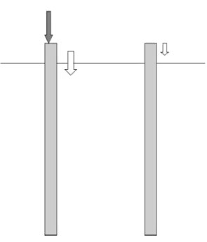
Over the years, behavior of pile foundations have been the subject of deep research. Most studies focused and still focus mainly on pile behavior when subjected to static loading. If one pile of a piled foundation is under static loading, all piles within the deformation field of this pile tend to move in the same direction. Figure 2.2 illustrates an example of two piles where one is subjected to a static vertical force. Due to this load, the pile on the left moves downwards and the pile on the right moves in the same direction. Consequently, in many cases a group of piles will suffer greater displacements than if these were isolated carrying the average load. This means that for groups with high pile density the group efficiency, i.e, the ratio between the total group displacement and the sum of isolated piles displacements if these were loaded separately is smaller than 1. Among many studies of reference, it is important to refer the work of Poulos (1968) and Poulos (1971) where the concept ofinteraction factors presented in Expression 2.1 was introduced and showed that the total group effect can be represented by overlapping the effects of only two piles. However, static pile behavior studies did not provide sufficient information when evaluating dynamic response of pile groups.
αs = additional displacement caused by the nearby pile
displacement of the pile when subjected to it′s own load (2.1)
If the load is dynamic the previous assumption is not always true. When subjected to an harmonic load, both piles will exhibit an harmonic motion. However, the phase of this motion depends on the loading frequency, distance between piles and wave velocity in the soil (H¨olscher, 2014b). Depending on such parameters, the group efficiency may change considerably exhibiting values much higher or smaller than the unity by simply changing the frequency of excitation. This harmonic interaction between two piles is shown in Figure 2.3.
Figure 2.2: Static interaction between two nearby piles, H¨olscher (2014b)
8 Problem Description
and Kausel (1982) uses a numerical solution for the evaluation of the soil flexibility matrix and analytical solutions for the pile stiffness and flexibility matrices. The main disadvan-tage of this and other methods at the time was that these were all of numerical nature and involved discretizing each pile and supporting soil, hence, the application would im-ply substantial computational effort. Given this, Dobry and Gazetas (1988) developed a simple analytical solution to the problem. According to the authors this simple method could be summarized as:
(i) Simple enough to be taught in a course on soil dynamics, and can be well understood and applied by the engineer, even without the help of a computer.
(ii) For a wide range of material parameters, pile separation distances, and frequencies of oscillation, the results of the method are in excellent accordance with rigorous solutions.
(iii) Capable of being applied to all modes of oscillation while retaining its simplicity. (iv) The procedure can be extended to handle pile installation effects in a simplified but
physically sound way.
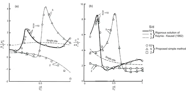
Figure 2.4 compares the simple method developed by Dobry and Gazetas (1988) with the rigorous solution of Kanya and Kausel (1982) for a vertically loaded group of 4 fixed head piles in a homogenous halfspace. These are plotted for different dimensionlesss/dspacings as function of dimensionless frequency(see Equation 2.2) and the dynamic stiffness(a) and damping(b) factors. These factors are defined as the ratio between the dynamic stiffness(KGz) or dashpot(CzG) coefficient and the sum of the static stiffness of the individual single piles(Kzs).
a0 = ω d
cs
(2.2) where,
ω - Angular frequency [rad]
d- Pile diameter [m]
cs - Shear wave velocity of the soil [m/s]
-2
1 0.5
d
ω cs
0.5
d
ω cs 0
0
Figure 2.4: Vertical dynamic stiffness and damping group factors for a group of 2x2 fixed head piles, Dobry and Gazetas (1988)
and frequency the plots exhibit a behavior with the curves for stiffness and damping coef-ficients having pronounced peaks and valleys. It is easily seen that for a small frequency change the dynamic stiffness of the group may considerably change having group factors that lead to safe situations where the dynamic stiffness exceeds by far the unity or po-tential dangerous cases where this considerably decreases to values bellow the well known static group efficiency. For these reasons, dynamically loaded piled foundations require a thoughtful approach, specially for the case of wind turbines working on a dike, since dike safety is of extreme importance in The Netherlands. The main conclusions from Kanya and Kausel (1982) and Dobry and Gazetas (1988) pile-soil-pile interaction studies are:
❼ Behavior of dynamically loaded pile groups is strongly frequency dependent.
❼ Spacing and number of piles have a considerable effect on dynamic stiffness.
❼ Lateral interaction effects are minor when compared with vertical and rocking solic-itations.
10 Problem Description
for pile groups embedded in very stiff soils, typically when the elastic modulus of the soil, Es, is greater than Ep/300, where Ep is the Young’s modulus of the pile. Also, according to the authors, pile groups with high number of piles (typically > 16) the method may slightly overpredict the peaks. With increasing number of piles, the method may become time consuming since the distance between all piles must calculated as well as all interaction factors. In order to face with previous challenges, H¨olscher (2014a) came up with a generalized pile-soil-pile theory, where its solution is derived from the simple method proposed by Dobry and Gazetas (1988). Generalized pile-soil-pile theory uses the same simplifications as the simple method but approaches the problem using a matrix formulation for spacing and dynamic interaction factors, where it allows the calculation of dynamic stiffness for foundations with higher number of piles and many different configurations while keeping its simplicity and low computational effort. Detailed description of the solution is given in section 5.2.
Given the continuous progress on computer technology and the fast increase and avail-ability of computational resources, numerical methods have been attractive tools for the soil-structure interaction problems. Specially the finite element method(FEM) due to its efficiency in dealing with complex geometries and soil heterogeneity. Schoenmaker (2014) approached the problem of a single pile dynamically loaded using to the commercial FEM software PLAXIS and comparing with other numerical and analytical solutions. Overall, results show good agreement with other solutions. However, for high frequencies computer efforts may increase to unfordable calculation times on daily engineering practice.
are calculated using FAST code. A brief explanation of how the software works and the theories involved in the process is made. The wind turbine is briefly described and the natural frequency of the system is calculated. The end of this chapter studies the dynamic wind loads as well as the relevant frequencies of the wind turbine system.
3.2
FAST - Fatigue, Aerodynamics, Structures and
Turbu-lence
FAST its a aero-hydro-servo-elastic code created by National Renewable Energy Labora-tory (NREL) capable of computing the dynamic response of both two and three bladed, conventional horizontal-axis wind turbines. The code was evaluated by Germanischer Lloyd who provided its suitability for the calculation of wind loads for design and certifi-cation of wind turbines (Germanischer Lloyd, 2005).
14 Wind-Turbine Interaction Analysis
but rapidly evolved to the point where is capable of handling flexible systems. FAST considers, for example, the nacelle and hub as rigid bodies and the tower and blades as flexible. Figure 3.1 represents a general multibody system. As shown, the elements of the model are bodies, force elements, joints and a global reference frame. On the surface of the bodies there are parts, called nodes, at which the joints and force elements are attached. The force elements are used to model applied forces and torques. These elements may represent external forces, e.g due to gravity or interaction forces between the bodies, resulting from dampers, springs, actuators or contact. The joints represent any devices that constrain the relative motion of the nodes on the bodies. Joint deformations as a result of the interaction between the system bodies are not considered. Finally, the global reference frame is used to model a known global system motion in the inertial space. The FAST code connects all these bodies with up to 24 degrees of freedom (DOF), which one can turn on or off individually depending on the intended analysis. Some of the considered degrees of freedom by the code are:
❼ Platform translation (surge, sway and heave) and rotation (roll, pitch and yaw).
❼ Tower motion.
❼ Nacelle yaw.
❼ Generator motion.
❼ Blade flexibility, and, tip and flap motion.
Although FAST considers many DOFs, not all of them may be relevant for the required analysis. It is up to the user to understand and define which degrees of freedom to take into account. Figure 3.2 illustrates more specifically some of the available degrees of freedom in the FAST code.
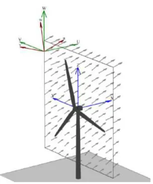
FAST defines a coordinate system depending where and what the input and output pa-rameters are. In order to avoid extensive characterization of this subject, it was chosen to only present the coordinate system relevant for the outputs analyzed in the present thesis. Since the relevant outputs are the actions transmitted from the tower to the foundation, the tower-base coordinate system is chosen as the relevant one. This coordinate system is fixed in the support platform so that it translates and rotates with the platform. Figure 3.3 gives a visualization of the tower-base coordinate system. The origin is at the intersection of the tower axis with the support platform. Thext-axis is the axis pointing at downwind direction (0◦
) whileyt points to the left when looking in the downwind direction. Finally
Figure 3.1: General multibody system and its elements, Schwertassek and Shabana (1999)
16 Wind-Turbine Interaction Analysis
Figure 3.3: Tower base coordinate system considered by FAST (Jonkman and Jr, 2005)
FAST allows the user to model the support platform with a mass-spring-dashpot system, being able to represent an onshore foundation, a fixed bottom offshore foundation or a floating offshore configuration. Not considering any platform type will cause FAST to rigidly attach the tower to the ground through a fixed connection (Jonkman and Jr, 2005). If the user takes platform behavior into account, the software will run a file with mass and inertia parameters of the foundation as well as any considered platform loading. Considering platform loading a user-defined routine is used to compute these effects and returning loads on the platform. This routine contains contributions from any external load acting on the platform other than load transmitted from the wind turbine. For example, these loads should contain contributions from foundation stiffness and damping. Also, the routine assumes that the platform loads are transmitted through a medium like soil (Jonkman and Jr, 2005). Apart from the platform input parameters mentioned before it is necessary to specify damping and stiffness properties in all three translation and rotation components.
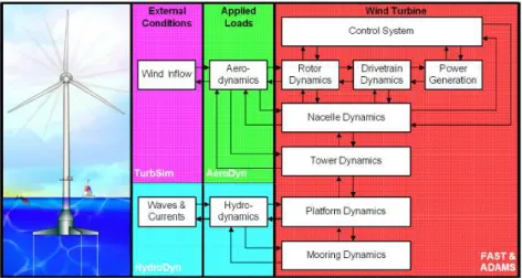
FAST works by interacting with different modules in order to fully achieve time-domain aero-hydro-servo-elastic simulations of wind turbines (see Figure 3.4). Wind flow is created by external programs such as TurbSim and IECWind. FAST with AeroDyn account for the applied aerodynamic and gravitational loads, the behavior of the control systems and the structural dynamics of the wind tower. HydroDyn is a module that computes the applied hydrodynamic loads (Jonkman, 2007). Modeling onshore wind turbines is possible by disabling the hydrodynamic module.
Figure 3.4: FAST code working scheme, Jonkman (2007)
with other software, both need several input data to generate outputs that are a valid input of the following simulator and so on until the requested output by the user is returned by the codes.
3.2.1 Generation of wind field
Wind field is input data for FAST. In order to simulate this wind profiles inx, y and z
directions over time, NREL provides two preprocessors called TurbSim and IECwind that were developed to provide a numerical simulation of wind conditions.
TurbSim is a stochastic, full field, turbulent-wind simulator. It uses a statistical model to numerically simulate time series of wind speed vectors at points in a two-dimensional vertical rectangular grid (Jonkman and Kilcher, 2012). Figure 3.5 gives an example of a typical TurbSim grid as well the coordinate system used by the code. The capital letters point along the inertial reference frame while the others refer to the system aligned with the mean wind. As said before, TurbSim output can be used as input into AeroDyn which later makes the connection with FAST. The code simulates wind flows that contain bursts of turbulence. It generates aleatory components of varying wind speed, wind shear and direction around mean parameters provided by the user. TurbSim allows the creation of many broad spectrum wind scenarios. Also, the software has the possibility of changing the wind model suggested by the IEC 61400-11 norm.
IECwind generates discrete hub-height wind-speed history cases, it allows the user to simulate constant mean flow, direction change (over a certain period of time) and other events recommended by IEC 61400-1. Just like TurbSim, IECwind creates a wind file that
1
18 Wind-Turbine Interaction Analysis
Figure 3.5: Example of a grid and the coordinate system used in TurbSim, Jonkman and Kilcher (2012)
is a valid input in AeroDyn.
3.2.2 AeroDyn
AeroDyn is responsible for transforming wind speeds into loads on the blades caused by wind. It does this by first breaking each blade into a number of segments and continuously gathering information about the turbine geometry, operating condition, blade-element velocity and location, and wind inflow from wind input files. Then, it uses this information to calculate the various forces on each segment, which are used to calculate the distributed forces along the turbine blades. The code obtains wind input data from simple hub-height(IECwind) wind files or full-field(TurbSim) wind files that contain turbulent velocity components at points on a grid that covers an area larger than the rotor disc and tower. Several different aerodynamic models are used in AeroDyn. The user has the option of selecting which of these are most applicable to their simulation needs. The most relevant of these aerodynamic models are the wake models which are the blade element momentum theory (BEM) and the generalized dynamic wake theory(GDW).
the-that the airflow is always in equilibrium. It’s is known the-that this is not completely true and it takes some time for the airfoil to adjust to a changing wake resulting from new inflow or turbine operating conditions. In order to properly model this time lag effect it is recommend that the user primarily chooses the generalized dynamic wake (GDW) model (Moriarty and Hansen, 2005). Although this recommendation is made, AeroDyn switches to the BEM method when the mean wind speed is below 8m/s, due to instability of GDW model at low wind speeds.
The generalized dynamic wake model was originally developed for the helicopter industry and later on adopted to wind turbine aerodynamic calculations. The method assumes that the induced velocities are small compared to the mean wind speed and regard the rotor as an infinite number of slender blades (Moriarty and Hansen, 2005). The consequence of this approach is that the model allows for a more general distribution of pressure across a rotor plane than the BEM theory.
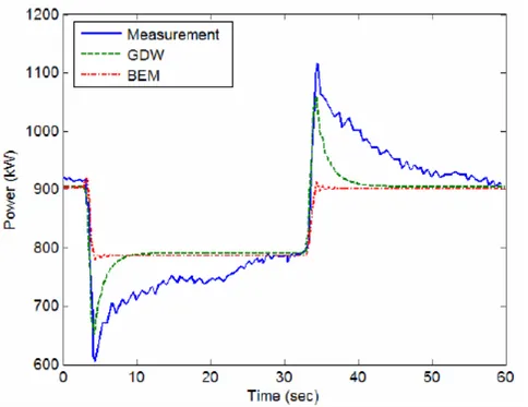
The main advantages of general dynamic wake theory over BEM is that includes inherent modeling of the dynamic wake effect and other phenomena that blade element momentum theory either doesn’t account for or it needs extra corrections in the model. As said before, the dynamic wake effect is the time lag in the induced velocities created by vorticity . Figure 3.6 illustrates an example of this time lag effect on the power production of a wind turbine. More precisely the example shows the measured power output of a wind turbine operating at a 10.6 m/smean wind speed and where the blades are pitched from 0.2◦
to 3.9◦
and then back again to 0.2◦
20 Wind-Turbine Interaction Analysis
Figure 3.6: Generator power output during pitch change, Moriarty and Hansen (2005)
Like the blade element theory, the GDW method has some limitations. The generalized dynamic wake method was developed for lightly loaded rotors and assumes that the in-duced velocities are small relative to the mean flow. This assumption leads to instability of the method at low wind speeds and that is why AeroDyn switches to the blade element momentum theory for speeds smaller than 8m/s.
3.3
Model Parametrization
We are now in conditions to fully define the model for the studied case. Wind action will be defined as well as the wind turbine main parameters. The relevant input parameters are also mentioned in this section.
3.3.1 Wind Turbine Model
Control Variable speed
Blade-Pitch-to-Feather
Blades 3
Rotor orientation Upwind Hub height [m] 90 Rotor diameter [m] 126 Blade length [m] 61,5 Cut-in speed [m/s] 3 Rated speed [m/s] 11,4 Cut-out speed [m/s] 25
Rotational speed range [rpm] 6.9 to 12.1 Tower mass [kg] 347500 Blade mass (each) [kg] 17740 Hub mass (minus the blades) [kg] 56780 Nacelle mass (minus hub and blades) [kg] 240000 Base diameter [m] 6 Base thickness [m] 0,027 Top diameter [m] 3,87 Top thickness [m] 0,019
NREL 5-MW Baseline wind turbine was ”built” gathering available information from manufacturers and from the conceptual models used in the WindPACT2, RECOFF3 and DOWEC 4. It is a conventional upwind horizontal axis wind turbine with three blades and two main control systems, generator-torque controller and rotor collective blade pitch controller. The two control systems are designed to work independently. For the first control the goal is to maximize power capture bellow rated wind speed. When the turbine is working above rated wind speed blade-pitch-to-feather controller is called to regulate the generator speed and also to protect the blades structurally when the wind speed is greater than cut-out wind speed.
2
The land-based Wind Partnerships for Advanced Component Technology.
3
Recommendations for Design of Offshore Wind Turbines.
4
22 Wind-Turbine Interaction Analysis
The tower has a circular hollow steel section with variable diameter and thickness from the base to the top. The base diameter is 6m and 3.8mat the top. The thickness is 0.027m
at the base decreasing to 0.019m at the top. It is also worth mentioning some mechanical properties of the tower material. The elastic modulus was taken to be 210 GP Aand the shear modulus 80.8 GP A. Steel density was increased from the typical value in order to account for paint, bolts and welds that were not accounted for in the tower thickness. Hence, the density was chosen to be 8500kg/m3.
(van der Tempel and Molenaar, 2002) suggest that the structural dynamics of a flexible wind turbine system can be modeled as a beam with a top mass as shown in Figure 3.7. This model was used in order to effectuate a Rayleigh-Ritz modal analysis to calculate the natural frequency of the system. This analysis was made using the engineering tool PTC Mathcad Prime 3.0 and it is presented in appendix A. In order to avoid resonance, the structure should be designed such that its first natural frequency does not coincide with either 1P or 3P intervals. These intervals are rotational frequencies of the rotor, where 1P is given by the rotational speed range shown in table 3.1 and 3P interval is the turbine’s number of blades times 1P frequencies. Results from Rayleigh-Ritz analysis confirm that the natural frequency lies outside these intervals. As seen in Figure 3.8, the tower has a natural frequency of 0.302Hz.
3.3.2 Wind Model
As mentioned in section 3.2.1, a wind profile must first be defined. There are two options, either TurbSim for full-field turbulent wind flows or IECWind for discrete wind profiles. IEC 61400-1 norm requires running a series of design load cases (DLCs) to determine the ultimate and fatigue loads expected over the lifetime of the machine. These design load cases include several wind scenarios and design situations such as normal power pro-duction, occurrence of fault while producing power, emergency shut down, among others. Although this is an important matter to take into account when pursuing certification, this is not the intended case and running all the DLCs would take much more than the available time for this thesis. Also, the goal is to simulate loads on the wind turbine foundation and not other effects on the wind turbine itself. For this reason only one wind scenario and operating condition will be dealt in this thesis.
Figure 3.7: Structural model of a flexible wind turbine system, van der Tempel and Molenaar (2002)
24 Wind-Turbine Interaction Analysis
is defined by a mean value and standard deviation. The norm suggests this turbulence model for several DLCs and (Jonkman, 2007) recommends this model for casual wind turbine evaluation.
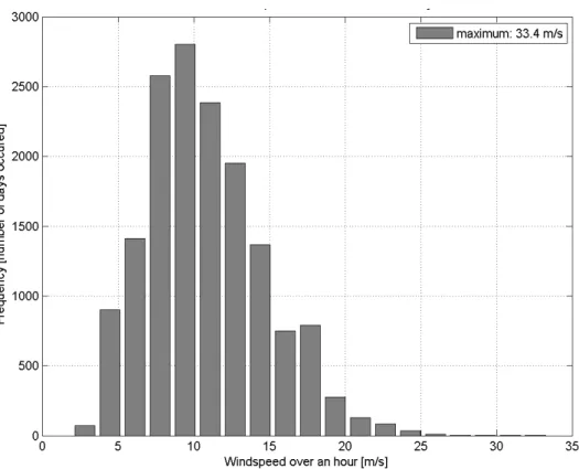
In this thesis, wind data was provided from measurements performed in a weather station close to Lauwersoog, The Netherlands. The provided data can be seen in Figure 3.9 and it represents the hourly wind speed measured over 15552 days. Although this was the only available data , it is important to refer that in terms of wind input data, TurbSim does not need other wind inputs in order to create a reasonable wind spectra.
As Figure 3.9 shows, the most common wind speed observed was around 10m/swhile the maximum verified speed over the period of measurement was 33.4m/s. TurbSim requests a wind speed to serve as mean, and after creates a wind profile that oscillates around this given velocity. This parameter is URef . Although the mean speed given by the data is about 10m/s, dike security is an important matter, and hence, with greater wind speeds, higher loads are expected on the dike. For this reason, URef is set to have the maximum wind speed observed in the whole time of data gathering, i.e,URef is 33.4m/s.
Apart from the mean wind speed considered, TurbSim has several other input parameters. Jonkman (2007) refers that ”‘To generate IEC-type turbulence, many of the parameters in the TurbSim input file can be ignored”’. Given this, Jonkman (2007) gives some guidelines for the parameters that typically do not need to change and those that change every simulation or are dependent on the wind turbine being analyzed. The following parameters should be changed based on the particular wind turbine for which the wind field is being generated:
❼ NumGrid_Z: This parameter controls the number of vertical grid points. It should be large enough to ensure that there is sufficient vertical grid resolution.
❼ NumGrid_Y: This parameter controls the number of lateral grid points. Once again, it should be large enough to ensure that there is sufficient lateral grid resolution.
❼ HubHt: This is the hub height (in meters) of the wind turbine.
❼ GridHeight: Here the grid height is defined. Typically the grid height should be at least 10% larger than the rotor diameter (in meters).
Figure 3.9: Maximum windspeed measured in Lauwersoog weather station over 15552 days
❼ IECtrubc: Defines the turbulence category according to 61400-1 norm.
❼ RefHt: This parameter defines the reference height which is the height (in meters) where the input wind speed is defined. Typically it is the same as HubHt.
Next, the parameters that should be changed for each simulation case:
❼ RandSeed1: This the random seed parameter. Here a number is given which ini-tializes the pseudo-random number generator. The random seed should be changed every simulation in order to create different random wind distributions. When run-ning the same random seed number, the same random phases will be reproduced.
❼ IEC_WindType: Here the wind condition for the turbulent IEC 61400-1 load cases is selected. As mentioned before the chosen wind condition was NTM.
26 Wind-Turbine Interaction Analysis
Since FAST has already the wind turbine model inbuilt some of the parameters are already written on the files provided in the package. Anyhow, the input file was properly filled with the correct values and following Jonkman (2007) guidance it was decided to assume default values for the parameters that would not interfere considerably in the wind simulation. Appendix B.2 contains TurbSim input file ( file extension.inp) with the values used for this specific simulation.
3.3.3 AeroDyn Model
In order to run AeroDyn, at least two other input files are necessary apart from AeroDyn input file it self. One is a wind file (.wnd), which is the output resulting from TurbSim and the other(s) is an airfoil data file (.dat) that is used to properly represent the aerodynamic properties of the problem. The airfoil data is different for every wind turbine and it should be constructed by the user. In this case, the airfoil data is already available and therefore the calculation of drag, lift and pitching moment coefficients (for each angle of attack) was not required.
AeroDyn input file (.ipt) has also some input parameters that do not need to be changed. For this specific case, only the following parameters were altered, leaving the others with their default value:
❼ InfModel: This input controls the dynamic inflow option. The user has two op-tions, eitherDYNIN orEQUIL, which represent generalized dynamic wake model and BEM theory respectively. Given the high wind speeds and the reasons pointed in section 3.2.2,DYNIN is the chosen option for this calculation.
❼ WindFile: Here, the name of the file containing wind data is requested. The input should be something likewindfilename.wnd.
❼ HH: Just like RefHtthis parameter requests the wind turbine hub height.
The full AeroDyn input file can be consulted in appendix B.3.
3.3.4 FAST Model
software. If not, FAST will keep running using the last wind input line. It is also worth mentioning that the time step is separately defined in all three files but it is recommended to be the same in all different codes. So, the integration time step (DT) was defined to be 0.0125 seconds.
Operating condition may change depending on the simulation or design load case in ques-tion. For this, FAST input file includes a turbine control section in order to properly simulate special events. Hereafter, the main control inputs are explained:
❼ PCmode and VSContrl: Both of this parameters are used to turn on or off pitch-control-mode(PCmode) and generator torque for variable speed machines(VSContrl).
❼ BlPitch and B1PitchF: BlPitch controls the initial pitch angle in degrees while
B1PitchF specifies the final pitch angle for pitch maneuvers. These angles must be defined for each blade separately.
❼ TPitManSandTPitManE: These parameters stand for the start (TPitManS) and final (TPitManE) time in seconds for which the pitch override maneuver occurs. Again, these parameters have to be defined for each blade.
❼ TYawManS andTYawManE: This entry parameters refer to the same times as the pre-vious point but for the yaw over ride maneuver.
❼ NacYawF: Here the final yaw angle is defined.
28 Wind-Turbine Interaction Analysis
make sure that the generator is not working i.e not producing power, the generator degree of freedom must be disabled causing the rotor inability to rotate. This means changing
GenDOFto false andRotSpeedassumes a value of 0rpm. Then, all blades must be set to a feathering setting. For this,BlPitchandB1PitchFassume a angle of attack of 90 degrees for all the blades. Also,TPitManSandTPitManEmust be greater than the simulation time. This allows the blades to be in a feathering position the entire simulation and therefore minimizing structural effects due to wind loading. Another thing worth mentioning is that no yaw misalignment is assumed. Hence, nacelle yaw angle (NacYaw) is set to 0 degrees and the yaw DOF(YawDOF) is set to false.
In terms of outputs, forces and bending moments at the base of the tower over time were requested in x, y and z directions. Also, to confirm that no power was produced and therefore the control parameters were set correctly, the rotor speed over time was plotted. Table 3.2 shows the necessary commands to write on OutList to return the desired outputs. Note that the results are printed every 0.05 seconds.
Table 3.2: Requested outputs from FAST
Output Name Description Units
WindVxi Wind speed directed along xt axis m/s
WindVzi Wind speed directed along yt axis m/s
WindVzi Wind speed directed along zt axis m/s
TwrBsFxt Tower base shear force directed alongxtaxis kN
TwrBsFyt Tower base shear force directed alongyt axis kN
TwrBsFzt Tower base axial force (directed alongzt axis) kN
TwrBsMxt Tower base roll moment (about xt axis) kN m
TwrBsMyt Tower base pitching moment (about yt axis) kN m
TwrBsMzt Tower base yaw or torsional moment (aboutzt axis) kN m
LSSTipVxa Rotor angular speed rpm
3.4
Numerical Simulation
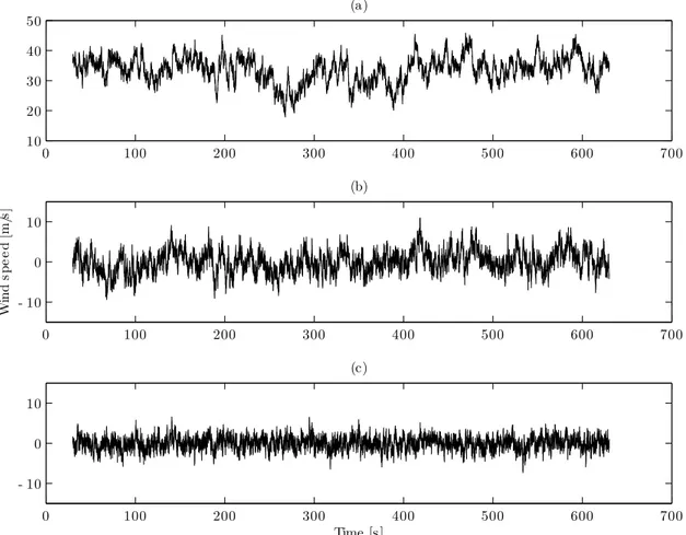
Figure 3.10: Wind speed inxt(a),yt(b) andzt(c) directions
3.4.2 Loads on wind turbine base
30 Wind-Turbine Interaction Analysis
nature of the problem.
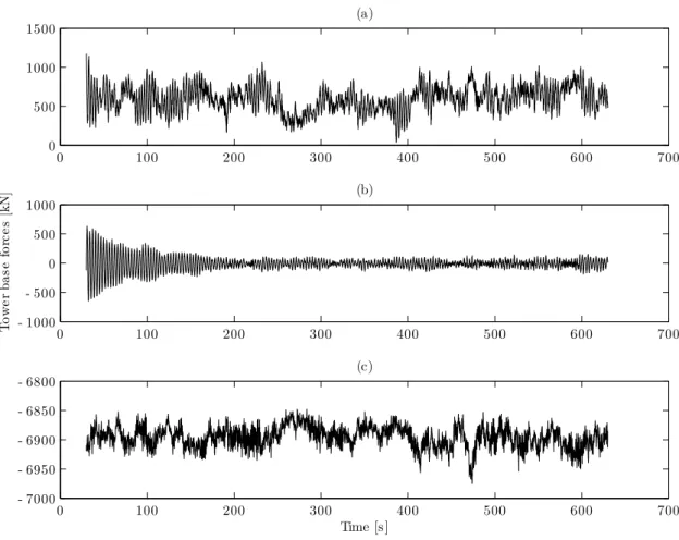
Figure 3.11: Tower base shear forces directed alongxt(a), yt(b) andzt(c) direction
The results for the bending moments can be seen in Figure 3.12. Since the bending moments are function of shear force, the behavior is similar to the one seen in Figures 3.11-a and 3.11-b but now the mean bending moment aroundx axis is clearly greater than zero. Still, the mean bending moment around y axis is much higher than the one registered around x axis. Figure 3.12-c presents the plot for the torsional moment. Giving the low speeds in the transverse direction and the fact that the nacelle is aligned with the wind direction, the torsional moment is small as expected.
Figure 3.13 confirms that no power is being produced during the entire simulation. The figure shows some ”’noise”’ in the plot but when looking to the magnitude of the rotations, one can see that the rotations are very small and oscillate around the mean value of 0
0 100 200 300 400 500 600 700 0
Tower base bending moments [kNm]
0 100 200 300 400 500 600 700
− 1 − 0.5
0 0.5
1x 10 4
Time [s] (c)
Figure 3.12: Tower base moment aroundxt(a),yt(b) andzt(c) axis
0.5
0.4
0.3
0.2
0.1
-0.1
-0.2
-0.3
-0.4
-0.5
0 100
Time [s]
200 300 400 500 600 700
0.0
R
o
to
r
a
n
g
u
la
r
sp
ee
d
[
rp
m
]
32 Wind-Turbine Interaction Analysis
3.5
Discussion
When comparing wind speeds in Figure 3.10, wind speed inxt(a) direction shows greater wind speeds than the ones exhibited in yt(b) and zt(c) directions. While cross-wind and vertical components of wind speed have mean values (at hub-height) close to zero, the wind speed for the nominally downwind component has a mean value of 33.65m/s. Note that this value is extremely close to the input valueUref. It is also important to refer that despiteytandztdirections have almost null mean values (over the simulated period) these present variations during the simulation. Cross-wind speed component varies from -9.41
m/s to 10.99 m/s while vertical wind speed exhibits a variation from -7.35 m/s to 6.57
m/s. Given these relatively important variations , actions in these directions can not be neglected a priori because it may influence turbine behavior over the time of simulation. As mentioned in section 3.3.2, TurbSim generates for the nominally downwind component a profile that oscillates around a mean given wind speed. In this case, the wind speed profile forxtdirection presents a variation of 28 m/swith a minimum value of 17.87m/s
and a maximum of 45.87m/s.
Figure 3.11-a confirms that wind in x direction leads to the higher shear forces that the wind turbine is subjected to. Since a wind turbine problem can be seen as a cantilever beam with a concentrated mass at the hub height and the wind action as a horizontal force, the bending moments are expected to be the conditional loads. That is why the plots for the bending moments show such greatness in their values, specially the tower base pitching moment aroundytaxis seen in Figure 3.12-b, i.e, the bending moment caused by the xt axis shear forces. This rocking motion assumes high importance not just for the wind turbine tower but as well as for the foundation which transmit these forces vertically to the soil underneath.
The plots for yt shear forces seen in Figure 3.11-b and bending moment around xt axis in Figure 3.12-a show different behavior. Here the loads progressively decrease until a stationary state is reached. This is related to start up effects where the wind turbine suffers an initial impact (caused by the first wind input) followed by weak solicitation by the wind inyt direction. Due to low damping the structure takes a while to dissipate the
effects of this initial impact.
fast Fourier transform to the given results by FAST. The results for Figure a and 3.14-b refer to plots in xt and yt directions, where it can be seen that the returned frequency for the highest response is about 0.3017Hz. These plots exhibit similar behavior, which was expected since no major changes between directionsxtand yt can be seen. Also, the natural frequency given by the response spectrum has values very close to the natural frequency of the wind turbine calculated from the Rayleigh-Ritz method in section 3.3.1. On the other hand, the plot forztdirection seen in Figure 3.14-c shows different sensibility
in the frequency domain. Here the frequency that returns the strongest response is situated about 1.088Hz.
Figure 3.15 shows the Fourier spectrum for the wind action in all three directions. As it can be seen, the wind action presents a disperse spectrum with higher amplitude for frequencies below 0.5Hzbeing, as expected,xtdirection the one that produces results with higher magnitude. Also, Figure 3.15 helps explaining the response for the first frequencies seen in Figure 3.14-a and 3.14-c, being these due to the wind excitation.
3.6
Conclusions
In this chapter the wind-turbine problem was successfully handled. Introductory concepts about FAST and all the codes related to the software were given as well as the theories behind. This is a multidisciplinary subject and requires a vast knowledge of different areas to fully understand and define all phenomena that take place on a turbine loaded by wind. After plotting the loads caused by the high wind problem in all threex,yandzdirections, the following conclusions were drawn:
34 Wind-Turbine Interaction Analysis
Amplitude
Frequency [Hz] 6 x10
x:0.3017
x:1.088 5
x105
x104 4
2
0
6
4
2
0
6
4
2
0 0
0
0
0.5 1 1.5 2 2.5 3 4
(a)
(b)
(c)
3.5 4.5 5
0.5 1 1.5 2 2.5 3 3.5 4 4.5 5
0.5 1 1.5 2 2.5 3 3.5 4 4.5 5
Figure 3.14: Amplitude spectrum of the wind turbine’s response calculated using fast Fourier transforms inxt(a),yt(b) andzt(c) directions
0 0.5 1 1.5 2 2.5 3 3.5 4 4.5 5
0 1 2 3
4 (a)
0 0.5 1 1.5 2 2.5 3 3.5 4 4.5 5
0 0.5
1 (b)
Amplitude
0 0.5 1 1.5 2 2.5 3 3.5 4 4.5 5
0 0.1 0.2 0.3
0.4 (c)
Frequency [Hz]
Figure 3.15: Amplitude spectrum of the wind action calculated using fast Fourier transforms in
relevant role. This is expected when the wind turbine is properly working (even if the rotor is not producing power). Nevertheless, it is important to refer that fault conditions might create conditions for yaw misalignment and therefore increasing torsional solicitation of the wind turbine.
❼ Plots for the horizontal xt force and pitching moment confirm that the highest so-licitation is due to wind action directed along xt axis.
❼ Finally, response frequency analysis show that the frequencies that return higher response are close to 1 Hzand below.
After building a wind interaction model that allowed the computation of the dynamic wind loads acting at the foundation of the wind turbine, it is necessary to define and evaluate all the parameters of the geotechnical model. Figure 4.1 represents schematically the model in question. As said, the wind turbine foundation is implemented on the top of a dike which it’s materials and also the foundation are yet not defined. All these variables are defined using a case-study site which is developed in this Chapter.
First the evaluation of the soil is made using CPT data from three soil tests carried out on the dike. Afterwards, load definition is made using results from Chapter 3 and finally a foundation preliminary design is performed. After this chapter all conditions will be met towards a pile-soil-pile interaction analysis.
4.2
Soil Characterization
4.2.1 Field Data
38 Geotechnical and Foundation Model
CPT Head
Dike’s material
Naturally deposited soils
Figure 4.1: Schematic profile of the geotechnical model being defined
location where thein-situtests were made and their corresponding names. The coordinates for each CPT can be seen in table 4.1. As for the data, this is of public domain and made available by DINOloket . DINOloket is a public access website that gathers information of geotechnical testing performed in The Netherlands territory. For the present thesis, all the chosen soil parameters are derived from the CPT data available on DINOloket, more specifically by 3 tests: S02G00190, S02G00208 and S02G00206.
Table 4.1: Cone penetration tests coordinates
CPT name Coordinates S02G00190 5324’28.52”N 6 9’18.08”E S02G00208 5324’32.37”N 6 9’31.13”E S02G00206 5324’35.59”N 6 9’42.05”E From CPT data the gross given parameters are:
❼ The beginning elevation or the head (m)
❼ Depth (m)
❼ Cone resistance,qc (M P a)
Figure 4.2: Local of CPT testing, taken from Google Earth version 7.1.2.2041
❼ Friction Ratio, Rf (%)
From these measurements and through several correlations, a CPT test offers soil profiling, material identification and evaluation of geotechnical parameters. CPT is a soil test with extensive applications in a wide range of soils. Although the CPT is limited primarily to softer soils, with modern large pushing equipment and more robust cones, the CPT can be performed in a stiff to very stiff soils (Robertson and Cabal, 2012). It should be noted that an ideal soil characterization should have different types of in-situ soil testing and also samples to perform laboratory tests.
Figure 4.3 presents the measured gross parameters over depth returned by CPT S02G00190. In section 4.2.2 CPT interpretation is made in order to define the required soil parameters for the intended analysis. For the present thesis, these are shear strength, state and elastic parameters. However, different types of analysis and constitutive models may change the required parameters that are necessary to estimate.
4.2.2 Data interpretation
40 Geotechnical and Foundation Model
Figure 4.3: Measured field data from CPT S02G00190
One of the major applications (and advantages) of the CPT test is for soil profiling and defining soil type. Typically, at first sight one can identify different soil mechanical behav-ior by analyzing the cone resistance and the friction ratio. When qc has a high value and Rf returns a low one, it means that a sandy-type behavior is expected. The contrary is verified when dealing with soft soils. Figure 4.3 illustrates exactly this. In the beginning higher cone resistance values and small friction ratio are observed, which give a sandy soil expectation. With increasing depth and specially after -2 m elevation a change in these parameters can be seen. Rf increases while qc starts decreasing. This is clearly a layer transition and a cohesive soil is expected. The same line of thought can be made for the other CPTs.
The best way to calculate the total unit weight of a soil is by obtaining an undisturbed sample and weighting a known soil volume. When such procedure is not possible, rela-tionship 4.1 (Robertson, 2010) can be used to estimate the total unit weight from CPT results:
γ
γw = 0.27 [logRf] +
log qt
pa
friction with depth due to the increase in effective overburden stress, a new normalized SBT chart was suggested by Robertson (1990). This new chart requires normalization of these parameters. The normalized soil behavior type(SBTN) chart shown in Figure 4.4 apart from identifying results for most young, un-cemented, insensitive normally consolidated soils also identifies ground response, such as increasing soil density, over consolidation ratio, age and soil sensitivity. The soil type corresponding to the numbers seen in Figure 4.4 can be consulted in table 4.2. Nevertheless, it should be reminded that these charts are meant to provide guidelines to the soil behavior type.
To simplify the application of the normalized soil behavior type chart shown in Figure 4.4, the normalized parameters can be combined into one soil behavior type index(Ic), where Ic is the radius of the essentially concentric circles that represent the boundaries between each SBT zone (Robertson and Cabal, 2012). Ic is defined as:
Ic =
q
(3.47−logQt)2+ (logFr+ 1.22)2 (4.2) where, the normalized cone penetration resistance (Qt) is expressed in a non-dimensional
form and taking into account thein-situ vertical stresses:
Qt= qt−σvo
σ′ vo
(4.3)
The normalized friction ratio(Fr) can be expressed as:
Fr= fs
qt−σvo
42 Geotechnical and Foundation Model
Figure 4.4: Normalized CPT soil behavior type chart, Robertson (2010)
in table 4.2. Note that this index does not apply to zones 1,8 and 9 shown in Figure 4.4. Profiles ofIc provide extra help to identify the continuous variation of soil behavior based
on CPT results. Figure 4.5 illustrates for CPT S02G00190 a profile using a color code developed to aid the visual representation of SBT on a CPT profile. This method was also used on the layer definition process.
Table 4.2: Soil behavior type index boundaries, Robertson and Cabal (2012)
Zone Soil Behavior Type Ic
1 Sensitive, fine grained N/A
2 Organic soils clay >3.60 3 Clays silty clay to clay 2.95−3.60 4 Silt mixtures clayey silt to silty clay 2.60−2.95 5 Sand mixtures silty sand to sandy silt 2.05−2.60 6 Sands clean sand to silty sand 1.31−2.05 7 Gravelly sand to dense sand <1.31 8 Very stiff sand to clayey sand N/A
9 Very stiff, fine grained N/A
As seen in Figure 4.5, the soil profile suggests that granular and cohesive soil may be found with depth. It is then important to estimate both friction angle and undrained shear strength parameters depending on the type of soil. Also, these parameters might indicate what kind of soil we are dealing with. Soils that exhibit a drained behavior have particularly high friction angles(φ′
) while undrained like soils have low φ′
SBTn legend
1. Organic material - clay
2. Clay to silty clay
3. Clayey silt to silty clay clay
4. Silty sand to sandy silt
5. Clean sand to silty sand
6. Gravely sand to dense sand
Figure 4.5: Soil behaviour type index ploted over elevation for CPT S02G00190
For the friction angle, two correlations are used. This allows to have a greater number of results and to evaluate if different correlations give alike results. The first relation presents the Robertson and Campanella (1983) correlation and latter Kulhawy and Mayne (1990) relationship:
tanφ′
= 1 2.68
log
qc σ′
vo
+ 0.29
(4.5)
φ′
= 17.6 + 11×log (Qt) (4.6)
For undrained shear strength the correlation most commonly suggested in bibliography is from Lunne and Eide (1976):
su= qt−σvo
Nkt (4.7)
44 Geotechnical and Foundation Model
to 18 and tends to increase with increasing plasticity and decrease with increasing soil sensitivity. Undisturbed soil samples must be obtained in order to properly define Nkt
but when such resources are not available Bowles (1998) suggests a value of 14 to be satisfactory to use in Equation 4.7.
The last estimated soil parameter is Young’s modulus(E). This modulus has been defined as that mobilized at about 0.1% strain. This is referred by (Robertson and Cabal, 2012) to be highly to moderately applicable to foundation design. The young modulus is then defined as:
E =αE[qt−σvo] (4.8) where,
αE = 0.015
h
10(0.55Ic+1.68)
i
(4.9) Correlations for estimation of angle of friction, undrained shear strength and elastic mod-ulus were presented in this section. However, as referred by (Bowles, 1998), a user should use them cautiously and these correlations should be plotted into charts. As the trend for each parameter develops, equation results may be revised.
4.2.3 Layer definition and obtained results
CPT results refer purely and only to the volume of soil tested and not for all the area of implementation. For this reason it is important to treat results all together and separate what might be reasonable results from singularities and isolated characteristics of a single CPT profile. The true soil characteristics should lay somewhere in between all results and the more tests, greater the degree of confidence in the estimations made. For this matter and to avoid extensive result presentation, the results shown in this section are charts containing all the data together.
As mentioned in the previous section, when looking at readings of cone resistance and friction ratio together it is possible to start defining the type of soil that the CPT is pen-etrating. When this trends tend to change with depth a layer change can be anticipated. This is what can be seen in Figure 4.6. The figure showsqc(a) andRf(b) plotted over
suggesting the other way.
In the interest of making a better evaluation of the dike materials, a chart with the continuous soil behavior type index was elaborated. This plot shown in Figure 4.7 returns
SBTN index using a standard color code which is very helpful on the soil definition.
According to (Robertson and Cabal, 2012) independent studies have shown thatSBTN
charts typically have greater than 80% reliability when compared with soil samples. For this reason and that no samples were available, special attention should be made to the results returned by this method when defining the layer materials.
46 Geotechnical and Foundation Model
Figure 4.6: Cone resistance (a) and Friction ratio (b) CPT results
SBTn legend
1. Organic material - clay 2. Clay to silty clay
3. Clayey silt to silty clay clay
4. Silty sand to sandy silt
5. Clean sand to silty sand 6. Gravely sand to dense sand
the third layer, difference is found when comparing results for S02G00206 and S02G00208 with S02G00190. Here the plot for the first pair suggests a higher value for γ than for S02G00190 CPT. Once again, when deliberating this parameter one should have attention to this outcome and chose a value that is capable of representing all results.
Chart 4.9 shows correlation results for the friction angle. These display similar tendency to the ones observed in Figure 4.8 forγ estimation. For the case of φ′
on the third layer, returned values have a difference between S02G00190 and the other two of about 10◦
. Anyway, it is clear that when CPT S02G00190 reaches a certain depth this parameter rapidly increases, which leaves the impression that this layer has good conditions to found the piles tips if necessary.
As for the undrained shear strength, the results shown in Figure 4.10 appear to be relatively close together if we ignore the registered peaks in the beginning and end of the layer. Most points locate between 150 and 300kP a leaving a reasonable confidence when attributing ansu value to the layer.
Finally elastic modulus charts are presented in Figure 4.11. Also here the results show the same peaked tendency as the first layer plots forγandφ′
and significant difference on third layer. When dealing with this results variation, caution is advised and some conservatism may be taken when choosing this parameters. On the contrary plots for the second layer present points close together with minimal deviations which enhance the confidence for the young modulus on the second layer.
4.2.4 Adopted Soil Parameters
48 Geotechnical and Foundation Model
Figure 4.9: Plotted results for the angle of friction on first and third soil layer
50 Geotechnical and Foundation Model
parameters that define mechanically each layer. The soil is modeled as having three layers with first being related to the dike’s material. Both the first and third layers are characterized as having their shear strength defined purely by an angle of friction while the second layer is described as behaving like an undrained type of soil and therefore having it’s shear strength characterized by just the undrained shear strength. In terms of elevation, the three CPTs executed do not start at same height, so the surface quota was defined as the average of all CPTs head elevation with a value of 8.7m. The second layer is 4 meter thick and it starts at around -2mheight. The last layer starts at -6 meters and the longest CPT ends at about -10m not having information after this depth.
In the interest of choosing soil parameters it was taken a moderately conservative posture, meaning that since CPT is our only test and all parameters are based on correlations, it is prudent to take into account the variability of the results and proceed to a safe choice of the mechanical parameters. Table 4.3 shows the chosen values for all the mechanical parameters. These values were chosen based on the plots presented in the previous section. It should be noted that each person may have a different view over parameter choice depending on the experience, geotechnical application and available data.
52 Geotechnical and Foundation Model
Table 4.3: Estimated soil parameters
Layer φ′
[◦
] su [kP a] γt [kN/m3] E [M P a] ν
1 39 - 20 90 0,35 2 - 200 18 65 0,4 3 33 - 19 100 0,35
Regarding Poisson’s ratio, since no other information was available, values suggested by bibliography were adopted, more precisely values proposed by (Bowles, 1998). Here the author suggests a value range of 0.3 to 0.4 for sands and for undrained type of soils from 0.3(silty soils) to 0.5(saturated clay soils). Since no information was given, it was chosen the average value as being the representative for each layer.
4.3
Foundation Preliminary Design
As mentioned before, the foundation being analyzed is a foundation composed by a group of piles. Piles are structural members that are used to transmit surface loads to lower levels in the soil mass. This transfer may be mainly vertical distribution of the load along the pile shaft by means of friction (floating pile) or direct load application to the pile tip (end-bearing pile). Nonetheless, all piles support loads as a combination of shaft resistance and tip resistance. The quality of a deep foundation depends on the construction technique, equipment among other factors. Such parameters are not easy to quantify or take into account in normal design procedures. For this reason the Canadian Geotechnical Society refers that it is desirable to design deep foundations on a loading test basis of actual foundation units, also, monitor construction to ensure that design requirements are fulfilled. However, it is easily understandable that most projects may not have this kind of resources available.
In this section a preliminary design of a piled group foundation is made using well-known analytical solutions derived from plasticity theory and using Eurocode 7 in order to meet safety requirements.
4.3.1 Adopted foundation Loads