Radial basis functions collocation method for solution of MagnetohydrodynamicNono boundary-layer flows

http://www.bipublication.com

Research Article

Radial basis functions collocation method for solution of

MagnetohydrodynamicNono boundary-layer flows

1

Masomeh Aghamohamadi and 2Jalil Rashidinia

1_{Department of Mathmatics,College of basic science,}

Karaj Branch,Islamic azad University, Alborz,Iran,P.O.Box 31485-313 Email: ma.aqamohamadi@kaiu.ac.ir

2

School of Mathematics, Iran University of Science and Technology, Narmak, Tehran 1684613114, Iran

Email: rashidinia@iust.ac.ir ABSTRACT

In this paper, axisymmetric flows over stretching surfaces in a porous medium in the presence of a magnetic field with the navier boundary condition have been considered. The governing partial differential equation (PDE) has been reduced to nonlinear ordinary differential equation (ODE) by using suitable similarity transformations. The collocation methods based on Multiquadric (MQ) Radial basis function (RBF) has been developed for the arising ODE. The method has been tested on an example to show that the presented method is easy applicable and simple. The computed solution is in a good of the solved example with the exact solution. This has been verified by the plotted graphs.

Keywords: Collocation; MQ; Nano boundary-layer flows; Radial basis function; method. INTRODUCTION

The notion of a boundary layer was first introduced by (Prandtl,1904) to explain the discrepancies between the theory of inviscid fluid flow and experiment. In the classical boundary-layer theory, the condition of no-slip near the solid walls is usually applied, where the fluid velocity component is assumed to be zero relatihve to the solid boundary that is not true for fluid flows at the micro-and Nano scale. (Gad-el-Hak. M, 1999) showed that the no-slip condition is no longer valid instead, a certain degree of tangential slip must be allowed. The Nano boundary-layer fluid flows mean Nano scale flows which have many applications in micro-electro-mechanical systems. In recent years, because of importance of applications of fluid flow over a stretching sheet in industry, such as polymer processing of a chemical engineering plant and metallurgy, some interests have been given and some useful

boundary-layer flows with Navier boundary condition. Existence and uniqueness solutions were established by (Akyildiz. F. T and et al ,2011) . They considered the three dimensional nano boundary-layer viscous flows over a horizontal axisymmetric two-dimensional stretching surface.Let be the velocity components along (x,y,z) axes, respectively. The three dimensional nano boundary-layer flows of an incompressible fluid with constant electrical conductivity over a horizonal axisymmetric two dimensional stretching elastic sheet through the porous media is as follows:

(1)

, (2)

(3)

(4)

with the boundary conditions:

(5)

Where are the fluid density, pressure, uniform transverse magnetic field of strength, electrical conductivity, viscosity and permeability of the porous medium and is stretching constant and is a parameter that describes the type of plate stretching respectively. We have two-dimensional stretching wall if m 1, and for

2

m  _{we have}

axisymmetric stretching. is the constant of suction/injection velocity at the wall. when injection occurs from the surface and velocity is due to suction velocity.The induced magnetic field is assumed negligible. Also external electric field is zero because of polarization of charges. According to (Wu. L. A 's article, 2008) slip velocity at the wall, can be presented as:

(6)

Where is the momentum

accommodation and .

The positive parameter is the dimensionless slip parameter. First of all we introduce the dimensionless function with similarity variable as follow:

(7)

Where is the kinematic viscosity. By using Equation 7 with Equations 2-4 we can get a non-dimensional nonlinear ordinary differential equation governing the resulting boundary-layer flow, the Navier–Stokes equation as follows:

(8)

With the following boundary conditions:

(9)

Where and ,are the magnetic

and dimensionless permeability

parameters. and <0 denote the

first order velocity slip parameter and the second order velocity slip parameter (see (VanGorder. R. A, 2010) for more details). We denote that . The solution

of the Navier stock equation (8) with boundary conditions (9 ) has been considered by many authors. (Samadpoor. S et al ,2013) investigated the model numerically and obtained the solution of the problem. In recent years

numerous models in boundary layers flow, such as Hankel-pade method by (Abbasbandy and et al, 2009, 2012, 2013) and (Roohani Ghahsareha and et al, 2014), Homotopy analysis method by (Mousa M. M, Kaltayev. A, 2010), (Rashidi. M. M and Gangi. D. D, 2010), (Yao. B, 2009), Adomian decomposition methods by (Alizadeh. E and et al,2014), (Ghehsareh. HR and et al, 2012), (Raftari. B and et al, 2012), (Samadpoor and et al, 2013), spectral methods by (Babolian. E, Hosseini. M. M, 2003, 2012) , (Darvishi and et al , 2008) and (Ghovatmand. M and et al, 2011), (Hany N. Hassan, Hassank. Sale, 2013) and (Hosseini. M., M, 2005) and others (Abbasbandy and et al, 2010,2012), (Aly. E. H and Hassan. M. A, 2014) and (Lihua Guo and et al,2014). In this work, our interesting is to compute the similar solution of Equation (8) with boundary conditions (9).

This paper is organized in six sections. In section two, summery of RBFs in general have been given and in section three a mesh free method based on the RBFs has been applied to Equation (8) subject to its boundary conditions (9).

In section four, numerical results and discussions are brought and finally in section five and six, there are conclusion and references.

RBF Introduction

The method of RBF is a well-known family of meshless methods that is the center point is not necessarily structured.

These functions have been used for solving various kind of problems such as (Abbasbandy. S and et al, 2012-2014), (Buhmann. M and Dyn. N, 1993), (Brown. D. and et al, 2005), (chantasiriwan. S, 2004), (Micchelli. CA,1986) and (Sarra. SA, 2005). In all the interpolation methods for scattered data sets, RBFs outperforms all the other

methods regarding accuracy, stability, efficiency, memory requirement and simplicity

of the , where

is the Euclidian norm.

The RBF may also have a shape parameter c, in which case is replaced by .Some of the most popular RBFs are given in Table.1.

Table.1:Some of the most popular radial basis functions..

The RBF interpolant is a linear combination of RBFs centered at the scattered points :

(10)

When we use infinitely smooth RBFs, the approximations feature spectral convergence as the points get denser. This has been proven strictly only for some special cases,like ( Buhman. M and Dyn. N 's article , 1993). We will see that the accuracy of the solution is a function of the shape parameter and that very small values of c often give the best results. The shape parameter affects both the accuracy of the approximation and the conditioning of the interpolation matrix (Sarra. SA, 2005).According to definition of approximation of can be rewritten as follow respectively:

, (11)

(12)

The expansion coefficients can therefore be obtained by solving the linear system ,

where

= ,

And .

Becauseof then

, consequently the matrix $A$

is symmetric. On the other hand according to investigations of (Schoenberg. IJ, 1938), (Sarra. SA, 2005) and (Micchelli. CA, 1986), $A$ is nonsingular i.e, it has an unique interpolates of the form Equation 2.11 and no matter how the distinct data points are scattered in any number of space dimensions.

A mesh free method based on RBFs:

For solving the Equation (8) with the boundary conditions (9) , the mesh free method based on the RBF is considered. It is supposed that the closed form approximating function Equation (11) obtained from a set of training points and its derivative of any order, that is:

, (13)

Where p is the order of approximation derivative. By using Equation13 in Equation with the boundary conditions 9, we obtain the following equations:

(14)

Where and and F

is known function and are known constants. By substituting Equation 11 in 14 and using 13 we have:

To obtain the coefficient , we define the residual function:

(15)

, then equalize Equation 15 to zero at N-p interpolate node with p boundary conditions, i.e:

(1

6)

Now we can approximation by above explanation as:

. Here have defined as:

To solve the problem:

By equalizing to zero at N-3 interpolate nodes .

RESULT AND DISCUSSION

In this section the presented technique is employed to approximate the similarity solutions of the Equation 8 with given boundary conditions 9 in both cases, m=1,the viscous flows over a two dimensional stretching surface, and m=2, the viscous flows over an axisymmetric stretching surface. The computed solutions of the similar stream function, , velocity distribution of flow, and the function of shear stress, , for the case of the viscous flows over a two dimensional stretching surface, m=1 and by sitting

0.5, 2, 1, 1

p

k  s 



 



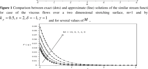
 and for several

Figure 1 Comparison between exact (dots) and approximate (line) solutions of the similar stream function,

for case of the viscous flows over a two dimensional stretching surface, m=1 and by letting

0.5, 2, 1, 1

p

k  s 



 





and for several values ofM .

Figure2Comparison between exact (dots) and approximate (line) solutions of the velocity distribution of flow for case of the viscous flows over a two dimensional stretching surface, m=1 and by letting

0.5, 2, 1, 1

p

k  s



 



 and for several values ofM .

Figure 3Comparison between exact (dots) and approximate (line) solutions of the function of shear stress, for case of the viscous flows over a two dimensional stretching surface, m=1 and by letting

0.5, 2, 1, 1

p

k  s 



 



 and for several values ofM .

Figure 4Comparison between exact (dots) and approximate (line) solutions of the similar stream function for case of the viscous flows over a two dimensional stretching surface, m=1 and by letting

5, 2, 1, 1

Figure 5Comparison between exact (dots) and approximate (line) solutions of the velocity distribution of

flow, for case of the viscous flows over a two dimensional stretching surface, m=1 and by letting

5, 2, 1, 1

M  s



 



 and for several values ofk_p.

Figure 6Comparison between exact (dots) and approximate (line) solutions of the function of shear stress, for case of the viscous flows over a two dimensional stretching surface, m=1 and by letting

5, 2, 1, 1

M  s       and for several values ofk_p.

In Figures 4-6 the approximated results for

,

and

for case of the viscous

flows

over

a

two

dimensional

stretching

surface,

m=1

and

by

choosing

and for various values of

k_p

are plotted and

compared with the exact solutions.

Figure 7. Comparison between exact (dots) and approximate (line) solutions of the velocity distribution of flow,f ( )



for case of the viscous flows over a two dimensional stretching surface, m=1 and by letting

5, _p 0.5, 1, 1

Figure 8. Comparison between exact (dots) and approximate (line) solutions of the function of shear stress, for case of the viscous flows over a two dimensional stretching surface, m=1 and by letting M 5,k_p 0.5,



 1,



1 and for several values ofs .

Also in figures 7-8, obtained results for

and

for m=1 and by choosing

5, _p 0.5, 1, 1

M  k 



 





and for several values of s are plotted and compared with the

exact solutions. From these presented results, it is clearly concluded that the approximated

solutions computed from the RBF collocation method are in excellent agreement with the

exact solutions.

Also the radial basis functions collocation method is applied for solving the governing

problem for case of the viscous flows over an axisymmetric stretching surface, m=2. In this

case, we clearly show the effect of different values of

on

,

and

. The numerical results are obtained for the region

.

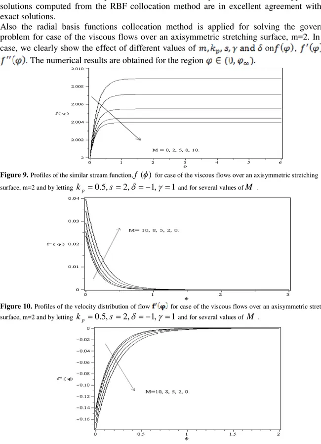
Figure 9. Profiles of the similar stream function,f ( )



for case of the viscous flows over an axisymmetric stretching surface, m=2 and by letting k_p 0.5,s 2,



 1,



1 and for several values ofM .

Figure 11. Profiles of the variation of the shear stress for case of the viscous flows over an axisymmetric stretching surface, m=2 and by letting k_p 0.5,s 2,



 1,



1 and for several values ofM .

Figure 12. Profiles of the similar stream function (left ), velocity distributions (center) and variation of the shear stress, , (right) for case of the viscous flows over an axisymmetric stretching surface, m=2 and by letting M 5,s2,



1,



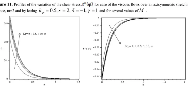
1 and for several values of k_p.

Figures 9-11 depict effect of M on , and . From Figure 9 can be understood that by decreasing value of investigated parameter M, increases, as it is shown in Figure 11. Whenever M decreases, decreases too. These results are similar to Figures 1-3, when m=1. According to Figure 12 whenever k_pincreases, increases too, but decreases. The thickness layer

decreases with decreasingk_p.

Figure 13. Profiles of the velocity distributions (left) and variation of the shear stress (right) for case of the viscous flows over an axisymmetric stretching surface, m=2 and by letting

5, _p 0.5, 1, 1

M  k 



 



 and for several values of s.

Figure15. Profiles of the similar stream function (left ), velocity distributions (center) and variation of the shear stress, (right) for case of the viscous flows over an axisymmetric stretching surface, m=2 and by letting M5,s2,



1,kp1 and for several values of



.

For all plots, it can be understood that , as a function of is negative for all values of all parameters, . Comparing Figures 7-8 and 13 can be deduced that decreasing |s|, increasing while s has a direct effect on , i.e fluid flow at nano scales and at the wall decrease with a decreasing in |s|. According to profile of Figure 14, effect on , inversely while decreasing rapidly. In Figure 15 the effect of



on the , and is shown when M5,s2,



1,kp1when m=2. When



decreases the thickness layout and velocity distribution of flow increased considerably, while decreases, same as before.

CONCLUSION

In this study the IMQ RBF collocation method is employed for the solution of boundary-layer problems is presented. The numerical solutions are given for different values of model's parameters. The effects of parameters on the Nano boundary thickness is investigated and at the end treatment of similar stream function, velocity distribution and shear stress are plotted by variable parameters The figures show that the computed solutions are in good agreements with the exact solutions.

REFERENCES

1. Abbasbandy.S, Hayat. T. (2009). Solution of the MHD Falkner–Skan flow by Hankel–Pade method. Phys. Lett. A . 373 : 731-734.

2. Abbasbandy. S, Hayat. T, Ghehsareh. H R, Alsaedi. A. ( 2010). MHD Falkner-Skan flow of Maxwell fluid by rational Chebyshev collocation method. Applied Mathematics and Mechanics. 34 ,8 : 921-930.

3. Abbasbandy. S, Roohani Ghehsareh.( 2012). H. Solutions of the MHD flow over a non-linear stretching sheet and nano boundary layers over stretching surfaces, Internat. J. Numer. Methods Fluids. 70,10 :1324-1340.

4. Abbasbandy. S, Roohani Ghehsareh.H, (2013). Solutions for MHD viscous flow due to a shrinking sheet by Hankel-Pade method, nternat. J. Numer. Methods Heat Fluid Flow. 23,2: 388-400.

5. Abbasbandy. S, Roohani Ghehsareh.H, Hashim.I. (2012). An accurate solution for the steady flow of third-grade fluid in a porous half space, Walailak J. Sci. \& Tech. 9, 2: 153-163.

6. Abbasbandy. S, Ghehsareh. H.R, Hashim. I. (2012). An approximate solution of the MHD flow over a non-linear stretching sheet by rational chebyshev collocation method. Sci. Bull. A. 74 , 47e58.

for a non-classical 2-D diffusion model, Engineering Analysis with Boundary Elements.39. 121-128.

8. Abbasbandy. S, Roohani Ghehsareh. H, Hashim. I. (2013). A meshfree method for the solution of two-dimensional cubic nonlinear Schrodinger equation, Eng. Anal. Bound. Elem. 37. 6. 885-898. 9. Abbasbandy. S, Roohani Ghehsareh. H ,

Hashim. I, Alsaedi. A. (2014). A comparison study of meshfree techniques for solving the two-dimensional linear hyperbolic telegraph equation, Engineering Analysis with Boundary Elements. 47. 10–20 .

10. Abbasbandy. S, Roohani Ghehsareh. H,Hashim. I. (2012). Numerical analysis of a mathematical model for capillary formation in tumor angiogenesis using a meshfree method based on the radial basis function, Eng. Anal. Bound. Elem. 36. 1811-1818.

11. Akyildiz. F.T, Bellout .H, Vajravelu. K, Van Gorder. R.A. (2011). Existence results for third order nonlinear boundary value problems arising in nano boundary layer fluid flows over stretching surfaces, Nonl. Anal: Real World Appl. 12. 2919–2930. 12. Alizadeh. E, Farhadi. M, Sedighi. K,

Ebrahimi-Kebria. H. R, and Ghafourian. (2014). A Solution of the Falkner-Skan equation for wedge by Adomian Decomposition Method, Communications in Nonlinear Science and Numerical Simulation .14 3. 724–733.

13. Aly. E.H, Ebaid. A, (2012). on the exact analytical and numerical solutions of Nano boundary-layer fluid flows, Abst. Appl . Anal.

2012. 22.

http://dx.doi.org/10.1155/2012/415431. (Article ID 415431).

14. Aly. E.H, Hassan. M.A. (2014). Suction and injection analysis of MHD nano boundary-layer over a stretching surface through a porous medium with partial slip boundary condition, J. Comput. Theor. Nanosci. 11. 827–839.

15. Aly. E.H, Vajravelu. K. (2014). Exact and numerical solutions of MHD nano boundary-layer flows over stretching surfaces in a porous medium, Applied Mathematics and Computation. 232 191– 20.

16. Babolian. E, Hosseini. M. M. (2012). A modified spectral method for numerical solution of ordinary differential equations with non-analytic solution, Applied Mathematics and Computations . 132 , 2-3. 341-351.

17. Babolian. E, Hosseini. M. M. (2003). Reducing index and spectral methods for differential-algebraic equations, Applied Mathematics and Computations .140. 77-90.

18. Brown. D, Ling .L, Kansa .EJ, Levesley . J. (2005). On approximate cardinal precondition- ing methods for solving PDEs with radial basis functions. Eng Anal Boundary Elem, 29: 343–53.

19. Buhmann. M and Dyn. N. (1993). Spectral convergence of multiquadric interpolation, Proc. Edinburgh Math. Soc. 36. 2. 319-333.

20. Chantasiriwan. S. (2004). Cartesian grid method using radial basis functions for solving Poisson, Helmholtz, and diffusion– convection equations. Eng Anal Boundary Elem . 28. 1417–1425.

21. Darvishi. MT, Kheybari. S, Khani. F. (2008). Spectral collocation method and Darvishi’s preconditionings to solve the generalized Burgers–Huxley equation, Communications in Nonlinear Science and Numerical Simulation. 13 ,10. 2091-2103. 22. Gad-el-Hak. M. (1999). The fluid

mechanics of macrodevices-the Freeman scholar lecture, Journal of Fluids Engineering . vol. 121. 5–33

Zeitschrift fur Naturforschung A-Journal of Physical Sciences .67. 248-254.

24. Ghovatmand. M, Hosseini. M.M, Jafari. M. (2011). Reducing index, and pseudo-spectral method for high index differential-algebraic equations, Journal of Advanced Research in Scientific Computing 3. 2. 42-55.

25. Hany N. Hassan, Hassan K. (2013). Sery Fourier spectral methods for solving some nonlinear partial differential equations, Int. J. Open Problems Compt. Math. 2. 6. 144-179.

26. He. J. H, Wan. Y.Q, and Xu. L. (2007). Nano-effects, quantum-like properties in electro spun nano fibers, Chaos, Solutions and Fractals. 33. 1. 26–37.

27. Hosseini. M. M. (2005). Pseudospectral method for numerical solution of DAEs with an error estimation, Applied Mathematics and Computations. 170 : 115-124.

28. Lihua Guo, Boying Wu, and Dazhi Zhang. (2014). A New Numerical Algorithm for Two-Point Boundary Value Problems. 2014 , Article ID 302936. 6 pages.

29. Matthews. M. T and Hill. J. M. (2008). A note on the boundary layer equations with linear slip boundary condition, Applied Mathematics Letters . 21. 8. 810–813. 30. Matthews. M. T. and Hill. J. M. (2007).

Nano boundary layer equation with nonlinear Navier boundary condition, Journal of Mathematical Analysis and Applications . 333. 1. 381–400.

31. Matthews. M. T and Hill. J. M. (2007). Micro/ nano thermal boundary layer equations with slip-creep-jump boundary conditions, IMA Journal of Applied Mathematics . 72. 6. 894–911.

32. Micchelli. CA.(1986). Interpolation of scattered data: distance matrices and conditionally positive definite functions. Constr Approx . 2. 11-22.

33. Mousa M.M, Kaltayev. A. (2010). Homotopy Perturbation Method for Solving Nonlinear Differential-Difference

Equations, Zeitschrift für Naturforschung A (A Journal of Physical Sciences).

34. Prandtl. L. (1904). Über Flüssigkeitsbewegung bei sehr kleiner Reibung, in Proceedings of the 3rd International Mathematical Congress . 35. Raftari. B, Adibi. H, and Yildirim. A.

(2012)Solution of the MHD Falkner-Skan flow by Adomian decomposition method and Padé approximants, International Journal of Numerical Methods for Heat and Fluid Flow. 22. 8. 1010–1020.

36. Rashidi. M. M and Erfani. E. (2011). The modified differential transform method for investigating nano boundary-layers over stretching surfaces, International Journal of Numerical Methods for Heat & Fluid Flow 21. 864–883.

37. Rashidi. M. M and Gangi. D(2010). D. Homotopy perturbation method for solving flow in the extrusion processes, IJE Transactions A: Basics. 23. 267–272 . 38. Roohani Ghehsareha. H, Abbasbandy. S,

Kutbic. Marwan A, and Zaghiana. Ali. (2014). A Comparative Study Between two Explicit and Minimal Strategies for the Case of Magnetohydrodynamical Falkner– Skan Flow over a Permeable Wall, Zeitschrift für Naturforschung . 69a. 263-272.

39. Sakiadis. B.C. (1961). Boundary layer behavior on continuous solid surfaces: a boundary layer on a continuous flat surface, AICHE J. 7.221–225.

40. Samadpoor. S, Ghehsareh. HR, Abbasbandy. S. (2013). An efficient method to obtain semi-analytical solutions of the nano boundary layers over stretching surfaces, International Journal of Numerical Methods for Heat & Fluid Flow . 23,1179-1191.

42. Soltanalizadeh. B, Ghehsareh. HR,

Yıldırım. A, Abbasbandy. S. (2013). On

the Analytic Solution for a Steady Magnetohydrodynamic Equation, Zeitschrift fur Naturforschung A-Journal of Physical Sciences. 68. 412-420.

43. Turkyilmazoglu. M. (2013). Heat and mass transfer of MHD second order slip flow, Comput, Fluids. 71. 426-434.

44. Van Gorder. R. A, Sweet .E, and Vajravelu. K. (2010). Nano boundary layers over stretching surfaces, Communications in Nonlinear Science and Numerical Simulation . 15. 6. 1494–1500. 45. Wang. C.Y. (2009). Analysis of viscous

flow due to a stretching sheet with surface slip and suction, Nonlinear Analysis. Real World Applications. 10. 1.375–380. 46. Wu. L.A, (2008). A slip model for rare fied

gas flows at arbitrary knudsen number, Appl. Phys. Lett. 93 253103.