Institute of Geology, URS RAS, Ufa, Russia
Received: 21 December 2006 – Published in Clim. Past Discuss.: 10 January 2007 Revised: 16 April 2007 – Accepted: 2 May 2007 – Published: 22 May 2007
Abstract.This investigation is based on a study of two pale-oclimatic curves obtained in the Urals (51–59◦N, 58–61◦E): i) a ground surface temperature history (GSTH) reconstruc-tion since 800 A.D. and ii) meteorological data for the last 170 years. Temperature anomalies measured in 49 boreholes were used for the GSTH reconstruction. It is shown that a traditional averaging of the histories leads to the lowest esti-mates of amplitude of past temperature fluctuations. The in-terval estimates method, accounting separately for the rock’s thermal diffusivity variations and the influence of a num-ber of non-climatic causes, was used to obtain the average GSTH.
Joint analysis of GSTH and meteorological data bring us to the following conclusions. First, ground surface temper-atures in the Medieval maximum during 1100–1200 were 0.4 K higher than the 20th century mean temperature (1900– 1960). The Little Ice Age cooling was culminated in 1720 when surface mean temperature was 1.6 K below the 20th century mean temperature. Secondly, contemporary warm-ing began approximately one century prior to the first instru-mental measurements in the Urals. The rate of warming was +0.25 K/100 years in the 18th century, +1.15 K/100 years in the 19th and +0.75 K/100 years in the first 80 years of the 20th century. Finally, the mean rate of warming increased in the final decades of 20th century. An analysis of linear re-gression coefficients in running intervals of 21 and 31 years, shows that there were periods of warming with almost the same rates in the past, including the 19th century.
Correspondence to:D. Yu. Demezhko (ddem54@inbox.ru)
1 Introduction
One of the attribution approaches of recent climatic changes is based on studying instrumental climate records over peri-ods of minimum anthropogenic impact and comparing them with modern climatic changes (Hansen and Lebedeff, 1987). However, the limited duration of meteorological records makes it impossible to assess normal climate characteristics and long-term variability (for several hundreds years). Tem-perature measurements in boreholes allow reconstruction of the ground surface temperature history (GSTH) over periods of several hundred to several thousand years. The purpose of our investigation is to reconstruct climatic history of the past 1000 years in the Middle and South Urals and to com-pare climate characteristics of the pre-industrial period (the 9th–19th centuries), when anthropogenic impacts were in-significant, with those of the second half or the last quarter of the 20th century.
2 Geothermal data and reconstruction
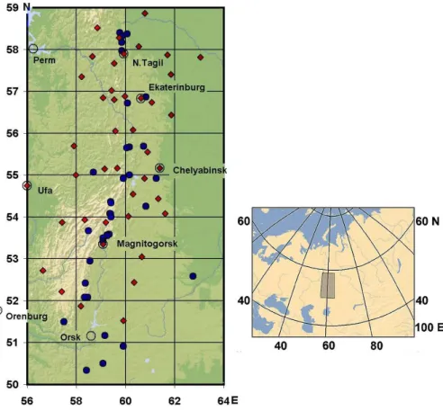
Fig. 1.Map of the studied region. Weather stations are shown as red rhombus, boreholes are shown as blue circles in the left panel. The right panel indicate the studied region position (grey trapezium) in Eurasia.
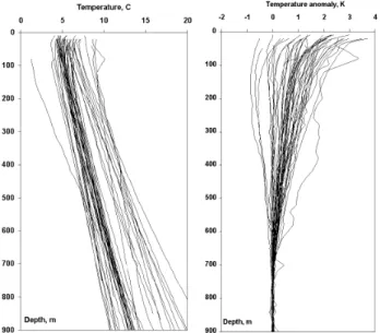
The left panel in Fig. 2 gives examples of borehole temper-ature logs included in the final sample. As the figure shows, the temperatures increase with depth almost linearly. Such temperature behaviour agrees with conductive heat transfer in thermally homogeneous media. Variations from the linear law are considered as temperature anomalies associated with climatically dependent variations of surface temperatures. A clearer understanding of the nature of these anomalies can be gained by reducing the measured borehole temperature logs (Fig. 2-right). The reducing procedure involves linear ap-proximation of the lower section of a borehole temperature log (bearing interval) by the least-squares method, extrapo-lation of the linear trend to the earth surface, and computation of the difference between measured and extrapolated temper-atures. To standardise the interpretation procedure we used an identical bearing interval of 720–900 m for all the bore-hole temperature logs.
A reconstruction of ground surface temperature histories (GSTH) for each borehole temperature log was obtained by solving the heat conduction boundary problem for thermally homogeneous media in relation to unknown parameters of the boundary condition at the surface. The algorithm of bore-hole temperature inversion, used in this study (Demezhko and Shchapov, 2001), allows reconstructions of GSTH as a
step function with uneven time intervals: the duration of the intervals increase into the past. The pattern of reconstructed GSTHs looks much the same (Fig. 3): all reconstructions have temperature minima between 1600 and 1900 yrs and temperature maxima between 800 and 1700 yrs. The max-ima approxmax-imately correlate with the Medieval Warm Period (MWP), and the minima with the Little Ice Age (LIA). How-ever, dates of the extremes vary. There are two principal causes for disagreement of the extremes: i) joint influence of a number of non-climatic causes (ground water flow, surface relief, changes in vegetation and snow cover); and ii) vari-ations of mean rock thermal diffusivity from one borehole to another. The coefficient of thermal diffusivitya dictates the rate of thermal wave propagation into rocks. In fact, the history argument is not time but the product ofa×t, where
tis the time interval between the climatic event and the date of thermal logging (years ago). A single value of the coeffi-cient of thermal diffusivity is generally used in the palaeocli-matic analysis of several borehole temperature logs. In our case we took the mean for crystalline rocks of the Urals to bea=10−6m2/s (Demezhko, 2001; Golovanova, 2005). The
Fig. 2. Borehole temperature logs used in this study (left) and temperature anomalies calculated by reducing borehole temperature logs (right).
the reconstructed temperature history is the sum of the true history over the time scale (extended linearly in an arbitrary manner) and low-frequency noise.
To obtain the regional characteristic of GSTH we used the interval estimates method proposed by Demezhko et al. (2005), who showed that traditional averaging of individ-ual GSTHs (minimum estimate) yield significantly underes-timated amplitudes. Maximum estimates take into account the real position of minima and maxima identified as LIA and MWP on the time scale. Ignoring the presence of non-climatic noise in the initial data makes the maximum esti-mate too high. The optimum estiesti-mate curve lies between minimum and maximum estimates and its position depends on the signal-to-noise ratio in the initial data. In our case the signal-to-noise ratio is equal to 1.25 and the optimal GSTH curve is close to the maximal estimate (Fig. 3).
Uncertainties in the averaged curve (minimum estimate) may be characterized by the standard error of the mean for any time cross-section, which is 7 times (root square of 49 – number of reconstruction) less than the standard deviation of temperature. Vertical lines in Fig. 3 cover the interval “mean temperature ±double standard error of mean”, which ap-proximately provide a 95% confidence limit. Although in-dividual reconstructions differ substantially, the standard er-ror of the mean does not exceed 0.12 K. Differences between minimum and maximum estimates are larger (0.5 K for LIA and 0.35 for MWP), and determine the main interval of un-certainty. The optimum curve presents the most probable his-tory within the main interval of uncertainty.
The optimal GSTH has sufficiently higher amplitude of temperature variation than the same obtained earlier by the
Fig. 3.Reconstructions of the GSTH. Pale curves denote individual reconstructions; blue -averaged history (minimum estimate; verti-cal lines denote±double standard error of mean: red – maximum estimate; black – optimum estimate.
partially overlapped sample of geothermal data (Pollack et al., 2003). For example, the temperature difference between 1720 and 1960 AD in the Urals according to (Pollack et al., 2003) is about 0.7 K – two times less than the optimal esti-mate. There are a number of reasons for such disagreement: the mentioned paper used temperature profiles of less depth, the choice of reconstruction parameters, and the traditional averaging of individual GSTHs.
Under usual averaging of the GSTH curves applied by a number of researchers (Tyson et al., 1998; Pollack et al., 2003; Pollack and Smerdon, 2004) non-correlated noise is efficiently eliminated. In doing so the true amplitude is also reduced, i.e. the estimate of the mean temperature history is too low. In such cases an optimum procedure can be em-ployed for deriving interval estimates of temperature ampli-tudes. Such estimates can be derived, provided that either non-climatic noise or variations in temperature diffusivity are taken into account separately.
3 Meteorological data
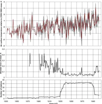
Fig. 4. Reduced air surface mean annual temperatures recorded in weather stations in the Middle and South Urals (pale curves in the upper panel). The averaged record is shown with a bold red line. The middle panel presenting standard error of mean, the bottom panel – the number of weather stations with the data on each time interval.
To evaluate regional variability of mean annual air tem-peratures we used the averaging procedure that takes into account the differences in the length of records and in the temperature constant – a latitudinal trend (Hansen and Lebe-deff, 1987). Before averaging, each record was reduced by subtracting an individual value of temperature, the anomaly records were then averaged in the usual manner (Fig. 4). No homogeneity tests were performed. For the period 1890– 1930 the standard error of the mean was about 0.2 K, then it decreases to 0.05 K (1935–1990), and increases again in the last decade of the century. The total standard deviation of averaged mean annual air surface temperatures is about 1 K. A synchronous pattern of the reduced records suggests that the eastern slope of the Middle and Southern Urals can be treated as a region of identical climatic history.
4 Analysis of geothermal evidence and meteorological data
Our comparative analysis is based upon two averaged datasets: surface air temperature over the past 170 years and the optimum estimation of ground surface temperature his-tory over the past 1200 years obtained from geothermal evi-dence. The obtained GSTH reconstruction supports the idea that natural variability during the last millennium may be
Fig. 5. Comparison of geothermal and meteorological data. Red curve – the reduced averaged record of air surface mean annual tem-peratures; blue curve – the same record smoothed out in the running 11-year interval; black curve – reconstructed ground surface tem-peratures (GSTH). The GSTH curve is slightly shifted along the temperature axis to enable an easier comparison.
larger than usually thought. This idea is also supported by a number of low-resolution proxies (including ice records, pollen and diatoms in lake sediments, foraminifers and sta-lagmites – see Moberg et al., 2005). According to pollen data the mean annual temperature in the MWP maximum (880– 1200) eastwards and westwards of the Urals was 0.7–0.2 K warmer than modern values (Klimenko, Klimanov, 2000). Reconstruction of upper treeline limit variations in the Polar Urals (Shiyatov, 2003) also shows that the upper timberline of larch in the 9–13 centuries was above its contemporary level, athough the treeline curve is shifted by 50–100 years (to the recent times) relative to the geothermal one. We hy-pothesize that it is caused by a delayed response of forest’s degradation/recovery to climate change.
The GSTH curve also may be directly compared with meteorological data (Fig. 5) during their period of overlap (1832–1985). The mean GSTH and air temperature rates of increase are approximately equal and come to 0.8 and 0.9 K per 100 years. A sharper temperature rise spanning the years 1970 to 1985 is also sufficiently reconstructed.
values. When analyzing the GSTH curve, one should bear in mind that geothermal information estimates temperatures averaged over increasingly longer periods back into the past. Any point on the GSTH curve (t, yrs ago) represents a tem-perature averaged over the periodt±t/3 yrs ago (Demezhko,
2001). Thus, the actual trend of cooling might be more com-plicated and interrupted repeatedly with occasional warming events. Warming begun after the temperature minimum in 1720 was also irregular. Warming averaged +0.25 K/100 yrs in the 18th century, +1.15 K/100 yrs in the 19th century, and +0.8 K/100 yrs in the first eighty-five years of the 20th cen-tury.
To estimate the average rates of air surface tempera-ture changes over periods of different duration we applied the method of linear approximation. The average rate of air temperature changes during the period 1930 to 2001 is +1.6 K/100 yrs. Interestingly, the average rate calculated in-dividually for weather stations near the larger cities (Nizhny Tagil, Ekaterinburg, Chelyabinsk, Ufa, Magnitogorsk, Oren-burg) is essentially not different from that in the entire data sample. This suggests that urban heat islands, which cer-tainly exist, are rather insignificant and do not affect air sur-face temperatures recorded at weather stations situated in the suburbs. One more interesting regional feature is revealed in the estimates of average rates in different latitudinal zones. From the south to the north the rates of warming decrease: 50–53◦N – +2.1 K/100 yrs, 53–56◦N – +1.6 K/100 yrs, 56– 59◦N – +1.4 K/100 yrs.
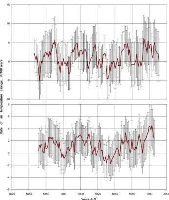
An idea of the temperature behaviour in time is given by the plots of slope coefficient of linear regression calcu-lated in the running intervals of different length (Fig. 6). As the length grows, the amplitudes of the rates show a regu-lar decrease. The sharpest warming took place during the 21-years periods 1963–1983 (+6.1 K/100 yrs), 1860–1880 (+5.7 K/100 yrs) and the other six intervals when the rates of warming were somewhat slower. The most anomalous 31-year periods fell on 1968–1998 (+4.5 K/100 yrs) and 1965– 1995 (+4.5 K/100 yrs). In this case the difference from pre-vious anomalies, with the rates of warming not more than +2.6–+3.4 K/100 yrs, seems to be wider. However, the con-fidence intervals calculated from thet-distribution (at 95% confidence), lies within±3 K/100 yrs. This makes the differ-ence of 1–1.5 K/100 yrs statistically insignificant.
Fig. 6. Slope coefficients of linear regression (average rates of air surface temperature variations) calculated in 21-year (top panel) and 31-year (bottom panel) running intervals. Vertical lines show 95% confidence intervals.
5 Conclusions
1. Geothermal evidence (borehole temperature logs) recorded in the Urals and the developed procedure of their interpretation enable the surface temperature his-tory over the last 1200 years to be reliably estimated. The obtained optimal GSTH estimate shows that natu-ral variability during the last millennium may be larger than usually thought. According to this estimation, sur-face temperature in the Medieval Warm Period (MWP) spanning 1100 and 1200 AD was 0.4 K warmer than the mean temperature of the 20th century (1900–1960) and surface temperature in the Little Ice Age in approxi-mately 1720 AD was 1.6 K cooler.
stracts, San Francisco, F842, 1998.
Beltrami, H. and Mareshal, J.-C.: Recent warming in eastern Canada inferred from geothermal measurements, Geophys. Res. Lett., 18, 4, 605–608, 1991.
Demezhko, D. Yu. and Shchapov, V. A.: 80,000 years ground sur-face temperature history inferred from the temperature-depth log measured in the superdeep hole SG-4 (the Urals, Russia), Global and Planetary Change, 29(1–2), 219–230, 2001.
Demezhko, D. Yu.: Geothermal method for palaeoclimate recon-structions (examples from the Urals, Russia), Ekaterinburg, UB RAS, 144 p., 2001 (in Russian).
Demezhko, D. Yu., Utkin, V. I., Shchapov, V. A., and Golovanova, I. V.: Variations in the Earth’s Surface Temperature in the Urals during the Last Millennium Based on Borehole Temperature Data, Doklady Earth Sciences, 403, 5, 764–766, 2005.
Golovanova, I. V., Harris, R. N., Selezniova, G. V., and ˇStulc, P.: Evidence of climatic warming in the southern Urals region de-rived from borehole temperatures and meteorological data, Glob. Planet. Change, 29, 167–188, 2001.
structed from borehole temperatures, J. Geophys. Res., 108(A4), 2180, doi:10.1029/2002JB002154, 2003.
Pollack, H. N. and Smerdon, J. E.: Borehole climate reconstruction: Spatial structure and hemispheric averages, J. Geophys .Res., 109, D11106, doi:10.1029/2003JD004163, 2004.
Smerdon, J. E., Pollack, H. N., Cermak V., Enz, J. W., Kresl, M., Safanda, J., and Wehmiller J. F.: Daily, seasonal, and annual re-lationships between air and subsurface temperatures, J. Geophys. Res., 111, D07101, doi:10.1029/2004JD005578, 2006.
ˇStulc, P., Golovanova, I. V., and Selezniova, G. V.: Climate Change in the Urals, Russia, inferred from Borehole Temperature Data, Studia Geoph. et Geod., 41, 225–246, 1997.
Shiyatov, S. G.: Rates of changes in the upper treeline ecotone in the Polar Ural Mountains, Pages Newsletter, 11(1), 8–10, 2003. Tyson, P. D., Mason, S. J., Jones, M. Q. W., and Cooper, G. R.