Small-scale variation of snow in a regional permafrost model

(1)

TCD

9, 6661–6696, 2015

Small-scale variation of snow in a regional permafrost model

K. Gisnås et al.

Title Page

Abstract Introduction

Conclusions References

Tables Figures

◭ ◮

Back Close

Full Screen / Esc

Printer-friendly Version Interactive Discussion

Discussion

P

a

per

|

Discussion

P

a

per

|

Discussion

P

a

per

|

Discussion

P

a

per

|

The Cryosphere Discuss., 9, 6661–6696, 2015 www.the-cryosphere-discuss.net/9/6661/2015/ doi:10.5194/tcd-9-6661-2015

This discussion paper is/has been under review for the journal The Cryosphere (TC). Please refer to the corresponding final paper in TC if available.

Small-scale variation of snow in a

regional permafrost model

K. Gisnås1, S. Westermann1, T. V. Schuler1, K. Melvold2, and B. Etzelmüller1

1

Department of Geosciences, University of Oslo, Oslo, Norway

2

Norwegian Water Resources and Energy Directorate, Oslo, Norway

Received: 10 November 2015 – Accepted: 18 November 2015 – Published: 8 December 2015

Correspondence to: K. Gisnås (kjersti.gisnas@geo.uio.no)

(2)

TCD

9, 6661–6696, 2015

K. Gisnås et al.

Title Page

Tables Figures

◭ ◮

Back Close

Full Screen / Esc

Discussion

P

a

per

|

Discussion

P

a

per

|

Discussion

P

a

per

|

Discussion

P

a

per

|

Abstract

The strong winds prevalent in high altitude and arctic environments heavily redistribute the snow cover, causing a small-scale pattern of highly variable snow depths. This has profound implications for the ground thermal regime, resulting in highly variable near-surface ground temperatures on the meter scale. Asymmetric snow distributions

5

combined with the non-linear insulating effect of snow also mean that the spatial aver-age ground temperature in a 1 km2area can not necessarily be determined based on the average snow cover for that area. Land surface or permafrost models employing a coarsely classified average snow depth will therefore not yield a realistic representation of ground temperatures. In this study we employ statistically derived snow distributions

10

within 1 km2grid cells as input to a regional permafrost model in order to represent sub-grid variability of ground temperatures. This is shown to improve the representation of both the average and the total range of ground temperatures: the model results show that we reproduce observed sub-grid ground temperature variations of up to 6◦C, with 98 % of borehole observations within the modelled temperature range. Based on this

15

more faithful representation of ground temperatures, we find the total permafrost area of mainland Norway to be nearly twice as large as what is modelled without a sub-grid approach.

1 Introduction

High altitude and arctic environments are exposed to strong winds and drifting snow

20

can create a small-scale pattern of highly variable snow depths. Seasonal snow cover is a crucial factor for the ground thermal regime in these areas (e.g. Goodrich, 1982; Zhang et al., 2001). This small-scale pattern of varying snow depths results in highly variable ground temperatures on the meter scale; up to 6◦C within areas of less than 1 km2 (Gisnås et al., 2014; Gubler et al., 2011). In general, grid-based numerical land

25

(3)

TCD

9, 6661–6696, 2015

K. Gisnås et al.

Title Page

Tables Figures

◭ ◮

Back Close

Full Screen / Esc

Discussion

P

a

per

|

Discussion

P

a

per

|

Discussion

P

a

per

|

Discussion

P

a

per

|

snow depths, and are not capable of representing such small-scale variability. For the Norwegian mainland, permafrost models have been implemented with a spatial grid resolution of 1 km2 (Gisnås et al., 2013; Westermann et al., 2013), and do therefore only represent the larger scale patterns of ground temperatures. As a consequence, they usually represent the lower limit of permafrost as a sharp boundary, where the

5

average ground temperature of a grid-cell crosses the freezing temperature (0◦C). In reality, the lower permafrost boundary is a fuzzy transition. Several local parameters, such as snow cover, solar radiation, vegetation, soil moisture and soil type cause a pro-nounced sub-grid variation of ground temperature. Different approaches have been developed to address this mismatch of scales, such as the TopoSub (Fiddes and

Gru-10

ber, 2012), which accounts for the variability of a range of surface parameters using

k-means clustering. At high latitudes, one of the principal controls on the variability of ground temperature is the effect of sub-grid variation in snow cover (Langer et al., 2013; Gisnås et al., 2013). Therefore procedures capable of resolving the small scale vari-ability of snow depths will have the potential to considerably improve the representation

15

of the ground thermal regime.

The spatial variation of snow during accumulation season is a result of several mech-anisms operating on di_fferent scales in di_fferent environments (Liston et al., 2004). In tundra and alpine areas, wind-affected deposition is the dominant control on the snow distribution at distances below 1 km (Clark et al., 2011). The coe_fficient of variation

20

(CV), defined as the ratio between the standard deviation and the mean, can be used as a measure of the extent of spread in a distribution. Previous studies suggest that the coe_fficient of variation of snow depths (CV_sd), typically ranging from low spread at 0.2 to high spread at 0.8, is well suited to reflect snow distributions in a range of environ-ments (e.g. Liston, 2004; Winstral and Marks, 2014). Liston (2004) assigned individual

25

(4)

TCD

9, 6661–6696, 2015

K. Gisnås et al.

Title Page

Tables Figures

◭ ◮

Back Close

Full Screen / Esc

Discussion

P

a

per

|

Discussion

P

a

per

|

Discussion

P

a

per

|

Discussion

P

a

per

|

a large number of snow surveys in the Northern Hemisphere shows a large spread of CV_sd values, in particular within this land use class, ranging from 0.1 to 0.9 (Clark et al., 2011). This illustrates the need for improved representation of snow distribution within this land use class.

An accurate representation of the small scale snow variation highly influences the

5

timing and magnitude of runoff in hydrological models, and a detailed picture of the sub-grid variability is of great value for the hydropower industry and in flood forecasting. Adequate representations of the snow covered fraction in land surface schemes are important for enhanced realism of simulated near surface air temperatures, ground temperatures and evaporation due to the considerable influence of snow cover on the

10

duration of melt season and the surface albedo.

In this study we derive functional dependencies between distributions of snow depth within 1 km_×1 km grid cells and CV_sd, based on an extensive in-situ data set from Norwegian alpine areas. In a second step, we employ the resulting snow distributions as input to the permafrost model CryoGRID1, a spatially distributed, equilibrium

per-15

mafrost model (Gisnås et al., 2013). From the sub-grid representation of ground tem-peratures, permafrost probabilities are derived, hence enabling a more realistic, fuzzy permafrost boundary instead of a binary, sharp transition. With this approach, we aim to improve permafrost distribution modelling in inhomogeneous terrains.

2 Setting

20

The model is implemented for the Norwegian mainland, extending from 58 to 71◦N. Both the topography and climate in Norway is dominated by the Scandes, the moun-tain range stretching south-north through Norway, separating the coastal western part with steep mountains and deep fjords from the eastern part where the mountains grad-ually decrease in height. The maritime climate of the west coast is dominated by

low-25

(5)

TCD

9, 6661–6696, 2015

K. Gisnås et al.

Title Page

Tables Figures

◭ ◮

Back Close

Full Screen / Esc

Discussion

P

a

per

|

Discussion

P

a

per

|

Discussion

P

a

per

|

Discussion

P

a

per

|

permafrost is present all the way to the southern parts of the Scandes, with a gradi-ent in the lower limit of permafrost from_∼1400 to 1700 m from east to west in central southern Norway, and from∼700 to 1200 m from east to west in northern Norway (Gis-nås et al., 2013). While permafrost is also found in mires at lower elevations both in southern and northern Norway, most of the permafrost is located in exposed terrain

5

above the tree line. This environment is dominated by strong winds resulting in heavy redistribution of snow.

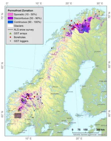
In-situ records of snow depth data used to establish the snow distribution scheme were collected at the Hardangervidda mountain plateau in the southern part of the Scandes (Fig. 1). It is the largest mountain plateau in northern Europe, located at

ele-10

vations from 1000 to above 1700 m a.s.l., with occurrences of permafrost in the highest mountain peaks. The terrain is open and slightly undulating in the east, while in the west it is more complex with steep mountains divided by valleys and fjords. The mountain range represents a significant orographic barrier for the prevailing westerly winds from the Atlantic Ocean, giving rise to large variations in precipitation and strong winds, two

15

agents promoting a considerably wind-affected snow distribution. Mean annual precipi-tation varies from 500 to more than 3000 mm over distances of a few tens of kilometres, and maximum snow depths can vary from zero to more than 10 m over short distances (Melvold and Skaugen, 2013).

3 Model description

20

3.1 A statistical model for snow depth variation

The Winstral terrain-based approach (Winstral et al., 2002) is applied over the entire Norwegian mainland using the 10 m national digital terrain model from the Norwegian Mapping Authority (available at Statkart.no), with wind data from the NORA10 dataset (Sect. 4.1) used to indicate the distribution of prevailing wind directions during

accu-25

(6)

TCD

9, 6661–6696, 2015

K. Gisnås et al.

Title Page

Tables Figures

◭ ◮

Back Close

Full Screen / Esc

Discussion

P

a

per

|

Discussion

P

a

per

|

Discussion

P

a

per

|

Discussion

P

a

per

|

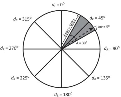
The terrain-based exposure parameter (Sx), described in detail in Winstral et al. (2002), quantifies the extent of shelter or exposure of the grid-cell considered.

Sxis determined by the slope between the grid-cell and the cells of greatest upward slope in the upwind terrain. The upwind terrain is defined as a sector towards the pre-vailing wind directiond constrained by the maximum search distance (d_max=100 m)

5

and a chosen width (A) of 30◦ with the two azimuths extending 15◦ to each side of d

(see Fig. 2). The cell of the maximum upward slope is identified for each search vec-tor, separated by 5◦ increments. Sx for the given grid-cell is finally calculated as the average of the maximum upward slope gradient of all seven search vectors:

Sx_d_,_A_,_d_max(x_iy_i)=max

tan

_Z₍_x

v,yv)−Z(xi,yi)

[(xv−xi)2+(yv−yi)2]0.5

(1)

10

whered is the prevailing wind direction, (x_i,y_i) are the coordinates of the considered grid-cell, and (x_v,y_v) are the sets of all cell coordinates located along the search vector defined by (xi, yi), A and dmax. This gives the degree of exposure or shelter in the

range₋1 to 1, where negative values indicate exposure.

To estimate a realistic degree of exposure based on the observed wind pattern

15

at a local site, Sx was computed for each of the eight prevailing wind directions

d=[0, 45, 90, 135, 180, 225, 270, 315◦], and weighted based on the wind fraction (wf_d). wf_d accounts for the amount of different exposures in the terrain at various wind direc-tions, and represents the fraction of hourly wind direction observations over the accu-mulation season for the eight wind directions. The accuaccu-mulation season is here chosen

20

as January to March. Wind speeds below a threshold of 7 ms−1 are excluded, as this threshold is considered a lower limit required for wind drifting of dry snow (Lehning and Fierz, 2008; Li and Pomeroy, 1997).

The calculated Sx parameter values are used as predictors in different regression analyses to describe the CV_sdwithin 1 km_×1 km derived from the ALS. The coefficient

25

(7)

TCD

9, 6661–6696, 2015

K. Gisnås et al.

Title Page

Tables Figures

◭ ◮

Back Close

Full Screen / Esc

Discussion

P

a

per

|

Discussion

P

a

per

|

Discussion

P

a

per

|

Discussion

P

a

per

|

CV_Sx=std(eSx)/mean(eSx). (2)

Sxvalues below the 2.5th and above 97.5th percentiles of theSxdistributions are ex-cluded, givingSx≈[−0.2, 0.2]. Three regression analyses were performed to reduce the RMSE between CV_Sx and observed CV_sd, where additional predictors such as elevation above treeline (z) and maximum snow depth (µ) successively have been

in-5

cluded (Table 1). Elevation above treeline is chosen as predictor to account for the increased wind exposure with elevation. Ideally, wind speed should be included as pre-dictor. However, the NORA10 dataset (Sect. 4.1) does not su_fficiently reproduce the local variations in wind speeds over land, especially not at higher elevations and for terrain with increased roughness. Because of the strong gradient in treeline and

gen-10

eral elevation of mountain peaks from high mountains in the south to lower topography in the north of Norway, applying only elevation as predictor would result in an underes-timation of redistribution in the north.

3.2 CryoGRID 1 with an integrated sub-grid scheme for snow variation

The equilibrium permafrost model CryoGRID 1 (Gisnås et al., 2013; Westermann et al.,

15

2015) provides an estimate for the MAGST (Mean annual ground surface temperature) and MAGT (Mean Annual Ground Temperature) from freezing (FDD_a) and thawing (TDD_a) degree days in the air according to

MAGST=TDDa ×nT−FDDa×nF

P (3)

and

20

MAGT=







(TDDa·nT_·r_k₋FDDa·nF)

P forKtTDDs≤KfFDDs

TDDa·nT₋1

rk·FDDa·nF

P forKtTDDs≥KfFDDs

(8)

TCD

9, 6661–6696, 2015

K. Gisnås et al.

Title Page

Tables Figures

◭ ◮

Back Close

Full Screen / Esc

Discussion

P

a

per

|

Discussion

P

a

per

|

Discussion

P

a

per

|

Discussion

P

a

per

|

whereP is the period that FDD_aand TDD_aare integrated over,rkis the ratio of thermal

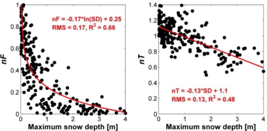
conductivities of the ground in thawed and frozen states, whilenT and nF are semi-empirical transfer-functions including a variety of processes in one single variable.

The winternFfactor relates the freezing degree days at the surface to the air and thus accounts for the e_ffect of the winter snow cover, and likewise thenTfactor relates the

5

thawing degree days at the surface to the air and accounts for the surface vegetation cover:

FDD_s=nF ·FDD_aand TDD_s=nT·TDD_a. (5)

Variation in observednfactors for forests and shrubs are relatively small, withnT fac-tors typically in the range 0.85 to 1.1, andnF factors in the range 0.3 to 0.5 (Gisnås

10

et al., 2013). Following Gisnås et al. (2013) forest, shrubs and mires are assigned

nTfactors 0.9/1.0/0.85 andnFfactors 0.4/0.3/0.6, respectively.

Observed variations innTandnFwithin the open non-vegetated areas are compa-rably large, with values typically in the range 0.4–1.2 fornT and 0.1–1.0 for nF. The variability is related to the high impact and high spatial variability of snow depths

(Gis-15

nås et al., 2014). WhilenF accounts for the insulation from snow due to low thermal conductivity,nTindirectly compensates for the shorter season of thawing degree days at the ground surface in areas with a thick snow cover. Relationships betweennfactors for open areas and maximum snow depths are established based on air and ground temperature observations together with snow depth observations at the end of

accu-20

mulation season at the 13 stations in southern Norway, presented in Hipp (2012) and at arrays of nearly 80 loggers at Finse and Juvvasshøe (Gisnås et al., 2014) (Fig. 3):

nF=−0.17·ln(µ)+0.25 (6)

(9)

TCD

9, 6661–6696, 2015

K. Gisnås et al.

Title Page

Tables Figures

◭ ◮

Back Close

Full Screen / Esc

Discussion

P

a

per

|

Discussion

P

a

per

|

Discussion

P

a

per

|

Discussion

P

a

per

|

We assume that the distribution of maximum snow depths within a grid cell with a given CV_sdand average maximum snow depth (µ) follows agammadistribution with a prob-ability density function (PDF) given by:

f(x;α,β)= 1

βα_Γ₍_α₎x

α−1_e−xβ ₍₈₎

with ashapeparameterα=CV−_sd2and arateparameterβ=µ_×CV2_sd(e.g. Kolberg and

5

Gottschalk, 2006; Skaugen et al., 2004). Corresponding n factors are computed for all snow depths (x) based on Eqs. (6) and (7), and related to the PDF (Eq. 8). The model is run for eachnFfrom 0 to 1 with 0.01 spacing, giving 100 model realizations. Each realization corresponds to a unique snow depth, represented with a set of nF

andnTfactors. Based on the 100 realizations a distribution of MAGST and MAGT are

10

calculated for each grid cell, where the potential permafrost fraction is derived as the percentage of sub-zero MAGT. To assess the sensitivity of the choice of the theoretical distribution function, the model was also run with PDFs following alognormal distribu-tion, given by (e.g. Liston, 2004):

f(x;λ,ζ)= 1

xζ√2e

−12

h_ln(_x₎

−λ ζ

i2

(9)

15

where

λ=ln(µ)₋1 2ζ

2_, _ζ2

=ln(1₊CV_sd). (10)

3.3 Model evaluation

The CV_sd was derived for 0.5 km×1 km areas based on the ALS snow depth data (Sect. 4.1) resampled to 10 m_×10 m resolution. Each 0.5 km_×1 km area includes 500

20

(10)

TCD

9, 6661–6696, 2015

K. Gisnås et al.

Title Page

Tables Figures

◭ ◮

Back Close

Full Screen / Esc

Discussion

P

a

per

|

Discussion

P

a

per

|

Discussion

P

a

per

|

Discussion

P

a

per

|

of fit evaluations for the theoretical lognormal and gamma distributions applying the Anderson–Darling test in MATLB (adtest.m, Stephens, 1974) were conducted for each distribution. Parameters for gamma (shapeandrate) and lognormal (mu,sigma) distri-butions were estimated by maximum likelihood as implemented in the MATLAB func-tions gamfit.m and lognfit.m.

5

The results of the permafrost model are evaluated with respect to the average MAGST and MAGT within each grid cell, as well as the fraction of sub-zero MAGST. The model runs are forced with climatic data for the hydrological year corresponding to the observations. The performance in representing fractional permafrost distribu-tion is evaluated at two field sites where arrays of 26 (Juvvasshøe) and 41 (Finse)

10

data loggers have measured the distribution of ground surface temperatures within 500 m×500 m areas for the hydrological year 2013 (Gisnås et al., 2014). The general lower limits of permafrost are compared to permafrost probabilities derived from BTS (basal temperature of snow) – surveys (Haeberli, 1973; Lewkowicz and Ednie, 2004), conducted at Juvvasshøe and Dovrefjell (Isaksen et al., 2002). The model performance

15

of MAGST is evaluated with data from 128 temperature data loggers located a few cm below the ground surface in the period 1999–2009 (Farbrot et al., 2008, 2011, 2013; Isaksen et al., 2008, 2011; Ødegaard et al., 2008). The loggers represent all vegetation classes used in the model, and spatially large parts of Norway (Fig. 2). Four years of data from 25 boreholes (Isaksen et al., 2007, 2011; Farbrot et al., 2011, 2013) are used

20

to evaluate modelled MAGT (Fig. 2).

4 Data

4.1 Forcing and evaluation of the snow distribution scheme

Wind speeds and directions during the snow accumulation season are calculated from the boundary layer wind speed and direction at 10 m in the Norwegian Reanalysis

25

(11)

TCD

9, 6661–6696, 2015

K. Gisnås et al.

Title Page

Tables Figures

◭ ◮

Back Close

Full Screen / Esc

Discussion

P

a

per

|

Discussion

P

a

per

|

Discussion

P

a

per

|

Discussion

P

a

per

|

ERA-40 to a spatial resolution of 10–11 km, with hourly resolution of wind speed and direction (Reistad et al., 2011). The dataset is originally produced for wind fields over sea, and underestimates the wind speeds at higher elevation over land (Haakenstad et al., 2012). Comparison with weather station data revealed that wind speeds above the tree line are underestimated by about 60 % (Haakenstad et al., 2012). For these

5

areas the forcing dataset has been scaled accordingly.

The snow distribution scheme is derived from an Airborne Laser Scanning (ALS) snow depth over the Hardangervidda mountain plateau in southern Norway (Melvold and Skaugen, 2013). The ALS scan is made along six transects, each covering a 0.5 km_×80 km area. The survey was first conducted between 3 and 21 April 2008,

10

and repeated in the period 21–24 April 2009. The snow cover was at a maximum dur-ing both surveys. A baseline scan was performed 21 September 2008 to obtain the elevation at minimum snow cover. The ASL data are presented in detail in Melvold and Skaugen (2013). Distributions of snow depth, represented as CV_sd, are calculated for each 0.5 km_×1 km area, based on the snow depth data resampled to 10 m_×10 m

reso-15

lution. About 400 cells of 0.5 km_×1 km exist for each year, when lakes and areas below treeline are excluded.

The snow distribution scheme is validated with snow depth data obtained by ground penetrating radar (GPR) at Finse (60◦34′N, 7◦32′E, 1250–1332 m a.s.l.) and Juvvasshøe (61◦41′N, 8◦23′E, 1374–1497 m a.s.l.). The two field sites are both located

20

in open, non-vegetated alpine landscapes with major wind re-distribution of snow. How-ever, they differ with respect to elevation (1300/1450 m a.s.l.), mean maximum snow depth (_∼2 m/_∼1 m), average winter wind speeds (7–8/10–14 m s−1) and topography (very rugged at Finse, while steep, but less rugged at Juvvasshøe). The timing of the snow surveys were late March to April (2009, 2012–2014) around maximum snow

25

(12)

TCD

9, 6661–6696, 2015

K. Gisnås et al.

Title Page

Tables Figures

◭ ◮

Back Close

Full Screen / Esc

Discussion

P

a

per

|

Discussion

P

a

per

|

Discussion

P

a

per

|

Discussion

P

a

per

|

other years are obtained and processed following the same procedures, described in detail in Dunse et al. (2009). The propagation speed of the radar signal in dry snow was derived from the permittivity and the speed of light in vacuum, with the permittiv-ity obtained from snow denspermittiv-ity using an empirical relation (Kovacs et al., 1995). The snow depths were determined from the two-way travel time of the reflection from the

5

ground surface and the wave-speed. Observations were averaged over 10 m×10 m grid cells, where grid cells containing less than three samples were excluded. The CV_sdfor 1 km_×1 km areas are computed based on the 10 m resolution data.

4.2 Permafrost model setup

The climatic forcing of the permafrost model is daily gridded air temperature and snow

10

depth data for the period 1961–2013, called theseNorgedataset, provided by the Nor-wegian Meteorological Institute (Mohr and Tveito, 2008; Mohr, 2009) and the Norwe-gian Water and Energy Directorate (Engeset et al., 2004; Saloranta, 2012). The dataset is based on air temperature and precipitation data collected at the official meteorologi-cal stations in Norway, interpolated to 1 km_×1 km resolution. Snow depths are derived

15

from the air temperature and precipitation data, using a snow algorithm accounting for snow accumulation and melt, temperature during snow fall and compaction. Freezing (FDD_a) and thawing (TDD_a) degree days in the air are calculated as annual accumu-lated negative (FDD) and positive (TDD) daily mean air temperatures, and maximum annual snow depths (µ) are derived directly from the daily gridded snow depth data.

20

The CryoGRID 1 model is implemented at 1 km_×1 km resolution over the same grid as theseNorgedataset.

Soil properties and surface cover is kept as in Gisnås et al. (2013), with five land cover classes; forest, shrubs, open non-vegetated areas, mires and no data, based on CLC level 2 in the Norwegian Corine Land Cover map 2012 (Aune-Lundberg and

25

(13)

TCD

9, 6661–6696, 2015

K. Gisnås et al.

Title Page

Tables Figures

◭ ◮

Back Close

Full Screen / Esc

Discussion

P

a

per

|

Discussion

P

a

per

|

Discussion

P

a

per

|

Discussion

P

a

per

|

5 Results

5.1 Observed snow distributions in mountain areas of Norway

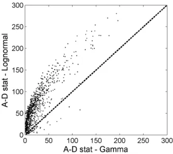
CV_sdwithin 1 km_×1 km areas in the ALS snow survey at Hardangervidda ranged from 0.15 to 1.14, with mean and median of respectively 0.58 and 0.59. According to the Anderson–Darling goodness of fit evaluations 70 out of 932 areas had a snow

distri-5

bution within the 5 % significance interval of agamma distribution, while only 1 area was within the 5 % significance interval of alognormal distribution. Although the null hypothesis rejected more than 90 % of the sample distributions, the Anderson–Darling Test Score was all over lower for thegammadistribution, indicating that the observed snow distributions are closer to a gammathan to a lognormal theoretical distribution

10

(Fig. 4). For lower lying areas with less varying topography and shallower snow depths, in particular in the eastern parts of Hardangervidda, the observed snow distributions were similarly close to alognormalas to agammadistribution. In higher elevated parts with more snow to the west of the plateau the snow distributions were much closer to agammadistribution. Based on these findings agammadistribution was used in the

15

main model runs, while a model run withlognormaldistributions of snow was made to evaluate the sensitivity towards the choice of the distribution function (Sect. 3.2).

5.2 Evaluation of the snow distribution scheme

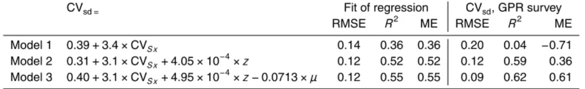
Three regression models for CV_sd as a function of the terrain-based parameter Sx, elevation (z) and mean maximum snow depth (µ) were calibrated with the snow

dis-20

tribution data from the ALS snow survey over the Hardangervidda mountain plateau (Table 1). Model 1 results in a root mean square error (RMSE) of only 0.14, however, the correlations of the distributions are significantly improved by includingelevationas predictor (Model 2;R2=0.52). By includingmaximum snow depth as additional pre-dictor (Model 3) the model improves slightly to R2=0.55 (Fig. 5). The distribution of

25

(14)

TCD

9, 6661–6696, 2015

K. Gisnås et al.

Title Page

Tables Figures

◭ ◮

Back Close

Full Screen / Esc

Discussion

P

a

per

|

Discussion

P

a

per

|

Discussion

P

a

per

|

Discussion

P

a

per

|

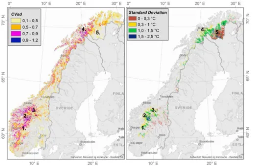
rougher topography (western side of Norway) and higher elevations (central part fol-lowing the Scandes), with maximum CV_sd up to 1.2 in the Lyngen Alps and at peaks around Juvvasshøe (Fig. 1, site 2 and 4). The lowest values of 0.2–0.3 are modelled in larger valleys in south eastern Norway, where elevations are lower and topography gentler.

5

The regression models for CV_sd are validated with data from GPR snow surveys at Juvvasshøe and Finse (Table 1). The correlation for Model 1 is poor, with R2=

0.04 and Nash–Sutcli_ffmodel e_fficiency (ME)₌₋0.7 (Table 1). Model 2 improves the correlation significantly, while the best fit is obtained with Model 3 (Fig. 5, RMSE=

0.094,R2=0.62 and ME=0.61). The improvement in Model 3 compared to Model 2

10

is more pronounced in the validation than in the fit of the regression models, and is mainly a result of better representation of the highest CV_sdvalues. The validation area at Juvvasshøe is located at higher elevations than what is represented in the ALS snow survey data set and undergoes extreme redistribution by wind. The representation of extreme values therefore has a high impact in the validation run.

15

5.3 Modelled ground temperatures for mainland Norway

The main results presented in this section are based on the model run with 100 realiza-tions per grid cell, applyinggammadistributions over the CV_sdfrom Model 3. According to the model run, in total 25 400 km2(7.8 %) of the Norwegian mainland is underlain by permafrost in an equilibrium situation with the climate over the 30-year period 1981–

20

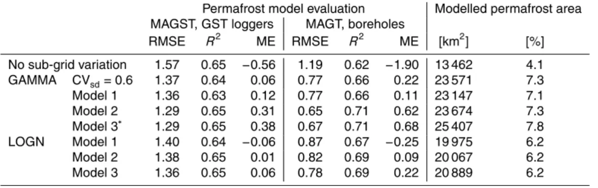
2010 (Fig. 1). 12 % of the land area features sub-zero ground temperatures in more than 10 % of a 1 km grid cell, and is classified as sporadic (4.4 %), discontinuous (3.2 %) or continuous (4.3 %) permafrost (Fig. 1). In comparison, the model run without a sub-grid variation results in a permafrost area of only 13 460 km2, corresponding to 4.1 % of the model domain (Table 2). The difference is illustrated for Juvvasshøe (Fig. 6a) and

25

(15)

TCD

9, 6661–6696, 2015

K. Gisnås et al.

Title Page

Tables Figures

◭ ◮

Back Close

Full Screen / Esc

Discussion

P

a

per

|

Discussion

P

a

per

|

Discussion

P

a

per

|

Discussion

P

a

per

|

model without sub-grid variability indicates a hard line for the permafrost limit at much higher elevations (Fig. 6b and d). At Juvvasshøe, the model without sub-grid distribu-tion still reproduces the permafrost limit to some extent because of the large elevadistribu-tion gradient. At Dovrefjell, where the topography is much gentler, the difference between the models is much larger and the approach without sub-grid distribution is not capable

5

of reproducing the observed permafrost distribution. The modelled permafrost area for model runs applying the other models for CV_sd and theoretical distribution functions are summarized in Table 2.

The standard deviations of the modelled sub-grid distribution of MAGT range from 0 to 2.5◦C (Fig. 7, right panel). The highest standard deviation values are found in the

10

Jotunheimen area, where modelled sub-grid variability of MAGT is up to 5◦C. Also at lower elevations in south eastern parts of Finnmark standard deviations exceed 1.5◦C. Here, the CV_sdvalues are below 0.4, but because of cold (FDD_a<₋2450◦C) and dry (max SD<0.5 m) winters even small variations in the snow cover result in large e_ffects on the ground temperatures.

15

Close to 70 % of the modelled permafrost is situated within open, non-vegetated areas above treeline, classified as mountain permafrost according to Gruber and Hae-berli (2009). This is the major part of the permafrost extent both in northern and south-ern Norway. In northsouth-ern Norway the model results indicate that the lower limit of con-tinuous/sporadic mountain permafrost decreases eastwards from 1200/700 m a.s.l.,

re-20

spectively, in the west to 500/200 m in the east. In southern Norway, the southern-most location of continuous mountain permafrost is in the mountain massif of Gaus-tatoppen at 59.8◦N, with continuous permafrost above 1700 m a.s.l. and discontinu-ous permafrost down to 1200 m a.s.l. In more central southern Norway the continudiscontinu-ous mountain permafrost reaches down to 1600 m a.s.l. in the western Jotunheimen and

25

(16)

TCD

9, 6661–6696, 2015

K. Gisnås et al.

Title Page

Tables Figures

◭ ◮

Back Close

Full Screen / Esc

Discussion

P

a

per

|

Discussion

P

a

per

|

Discussion

P

a

per

|

Discussion

P

a

per

|

5.4 Evaluation of CryoGRID 1 with sub-grid snow distribution scheme

The observed and modelled CV_sd values at the field sites were 0.85 and 0.80 at Juvvasshøe, and 0.71 and 0.77 at Finse. At Juvvasshøe the observed fraction of log-gers with MAGST below 0◦C was 77 %, while the model result indicates an aerial frac-tion of 64 %. Similarly, at Finse the observed negative MAGST fracfrac-tion was 30 %, while

5

the model indicates 32 %. The observed and modelled range in MAGST was [−1.8◦C, 1.0◦C] and [₋2.6◦C, 0.8◦C] at Juvvasshøe, and at Finse [₋1.9◦C, 2.7◦C] and [₋1.6◦C, 1.0◦_{C]. The average MAGSTs are}

−0.5/−0.5/0.8◦C (Juvvasshøe) and 0.8/0.2/1.3◦C (Finse) for observations, the sub-grid model and the model without sub-grid tempera-tures, respectively.

10

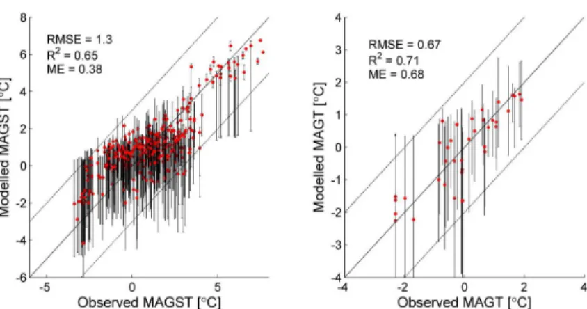
58 % of the observed MAGSTs are captured by the modelled range of MAGST for the corresponding grid cell, and 87 % within 1◦C outside the range given by the distribution. The overall correlation between observed MAGST and average modelled MAGST for a grid cell is fairly good with RMSE,R2and ME of 1.3◦C, 0.65 and 0.37, respectively (Fig. 8, left panel). The measured MAGT was within the range of modelled MAGT in

15

all boreholes except of one, this being 0.2◦C outside the range. All the average mod-elled MAGT are within_±1.6◦C of observations, while 90 % are within 1◦C. The RMSE between the observed and modelled average MAGT is 0.6◦C (Fig. 8, right panel).

The evaluation of the model runs with all three CV_sd-models, as well as lognormal

instead ofgammadistribution functions are summarized in Table 2. The highest

corre-20

lation between observed and mean MAGST and MAGT was obtained by Model 3, but Model 2 yielded similar correlations. All three model runs capture 58 % of the observed MAGST and more than 98 % of the observed MAGT within the temperature range of the corresponding grid cell. The total area of modelled permafrost is 9 % less when ap-plying the simplest snow distribution model (Model 1) compared to the reference model

25

(17)

TCD

9, 6661–6696, 2015

K. Gisnås et al.

Title Page

Tables Figures

◭ ◮

Back Close

Full Screen / Esc

Discussion

P

a

per

|

Discussion

P

a

per

|

Discussion

P

a

per

|

Discussion

P

a

per

|

6 Discussion

6.1 The e_ffect of a statistical representation of sub-grid variability in a regional permafrost model

The total distribution of modelled permafrost with the sub-grid snow scheme corre-sponds to 7.8 % of the Norwegian land area, while the modelled permafrost area

with-5

out a sub-grid representation of snow is_∼4 %. This large di_fference in total modelled permafrost area stems exclusively from di_fferences in the amount of modelled per-mafrost in mountains above the treeline. In these areas the snow distribution is highly asymmetric with a majority of the area having below average snow depths. Because of the non-linearity in the insulating e_ffect of snow cover the mean ground temperature of

10

a grid cell is not, and is often far from, the same as the ground temperature below the average snow depth. Often, the majority of the area in high, wind exposed mountains is nearly bare blown with most of the snow blown into terrain hollows. Consequently, most of the area experiences significantly lower average ground temperatures than with an evenly distributed, average depth snow cover. In mountain areas with a more gentle

to-15

pography and relatively small spatial temperature variations, an evenly distributed snow depth will result in large biases in modelled permafrost area, as illustrated at Dovrefjell in Fig. 6. This study is clear evidence that the sub-grid variability of snow depths should be accounted for in model approaches targeting the ground thermal regime and per-mafrost distribution.

20

The model reproduces the large range of variation in sub-grid ground temperatures, with standard deviations up to 2.5◦C. This is in accordance with the observed small-scale variability of up to 6◦C within a single grid cell (Gisnås et al., 2014; Gubler et al., 2011). Inclusion of sub-grid variability of snow depths in model approaches allows for a more adequate representation of the gradual transition from permafrost

25

(18)

TCD

9, 6661–6696, 2015

K. Gisnås et al.

Title Page

Tables Figures

◭ ◮

Back Close

Full Screen / Esc

Discussion

P

a

per

|

Discussion

P

a

per

|

Discussion

P

a

per

|

Discussion

P

a

per

|

blown areas with mean annual ground temperatures of₋6◦C need a large tempera-ture increase to thaw. Increased precipitation as snow would also warm the ground; however, bare blown areas may still be bare blown with increased snow accumula-tion during winter. A statistical snow distribuaccumula-tion reproduces this e_ffect, also with an increase in mean snow depth.

5

CryoGRID1 is a simple modelling scheme delivering a mean annual ground tempera-ture at the top of the permanently frozen ground based on near-surface meteorological variables, under the assumption that the ground thermal regime is in equilibrium with the applied surface forcing. This is a simplification, and the model cannot reproduce the transient evolution of ground temperatures. However, it has proven to capture the

re-10

gional patterns of permafrost reasonably well (Gisnås et al., 2013; Westermann et al., 2013). Because of the simplicity it is computationally efficient, and suitable for doing test-studies like the one presented in this paper and in similar studies (Westermann et al., 2015).

For the model evaluation with measured ground temperatures in boreholes

15

(Sect. 5.4), the modelled temperatures are forced with data for the hydrological year corresponding to the observations. Because of the assumption of an equilibrium situ-ation in the model approach, such a comparison can be problematic as many of the boreholes have undergone warming during the past decades. However, with the major-ity of the boreholes located in bedrock or coarse moraine material with relatively high

20

conductivity, the lag in the climate signal is relatively small at the depth of the top of permafrost.

The large amount of field observations used for calibration and evaluation in this study is mainly conducted in alpine mountain areas. The large spatial variation in win-ter snow depths is a major controlling factor also of the ground temperatures in peat

25

(19)

TCD

9, 6661–6696, 2015

K. Gisnås et al.

Title Page

Tables Figures

◭ ◮

Back Close

Full Screen / Esc

Discussion

P

a

per

|

Discussion

P

a

per

|

Discussion

P

a

per

|

Discussion

P

a

per

|

6.2 Model sensitivity

The sensitivity of the model for CV_sd to the modelled ground temperatures is rela-tively low, with only 9 % variation in permafrost area, although the performance of the snow distribution scheme varies significantly between the models when evaluated with GPR snow surveys (Table 1). In comparison, alognormalinstead of agamma

distribu-5

tion function reduces the permafrost area by 18 % (Table 2). The choice of distribution function therefore seems to be of greater importance than the fine tuning of a model for CV_sd. This result contradicts the conclusions by Luce and Tarboton (2004), suggesting that the parameterization of the distribution function is more important than the choice of distribution model. With a focus on hydrology and snow cover depletion curves, equal

10

importance was given to both the deeper and shallower snow depths in the mentioned study. In contrast, an accurate representation of the shallowest snow depths is crucial for modelling the ground thermal regime. The low thermal conductivity of snow results in a disconnection of ground surface and air temperatures at snow packs thicker than 0.5–1 m, depending on the physical properties of the snow pack (e.g. Haeberli, 1973).

15

In wind exposed areas prone to heavy redistribution, large fractions of the area will be entirely bare blown (Gisnås et al., 2014). These are the areas of greatest importance for permafrost modelling. In order to reproduce the gradual transition in the discontin-uous permafrost zone, where permafrost is often only present at bare blown ridges, shallow snow covers must be satisfactorily represented. Compared to agamma

func-20

tion, alognormaldistribution function to a larger degree underestimates the fraction of shallow snow depths, resulting in a less accurate representation of this transition.

Several studies include statistical representations of the sub-grid variability of snow in hydrological models, most commonly applying a two- or three-parameterlognormal

distribution (e.g. Pomeroy et al., 2004; Liston, 2004; Nitta et al., 2014; Donald et al.,

25

(20)

TCD

9, 6661–6696, 2015

K. Gisnås et al.

Title Page

Tables Figures

◭ ◮

Back Close

Full Screen / Esc

Discussion

P

a

per

|

Discussion

P

a

per

|

Discussion

P

a

per

|

Discussion

P

a

per

|

in non-forested alpine environments. However, the difference is not substantial in all areas; the two distributions can provide near-equal fit in eastern parts of the mountain plateau where the terrain is gentler and the wind speeds lower. We suggest that the choice of distribution function of snow is important in model applications for the ground thermal regime, and recommend the use ofgammadistribution for non-vegetated high

5

alpine areas prone to heavy redistribution of snow.

While a gammadistribution offers improvements over a lognormal distribution, the bare blown areas are still not su_fficiently represented. One attempt to solve this is to include a third parameter for the “snow free fraction” (e.g. Kolberg and Gottschalk, 2010; Kolberg et al., 2006). We made an attempt to calibrate such a parameter for this

10

study, however, no correlations to any of the predictors were found. It is also di_fficult to determine a threshold depth for “snow free” areas in ALS data resampled to 10 m resolution, where the uncertainty of the snow depth observations are in the order of ten centimetres (Melvold and Skaugen, 2013).

In this study a high number of realizations could be run per grid cell because of the

15

low computational cost of the model. To evaluate the sensitivity of sampling density, the number of realizations was reduced from 100 to 10 per grid cell. This resulted is a 2.6 % increase in total modelled permafrost area relative to the reference model run. This demonstrates that a statistical downscaling of ground temperatures as demonstrated in this study is robust and highly improves the model results with only a few additional

20

model realizations per grid cell.

7 Conclusions

We present a modelling approach to reproduce the variability of ground temperatures within the scale of 1 km2grid cells based on probability distribution functions over cor-responding seasonal maximum snow depths. The snow distributions are derived from

25

(21)

re-TCD

9, 6661–6696, 2015

K. Gisnås et al.

Title Page

Tables Figures

◭ ◮

Back Close

Full Screen / Esc

Discussion

P

a

per

|

Discussion

P

a

per

|

Discussion

P

a

per

|

Discussion

P

a

per

|

sults are evaluated with independent observations of snow depth distributions, ground surface temperature distributions and ground temperatures. From this study the follow-ing conclusions can be drawn:

– The model results indicate a total permafrost area of 25 400 km2, corresponding to 7.8 % of the Norwegian mainland, in an equilibrium situation with the average

5

climate over 1981–2010. 4 % of the model domain features permafrost for all snow depths.

– The same permafrost model without a sub-grid representation of snow produces almost 50 % less permafrost. Because of the non-linearity in the insulating e_ffect of snow cover in combination with the highly asymmetric snow distribution within

10

each grid cell, sub-grid variability of snow depths must be accounted for in models representing the ground thermal regime.

– Observed variations in ground surface temperatures from two logger arrays with 26 and 41 loggers, respectively, are very well reproduced, with estimated fractions of sub-zero MAGST within_±10 %. 94 % of the observed mean annual temperature

15

at top of permafrost in the boreholes are within the modelled ground temperature range for the corresponding grid cell, and mean modelled temperature of the grid cell reproduces the observations with an accuracy of 1.5◦C or better.

– The sensitivity of the model to the coefficient of variation of snow (CV_sd) is rela-tively low, compared to the choice of theoretical snow distribution function.

How-20

ever, both are minor e_ffects compared to the e_ffect of running the model without a sub-grid distribution.

– The observed CV_sdof snow within 1 km2grid cells in the Hardangervidda moun-tain plateau varies from 0.15 to 1.15, with an average CV_sd of 0.6. The distribu-tions are generally closer to a theoreticalgammadistribution than to alognormal 25

(22)

TCD

9, 6661–6696, 2015

K. Gisnås et al.

Title Page

Tables Figures

◭ ◮

Back Close

Full Screen / Esc

Discussion

P

a

per

|

Discussion

P

a

per

|

Discussion

P

a

per

|

Discussion

P

a

per

|

and higher average winter wind speeds. The observed CV_sd values are nearly identical at the end of the accumulation seasons in 2008 and 2009.

In areas subject to snow redistribution, the average ground temperature of a 1 km2grid cell must be determined based on the distribution, and not the overall average of snow depths within the grid cell. Furthermore, modelling the full range of ground

tempera-5

tures present over small distances enables representation of the gradual transition from permafrost to non-permafrost areas and most likely a more accurate response to cli-mate warming. This study is clear evidence that the sub-grid variability of snow depths should be accounted for in model approaches targeting the ground thermal regime and permafrost distribution.

10

Acknowledgements. This study is part of the CryoMet project (project number 214465; funded by the Norwegian Research Council). The field campaigns at Finse were partly founded by the hydropower companiesStatkraftandECO, while the field work at Juvvasshøe was done in collaboration with Ketil Isaksen (Norwegian Meteorological Institute). The Norwegian Meteoro-logical Institute provided the NORA10 wind data and theseNorgegridded temperature data. 15

The Norwegian Water and Energy Directorate provided theseNorgegridded snow depth data and the ALS snow survey at Hardangervidda. Kolbjørn Engeland gave valuable comments to the statistical analysis presented in the manuscript. We gratefully acknowledge the support of all mentioned individuals and institutions.

References

20

Aune-Lundberg, L. and Strand, G.-H.: CORINE Land Cover 2006, The Norwegian CLC2006 Project, Report from the Norwegian Forest and Landscape Institute 11/10, Norwegian Forest and Landscape Institute, Ås, Norway, 14 pp., 2010.

Clark, M. P., Hendrikx, J., Slater, A. G., Kavetski, D., Anderson, B., Cullen, N. J., Kerr, T., Hreinsson, E. Ö., and Woods, R. A.: Representing spatial variability of snow water equiv-25

(23)

TCD

9, 6661–6696, 2015

K. Gisnås et al.

Title Page

Tables Figures

◭ ◮

Back Close

Full Screen / Esc

Discussion

P

a

per

|

Discussion

P

a

per

|

Discussion

P

a

per

|

Discussion

P

a

per

|

Donald, J. R., Soulis, E. D., Kouwen, N., and Pietroniro, A.: A land cover-based snow cover representation for distributed hydrologic models, Water Resour. Res., 31, 995–1009, doi:10.1029/94WR02973, 1995.

Dunse, T., Schuler, T. V., Hagen, J. O., Eiken, T., Brandt, O., and Høgda, K. A.: Recent fluctua-tions in the extent of the firn area of Austfonna, Svalbard, inferred from GPR, Ann. Glaciol., 5

50, 155–162, doi:10.3189/172756409787769780, 2009.

Engeset, R., Tveito, O. E., Alfnes, E., Mengistu, Z., Udnæs, C., Isaksen, K., and Førland, E. J.: Snow map system for Norway, in: NHP Report 48, XXIII Nordic Hydrological Conference, 8–12 August 2004, Tallin, Estonia, 2004.

Farbrot, H., Isaksen, K., and Etzelmüller, B.: Present and past distribution of mountain per-10

mafrost in Gaissane Mountains, Northern Norway, in: Proceeding of the Ninth International Conference on Permafrost, Fairbanks, Alaska, 427–432, 2008.

Farbrot, H., Hipp, T. F., Etzelmüller, B., Isaksen, K., Ødegård, R. S., Schuler, T. V., and Hum-lum, O.: Air and ground temperature variations observed along elevation and continental-ity gradients in Southern Norway, Permafrost Periglac., 22, 343–360, doi:10.1002/ppp.733, 15

2011.

Farbrot, H., Isaksen, K., Etzelmüller, B., and Gisnås, K.: Ground thermal regime and permafrost distribution under a changing climate in Northern Norway, Permafrost Periglac., 24, 20–38, doi:10.1002/ppp.1763, 2013.

Fiddes, J. and Gruber, S.: TopoSUB: a tool for efficient large area numerical modelling in com-20

plex topography at sub-grid scales, Geosci. Model Dev., 5, 1245–1257, doi:10.5194/gmd-5-1245-2012, 2012.

Gisnås, K., Etzelmuller, B., Farbrot, H., Schuler, T. V., and Westermann, S.: CryoGRID 1.0: Per-mafrost distribution in Norway estimated by a spatial numerical model, PerPer-mafrost Periglac., 24, 2–19, doi:10.1002/ppp.1765, 2013.

25

Gisnås, K., Westermann, S., Schuler, T. V., Litherland, T., Isaksen, K., Boike, J., and Et-zelmüller, B.: A statistical approach to represent small-scale variability of permafrost tem-peratures due to snow cover, The Cryosphere, 8, 2063–2074, doi:10.5194/tc-8-2063-2014, 2014.

Goodrich, L. E.: The influence of snow cover on the ground thermal regime, Can. Geotech. J., 30

19, 421–432, 1982.

(24)

TCD

9, 6661–6696, 2015

K. Gisnås et al.

Title Page

Tables Figures

◭ ◮

Back Close

Full Screen / Esc

Discussion

P

a

per

|

Discussion

P

a

per

|

Discussion

P

a

per

|

Discussion

P

a

per

|

Gubler, S., Fiddes, J., Gruber, S., and Keller, M.: Scale-dependent measurement and analysis of ground surface temperature variability in alpine terrain, The Cryosphere Discuss., 5, 307– 338, doi:10.5194/tcd-5-307-2011, 2011.

Haakenstad, H., Reistad, M., Haugen, J. E., and Breivik, Ø.: Update of the NORA10 hindcast archive for 2011 and study of polar low cases with the WRF model, met.no report 17/2012, 5

Norwegian Meteorological Institute, Oslo, 2012.

Haeberli, W.: Die Basis-Temperatur der winterlichen Schneedecke als möglicher Indikator für die Verbreitung von Permafrost in den Alpen, Z. Gletscherk. Glazialgeol., 9, 221–227, 1973. Hipp, T.: Mountain Permafrost in Southern Norway. Distribution, Spatial Variability and Impacts

of Climate Change, PhD thesis, Faculty of Mathematics and Natural Sciences, Department 10

of Geosciences, University of Oslo, Oslo, 166 pp., 2012.

Isaksen, K., Hauck, C., Gudevang, E., Ødegård, R. S., and Sollid, J. L.: Mountain permafrost distribution in Dovrefjell and Jotunheimen, southern Norway, based on BTS and DC resistivity tomography data, Norsk Geogr. Tidsskr., 56, 122–136, doi:10.1080/002919502760056459, 2002.

15

Isaksen, K., Sollid, J. L., Holmlund, P., and Harris, C.: Recent warming of mountain permafrost in Svalbard and Scandinavia, J. Geophys. Res., 112, F02S04, doi:10.1029/2006jf000522, 2007.

Isaksen, K., Farbrot, H., Blikra, L., Johansen, B., Sollid, J., and Eiken, T.: Five year ground surface temperature measurements in Finnmark, Northern Norway, in: Ninth International 20

Conference on Permafrost, Fairbanks, Alaska, 789–794, 2008.

Isaksen, K., Ødegård, R. S., Etzelmüller, B., Hilbich, C., Hauck, C., Farbrot, H., Eiken, T., Hy-gen, H. O., and Hipp, T. F.: Degrading mountain permafrost in Southern Norway: spatial and temporal variability of mean ground temperatures, 1999–2009, Permafrost Periglac., 22, 361–377, doi:10.1002/ppp.728, 2011.

25

Kolberg, S. A. and Gottschalk, L.: Updating of snow depletion curve with remote sensing data, Hydrol. Process., 20, 2363–2380, 2006.

Kolberg, S. and Gottschalk, L.: Interannual stability of grid cell snow depletion curves as esti-mated from MODIS images, Water Resour. Res., 46, W11555, doi:10.1029/2008WR007617, 2010.

30

(25)

TCD

9, 6661–6696, 2015

K. Gisnås et al.

Title Page

Tables Figures

◭ ◮

Back Close

Full Screen / Esc

Discussion

P

a

per

|

Discussion

P

a

per

|

Discussion

P

a

per

|

Discussion

P

a

per

|

Kovacs, A., Gow, A. J., and Morey, R. M.: The in-situ dielectric constant of polar firn revisited, Cold Reg. Sci. Technol., 23, 245–256, doi:10.1016/0165-232X(94)00016-Q, 1995.

Langer, M., Westermann, S., Heikenfeld, M., Dorn, W., and Boike, J.: Satellite-based modeling of permafrost temperatures in a tundra lowland landscape, Remote Sens. Environ., 135, 12–24, doi:10.1016/j.rse.2013.03.011, 2013.

5

Lehning, M. and Fierz, C.: Assessment of snow transport in avalanche terrain, Cold Reg. Sci. Technol., 51, 240–252, doi:10.1016/j.coldregions.2007.05.012, 2008.

Lewkowicz, A. G. and Ednie, M.: Probability mapping of mountain permafrost using the BTS method, Wolf Creek, Yukon Territory, Canada, Permafrost Periglac., 15, 67–80, doi:10.1002/ppp.480, 2004.

10

Li, L. and Pomeroy, J. W.: Estimates of threshold wind speeds for snow trans-port using meteorological data, J. Appl. Meteorol., 36, 205–213, doi:10.1175/1520-0450(1997)036<0205:EOTWSF>2.0.CO;2, 1997.

Liston, G. E.: Representing subgrid snow cover heterogeneities in regional and global mod-els, J. Climate, 17, 1381–1397, doi:10.1175/1520-0442(2004)017<1381:RSSCHI>2.0.CO;2, 15

2004.

Luce, C. H. and Tarboton, D. G.: The application of depletion curves for parameterization of subgrid variability of snow, Hydrol. Process., 18, 1409–1422, doi:10.1002/hyp.1420, 2004. Melvold, K. and Skaugen, T.: Multiscale spatial variability of lidar-derived and

modeled snow depth on Hardangervidda, Norway, Ann. Glaciol., 54, 273–281, 20

doi:10.3189/2013AoG62A161, 2013.

Mohr, M.: Comparison of Versions 1.1 and 1.0 of Gridded Temperature and Precipitation Data for Norway, Norwegian Meteorological Institute, Oslo, 46 pp., 2009.

Mohr, M. and Tveito, O.: Daily temperature and precipitation maps with 1 km resolution de-rived from Norwegian weather observations, in: 13th Conference on Mountain Meteorol-25

ogy/17th Conference on Applied Climatology, Whistler, BC, Canada, 2008,

Nitta, T., Yoshimura, K., Takata, K., O’ishi, R., Sueyoshi, T., Kanae, S., Oki, T., Abe-Ouchi, A., and Liston, G. E.: Representing variability in subgrid snow cover and snow depth in a global land model: offline validation, J. Climate, 27, 3318–3330, doi:10.1175/JCLI-D-13-00310.1, 2014.

30

(26)

TCD

9, 6661–6696, 2015

K. Gisnås et al.

Title Page

Tables Figures

◭ ◮

Back Close

Full Screen / Esc

Discussion

P

a

per

|

Discussion

P

a

per

|

Discussion

P

a

per

|

Discussion

P

a

per

|

Pomeroy, J., Essery, R., and Toth, B.: Implications of spatial distributions of snow mass and melt rate for snow-cover depletion: observations in a subarctic mountain catchment, Ann. Glaciol., 38, 195–201, doi:10.3189/172756404781814744, 2004.

Reistad, M., Breivik, Ø., Haakenstad, H., Aarnes, O. J., Furevik, B. R., and Bidlot, J.-R.: A high-resolution hindcast of wind and waves for the North Sea, the Norwegian Sea, and the 5

Barents Sea, J. Geophys. Res.-Oceans, 116, C05019, doi:10.1029/2010JC006402, 2011. Saloranta, T. M.: Simulating snow maps for Norway: description and statistical evaluation of the

seNorge snow model, The Cryosphere, 6, 1323–1337, doi:10.5194/tc-6-1323-2012, 2012. Seppälä, M.: Synthesis of studies of palsa formation underlining the importance

of local environmental and physical characteristics, Quaternary Res., 75, 366–370, 10

doi:10.1016/j.yqres.2010.09.007, 2011.

Skaugen, T.: Modelling the spatial variability of snow water equivalent at the catchment scale, Hydrol. Earth Syst. Sci., 11, 1543–1550, doi:10.5194/hess-11-1543-2007, 2007.

Skaugen, T., Alfnes, E., Langsholt, E. G., and Udnæs, H.-C.: Time-variant snow distribution for use in hydrological models, Ann. Glaciol., 38, 180–186, doi:10.3189/172756404781815013, 15

2004.

Stephens, M. A.: EDF statistics for goodness of fit and some comparisons, J. Am. Stat. Assoc., 69, 730–737, doi:10.1080/01621459.1974.10480196, 1974.

Westermann, S., Schuler, T. V., Gisnås, K., and Etzelmüller, B.: Transient thermal modeling of permafrost conditions in Southern Norway, The Cryosphere, 7, 719–739, doi:10.5194/tc-7-20

719-2013, 2013.

Westermann, S., Østby, T., Gisnås, K., Schuler, T. V., and Etzelmüller, B.: A ground temperature map of the North Atlantic permafrost region based on remote sensing and reanalysis data, The Cryosphere Discuss., 9, 753–790, doi:10.5194/tcd-9-753-2015, 2015.

Winstral, A. and Marks, D.: Long-term snow distribution observations in a mountain catchment: 25

assessing variability, time stability, and the representativeness of an index site, Water Resour. Res., 50, 293–305, doi:10.1002/2012WR013038, 2014.

Winstral, A., Elder, K., and Davis, R. E.: Spatial snow modeling of wind-redistributed snow using terrain-based parameters, J. Hydrometeorol., 3, 524–538, doi:10.1175/1525-7541(2002)003<0524:SSMOWR>2.0.CO;2, 2002.

30

(27)

TCD

9, 6661–6696, 2015

K. Gisnås et al.

Title Page

Tables Figures

◭ ◮

Back Close

Full Screen / Esc

Discussion

P

a

per

|

Discussion

P

a

per

|

Discussion

P

a

per

|

Discussion

P

a

per

|

Table 1.The three regression models for CVsdwith in increasing number of predictors are

cal-ibrated with observed snow distributions from the ALS snow survey (left columns).P values are<10−6

. The isolated snow distribution scheme is validated with independent snow distribu-tion data collected with GPR snow surveys (right columns). Root mean square error (RMSE), coefficient of determination (R2) and Nash–Sutcliffe model efficiency (ME) are given for each model evaluation.

CVsd= Fit of regression CVsd, GPR survey

RMSE R2 ME RMSE R2 ME

Model 1 0.39+3.4×CVSx 0.14 0.36 0.36 0.20 0.04 −0.71

Model 2 0.31+3.1×CVSx+4.05×10−

4

×z 0.12 0.52 0.52 0.12 0.59 0.36 Model 3 0.40+3.1×CVSx+4.95×10−4

(28)

TCD

9, 6661–6696, 2015

K. Gisnås et al.

Title Page

Tables Figures

◭ ◮

Back Close

Full Screen / Esc

Discussion

P

a

per

|

Discussion

P

a

per

|

Discussion

P

a

per

|

Discussion

P

a

per

|

Table 2.The model performance is evaluated with respect to the mean annual ground surface temperatures (MAGST) and the mean annual temperature at the depth of the active layer or seasonal freezing layer (MAGT). Modelled average MAGST or MAGT over a grid cell is com-pared to more than 100 GST logger locations and 25 boreholes. The locations of the GST loggers and boreholes are shown in Fig. 1. Modelled permafrost distributions are given in total areas, and as percentage of the model domain corresponding to the Norwegian mainland area.

Permafrost model evaluation Modelled permafrost area MAGST, GST loggers MAGT, boreholes

RMSE R2 ME RMSE R2 ME [km2] [%]

No sub-grid variation 1.57 0.65 ₋0.56 1.19 0.62 ₋1.90 13 462 4.1

GAMMA CV_sd₌0.6 1.37 0.64 0.06 0.77 0.66 0.22 23 571 7.3

Model 1 1.36 0.63 0.12 0.77 0.66 0.11 23 147 7.1

Model 2 1.29 0.65 0.31 0.65 0.71 0.62 23 674 7.3

Model 3∗ _1.29 _0.65 _0.38 _0.67 _0.71 _0.68 _{25 407} _7.8

LOGN Model 1 1.40 0.64 ₋0.06 0.87 0.67 ₋0.25 19 975 6.2

Model 2 1.38 0.65 0.01 0.82 0.69 0.09 20 067 6.2

Model 3 1.36 0.65 0.06 0.78 0.69 0.22 20 889 6.2