www.ann-geophys.net/33/363/2015/ doi:10.5194/angeocom-33-363-2015
© Author(s) 2015. CC Attribution 3.0 License.
Communica
tes
Long-term midlatitude mesopause region temperature trend
deduced from quarter century (1990–2014) Na lidar observations
C.-Y. She1,2, D. A. Krueger1, and T. Yuan2
1Physics Department, Colorado State University, Fort Collins, CO 80523, USA
2Center for Atmospheric and Space Sciences, Utah State University, Logan, UT 84322, USA
Correspondence to:C.-Y. She (joeshe@lamar.colostate.edu)
Received: 30 January 2015 – Revised: – – Accepted: 2 March 2015 – Published: 19 March 2015
Abstract. The long-term midlatitude temperature trend be-tween 85 and 105 km is deduced from 25 years (March 1990– December 2014) of Na Lidar observations. With a strong warming episode in the 1990s, the time series was least-square fitted to an 11-parameter nonlinear function. This yields a cooling trend starting from an insignificant value of 0.64±0.99 K decade−1at 85 km, increasing to a maximum of 2.8±0.58 K decade−1 between 91 and 93 km, and then decreasing to a warming trend above 103 km. The geographic altitude dependence of the trend is in general agreement with model predictions. To shed light on the nature of the warming episode, we show that the recently reported prolonged global surface temperature cooling after the Mt Pinatubo eruption can also be very well represented by the same response func-tion.
Keywords. Atmospheric composition and structure (middle atmosphere – composition and chemistry; pressure density and temperature; volcanic effects)
1 Introduction
Roble and Dickinson (1989) estimated the effects of hypo-thetical future increases in greenhouse gas concentrations on the global mean structure and predicted considerable cooling in the mesosphere and thermosphere. About this time, a number of long-term temperature observations in the mesopause region (80–110 km) were initiated or reiniti-ated at locations in the Northern Hemisphere with passive OH emissions and/or active probes, such as Na lidar and falling spheres. These observations and those in the South-ern Hemisphere via OH emission, as well as the long series of Russian rocket measurements and OH emissions between
about 1960 and 1995 over a wide range of latitudes, mea-sured cooling trends in the mesopause region ranging from 0 to∼10 K decade−1, suggesting that after 2 decades, the observed trend remains uncertain (Beig, 2006). These obser-vational temperature trend results were referenced in Table I of She et al. (2009).
Based on the nocturnal lidar temperatures acquired between March 1990 and December 2007 (data set (90-07)), the same paper reported a linear long-term trend, starting from an insignificant cooling trend of 0.28±1.32 K decade−1at 87 km, reaching a maximum value
of 1.55±1.15 K decade−1at 91 km, and turning into a
warm-ing trend above 102 km. The magnitude and altitude de-pendences are consistent with the prediction of the Spectral Mesosphere/Lower Thermosphere Model (SMLTM) (Ak-maev et al., 2006) and of the Hamburg Model of the Neu-tral and Ionized Atmosphere (HAMMONIA) (Schmidt et al., 2006). Subsequent substantial reviews on thermospheric trends, Lašttoviˇcka et al. (2012) and Cnossen (2012), in-cluded some studies on the mesopause region neutral tem-peratures. Recent observational reports on mesopause re-gion temperature trends at specific altitudes include Offer-mann et al. (2010) and Hall et al. (2012), based on∼ 10-year data sets. The former utilized the annual mean OH imager temperatures between 1988 and 2008 over Wipper-tal (51◦N, 7◦E) and reported a long-term trend at 87 km of −2.3±0.6 K decade−1 in temperatures; the latter
2 Na Lidar data sets and long-term regression analysis
The Colorado State University (CSU) Na lidar performed nocturnal mesopause region temperature observations be-tween March 1990 and March 2010 at Fort Collins, CO (41◦N, 105◦W). It employed a vertical beam between 1990 and 2001. Since 2002, the lidar has operated in 2- or 3-beam geometry for simultaneous temperature and wind measure-ments, leading to two or three mean temperatures at a given altitude each night. The lidar was relocated to Utah State University (USU) and has continued its regular observation at Logan, Utah (42◦N, 112◦W) since September 2010. Be-cause of similar geographical coordinates, we combine the data from both locations to form a data set from March 1990 to December 2014, denoted as (90-14_Avg). The extension _Avg indicates that, unlike the data set employed in previ-ous publications such as (90-07), which utilized temperatures from the beam with the largest signal at 3.7 km vertical res-olution, here we use the average of temperatures acquired from two or three beams at 2.0 km vertical resolution.
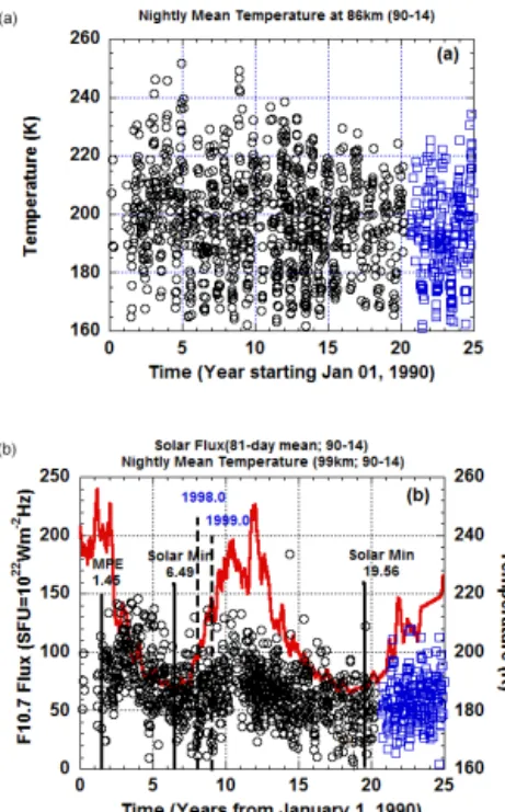
As an overview, we plot the 25 years of nightly mean tem-peratures at 86 km, which shows large annual and semian-nual variation, and at 99 km, an altitude with minimal ansemian-nual and small semiannual variation (She and von Zahn, 1998), respectively, in Fig. 1a and b. The data acquired at CSU (March 1990–March 2010) is in black and that acquired at USU (September 2010–December 2014) is in blue; apart from a small data gap in 2010, the two sets of data blend nicely. From Fig. 1a summer is about 60–80 K cooler than winter at 86 km. At 99 km one can see long-term tempera-ture variation. The 81-day averaged daily F10.7 solar flux also plotted in the figure, in the red curve, shows that the nightly mean temperatures track the variation in solar flux after 1993. Note that there exists a warming episode after the Mt Pinatubo Eruption (MPE), tMPE=1.45 years, which
peaked in 1993 and mostly died away near the beginning of 1999 for altitudes between 88 and 102 km (Fig. 3a). Since the warming episode is in our data, we must account for it in the analysis, whether its causes are fully understood or not. As a result, a nonlinear least-square regression analysis is required for long-term study.
Following She et al. (2009), who performed regression analysis on a shorter data set (90-07), a time series with 894 points, we express the nocturnal temperature at each al-titude,T (z, t ), of (90-14_Avg), a time series of 1200 points, as
T (z, t )=Tfit(z, t )+TRes(z, t ), (1)
where,
Figure 1.Time series of nocturnal mean temperature recorded by
a Na lidar at 86 km(a)and at 99 km (b). Included in(b)is also
81-day F10.7 solar flux in red with the times for Mount Pinatubo
eruption (MPE),tMPE, and solar minima (Solar Min) marked. Data
(black circles) between March 1990 and March 2010 were
ac-quired at CSU (41◦N, 105◦W), and those (blue circles) between
September 2010 and December 2014 were acquired at USU (42◦N,
112◦W).
Tfit(z, t )=α(z)+A1(z)cos(2π t )
+B1(z)sin(2π t )+A2(z)cos(4π t )
+B2(z)sin(4π t )+β(z)t+γ (z)P (z, t )
+δ(z)Q81(t );P (z, t )=2/{exp(t0−t ) /t1
+exp(t−t0) /t2},
where t is time in years from 1 January 1990, α(z) is independent of time, and the 4 A–B terms represent an-nual and semianan-nual variations. The three long-term ef-fects have the amplitudes β(z), γ (z), and δ(z), in this model. The strong warming episode in our data, initially attributed to the Mt Pinatubo eruption in June 1991 (She et al., 1998), is represented by an amplitude γ (z) times
P (z, t )=2/{exp(t0−t )/t1+exp(t−t0)/t2}, with
parame-ters t0(z), t1(z), and t2(z), for the delay, rise, and decay
time, respectively. The delay time here is relative to 1 Jan-uary 1990, with the Mt Pinatubo eruption at 1.45 years (see Fig. 1b). Other long-term responses includeδ(z), the solar response in K/SFU withQ81(t )being the 81-day averaged
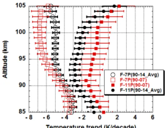
Figure 2.Linear temperature trend from the quarter century data set with 11- and 7-parameter analyses, respectively denoted as F-11P(90-14_Avg) in black solid circles and F-7P(90-14_Avg) in black open circles. Shown for comparison are those data published based on an 18-year data set denoted as F-11P(90-07) in red solid squares and F-7P(90-07) in open red squares.
Since all effects of comparable strengths must be included in the time series for the nonlinear regression analysis (Ak-maev, 2012) and the warming episode, solar activity and lin-ear trend are not independent, the best fit of one term will affect that of the other and they will depend upon the length of the data set.
3 Temperature trend deduced from quarter century lidar data
The long-term linear trend of the 11-parameter fit to the long data set, F-11P(90-14_Avg), is shown in Fig. 2 along with F-7P(90-14_Avg), deduced from the 7-parameter fit by set-tingγ (z)=0. Also shown are the published results from F-11P(90-07) and F-7P(90-07) from the shorter data set from March 1990 to 2007. As expected, the uncertainty from the 25-year data set is smaller than that from the 18-year data set. The cooling trend in F-11P(90-14_Avg) starts from an insignificant value of 0.64±0.99 K decade−1 at 85 km, in-creases to a maximum of 2.8±0.58 K decade−1between 91 and 93 km, and then gradually decreases to a warming trend above 103 km. Turning from a cooling to a warming trend above 100 to 120 km in geographic altitudes is the result of the cooling and contraction of underlying atmosphere, the lower thermosphere, the mesosphere, and the stratosphere; it is predicted by models (Akmaev, 2012; Qian et al., 2013). This does not occur in the seven-parameter analysis (see 7P(90-14_Avg) in Fig. 2). A similar difference between F-11P(90-07) and F-7P(90-07) is also evident. To our knowl-edge, metal resonance lidar is the only ground-based instru-ment that covers the entire mesopause region, and ours is the only Na lidar with a long enough data set to see this trend reversal.
Compared to the trends deduced from the shorter data set, (90-07), we note that the difference between F-7P(90-07) and F-11P(90-07) is bigger than the difference between F-7P(90-14_Avg) and F-11P(90-F-7P(90-14_Avg) because the influence of the warming episode on the temperature trend is reduced in a longer data set. Statistically, the results from the longer data set are more accurate; the mean uncertainty between 88 and 102 km is 0.6 and 1.3 K decade−1, respectively, for 14_Avg) and the previously published F-11P(90-07). However, below we investigate the discrepancy between the two 11-parameter analyses, i.e., the 25-year data set has a larger cooling trend by∼1 K decade−1.
Since the three long-term effects with magnitudes
β(z), γ (z), andδ(z)are not independent in our analysis, we can understand their mutual influences by realizing that, in addition to the annual and semiannual variations, the ob-served temperature at a given time is the sum of three con-tributionsβ(z)t, γ (z)P (z, t ), and δ(z)Q81(t ). Because the
solar flux,Q81(t ), is a quasi-periodic function with a period
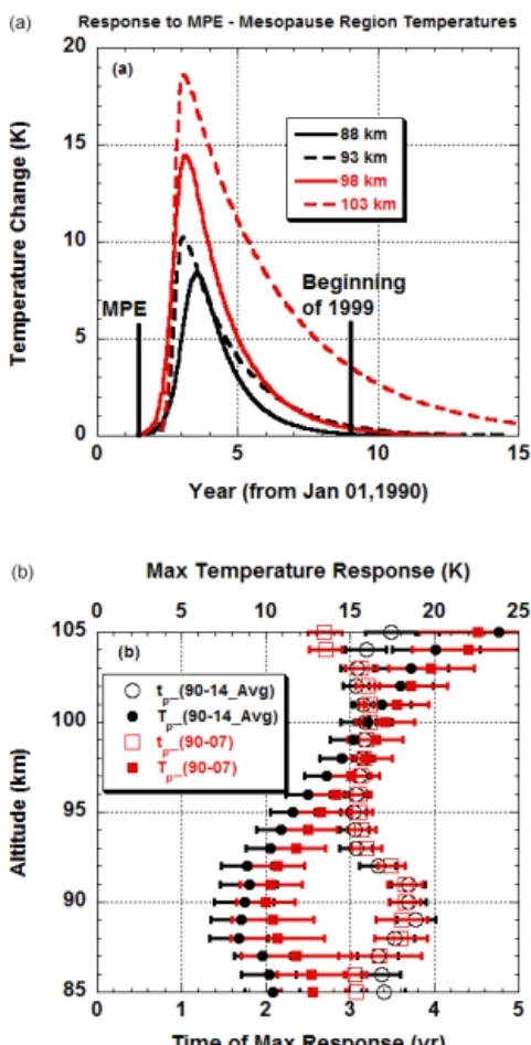
of∼11 years, for data sets longer than 11 years, the dominat-ing competition is between the warmdominat-ing episode and trend. There is then a trade-off between the two best-fit values, which depend upon the observed values in the entire time series, i.e., data length. To see how this interdependence or correlation affects the∼1 K decade−1discrepancy more ex-plicitly, we recall that the proxy of the warming episode is the functionγ (z)P (z, t ), which is shown in Fig. 3a for selected altitudes. This function rises to a peak temperature (max tem-perature),Tp, at the timetp=t0+ℓn(t2/t1)/[(1/t1)+(1/t2)]. Comparingtp andTpin the 25- and 18-year-long data sets reveals the difference of their warming episode affecting the temperature trend. We plot these quantities as a function of altitude in Fig. 3b for 14_Avg) and for F-11P(90-07). Note that the altitude dependences for the two data sets are similar. Between 88 and 102 km, where the lidar signal is strong, we see little difference intpbut a systematic
dif-ference inTpbetween the two data sets. Above 93 km,tpis
about constant, butTpincreases continuously. Note that the
peak warming (or maximum temperature response),Tp, from
Figure 3. (a)Episodic warming in the 1990s at selected altitudes. By the beginning of 1999, the warming episode is basically over
between 88 and 102 km.(b)The peak temperature (maximum
tem-perature response),Tp, and the time at which it occurs (or the time of
max response),tp, of warming episode deduced from 25-year data
set (90-14_Avg) is shown in black solid circles and open circles, respectively. Results shown in red solid squares and open squares were deduced from the 18-year data set (90-07).
4 Discussions
The warming episode in our data plays a critical role in the temperature trend analysis based on our data sets. Further-more, we assume a single temperature trend over 25 years in analysis. We thus shall discuss these issues before the final conclusion.
4.1 Mesopause warming and global surface cooling in the 1990s
A significant 6 K warming in 1992 and 1993 between 60 and 80 km was reported by Rayleigh lidar observations in southern France and attributed to the Mt Pinatubo eruption (Keckhut et al., 1995). Our suggestion (She et al., 1998) that the observed warming episode is one of the consequences of the Mt Pinatubo eruption does not yet have a clear geophysi-cal causal relationship. To our knowledge, there has been no succinct explanation or model simulation published that
re-lates the direct radiative and/or indirect dynamical effects of the Pinatubo eruption to the observed response in the meso-sphere which lingered for∼7 years at altitudes between 88 and 102 km as shown in Fig. 3a. There is, however, a compre-hensive study of global mean surface temperature change in response to volcanic eruption and ENSO (El Niño–Southern Oscillation) events by Thompson et al. (2009). In response to the Mt Pinatubo eruption, they found a peak cooling of ∼0.3 K about 1.5 years after the Pinatubo eruption, which, remarkably, also lingered for∼7 years. Changing the sign of their deduced global surface temperature response and mul-tiplying it by a factor of 50, we obtain an episodic response very similar to our mesopause region temperatures response. Better yet, we find that the scaled global surface temperature change, STR·(−50), deduced by Thompson et al. (2009) can be fitted to γ (z)P (z, t )that was used to represent the warming episode deduced from Na lidar observation. Next, we compare the peak delay time and the response time con-stant,tpd=tp−tMPE=tp−1.45, andτ=t1+t2, respectively,
for the two observed episodes that occurred in the same time frame but∼100 km apart in height.
Thompson et al. (2009) analyzed the surface tempera-ture response to a volcanoT (t )by using the forcing func-tion F (t ) in terms of a simple model system of exponen-tial decaying memory with time constant τ0=Cβ, where C is the effective heat capacity of the global atmospheric– oceanic mixed layer per unit area andβis the damping coeffi-cient, a measure of the climate sensitivity. They deducedC= 4.8×10⁷J m−2K−1, equivalent to the effect of the global at-mosphere plus 9 m of the global oceanic mixed layer, and set
β to be 2/3 K (W m−2)−1leading to a time constant for the
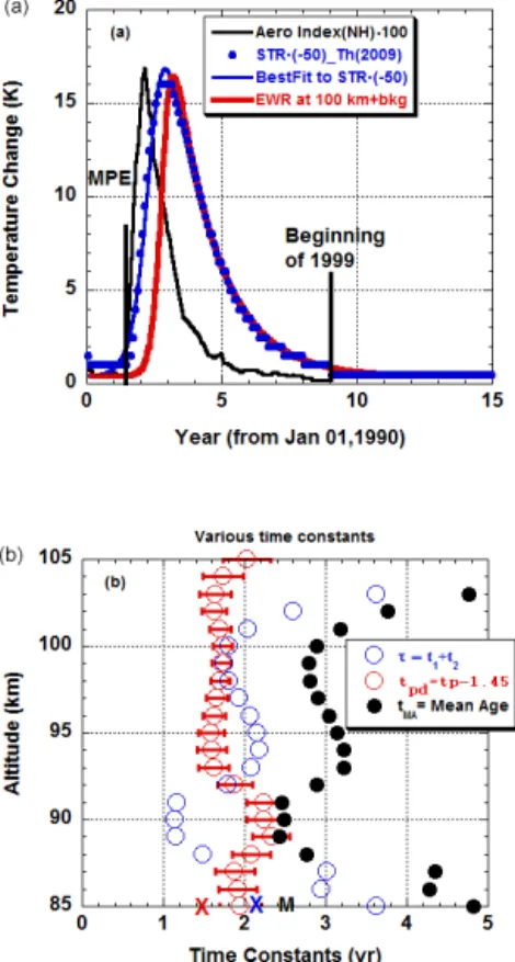
model system ofτ0=Cβ=3.2×10⁷s=1.01 years. Though the system response to an impulse is a simple exponential decaying function with a memory of ∼1 year, the forc-ing function, with the Northern Hemisphere aerosol index as a proxy lasted several years through the end of 1994. The Aero Index (NH)·100 is shown in Fig. 4a. Thomp-son et al. (2009) produced a cumulative response with a memory much longer than 1 year; the scaled response, STR·(−50), is also shown. Since STR·(−50) has a shape similar to the mesopause region warming episode, we fit it to the functionγ (0)P (0, t )+background, givingγ =13.0 K,
t0=2.42 years, t1=0.35 years, t2=1.70 years, and tp= 2.88 years, along with a background of 0.39 K, shown in Fig. 4a as the blue curve, which is seen to match the scaled surface temperature response very well. The time constant and peak delay time for the global surface temperature re-sponse are, respectively,τ =2.05 years andtpd=1.43 years.
Also in Fig. 4a is the warming response at 100 km in altitude (with the same background of 0.39 K added), the best-fit pa-rameters of which areγ =11.4 K,t0=2.81,t1=0.20 years, t2=1.60 years and tp=3.17 years, orτ =1.80 years and tpd=1.65 years. It is evident that both blue and red curves
Figure 4. (a) A comparison between 100·stratospheric aerosol (black) and the scaled global surface temperature response,
STR·(−50), in blue dots, from Thompson et al. (2009), along
with its best fit (blue curve) and episodic warming response (EWR) in temperatures at 100 km (red curve). Both STR and
EWR are over at the beginning of 1999, ∼7.5 years after the
Mt Pinatubo eruption. (b) Deduced altitude-dependent time
con-stant of the response,τ, peak delay time,tpd, and mean age,tMA,
for the warming episodic function, respectively in open blue cir-cles, open red circir-cles, and solid black circles. Marked at the bot-tom of the figure are the times for the surface temperature re-sponse, respectively by blue and red crosses and the letter M. Data,
STR·(−50) in(a)is derived from http://www.atmos.colostate.edu/
~davet/ThompsonWallaceJonesKennedy/.
A more complete comparison between the warming episode in the mesopause region temperatures and the global surface temperature anomaly is shown in Fig. 4b, where the warming episode response time constantτ and peak de-lay timetpd are plotted as a function of altitude along with these values for the surface temperature response at the bot-tom of the figure. Averaged over the warming episode be-tween 88 and 102 km, we find τ =1.81±0.42 years and
tpd=1.82±0.26 years, compared with the surface
temper-ature anomaly ofτ =2.05 years andtpd=1.43 years. In
ad-dition, since the functional shape of both anomalies repre-sents the distribution of the transit times of respective events, the concept of the “age of air” (AOA) (Waugh and Hall, 2002) is useful. Though the AOA concept was mostly ap-plied to the transport of species from the tropical troposphere
to the stratosphere, we use it here to describe the temporal history of an episodic response to a strong impulsive forc-ing. In fact, when area is normalized, the response of both surface temperature and mesopause temperatures after the Mt Pinatubo eruption is what is called the “age spectrum” in the AOA literature. Though all information on the trans-port process in question is contained in the age spectrum, the mean age (or the first moment of the spectrum in refer-ence to the time of the forcing impulse, i.e.,tMPEhere) of air, tMA, may be used as a rough measure of the life of the
pro-cess. With the “age spectrum” at each altitude, we can com-pute the associated mean age,tMA, also plotted in the figure, along with an upper-case M for the surface temperature re-sponse,tMA=2.51 years. Averaged between 88 and 102 km, we havetMA=2.92±0.33 years for the warming response.
All these time constants are deduced from observational data. Assuming the Pinatubo aerosol reached the tropical lower stratosphere in negligible time as Mt Pinatubo erupted, for the warming episode, the mean agetMA is the time that
the direct plus indirect (dynamic and feedback) effect of Pinatubo aerosol reaches the midlatitude mesopause region from the tropic lower stratosphere. For global surface cool-ing, the timetMA starts as the perturbation moves from the
tropical lower stratosphere down through the global tropo-sphere to the global atmospheric–oceanic mixed layer and the subsurface ocean (Thompson et al., 2009). We propose no detailed mechanism, which may be complicated, that leads to the mesopause warming after the Mt Pinatubo erup-tion. We hope that similarities in the observed and deduced response times between the volcanic eruption and the ob-served episodes, along with treating the surface temperature cooling with the same response function, will spur scien-tists and modelers to ascertain the causal effects of these strong episodic responses that occurred at the same time but ∼100 km apart in height.
4.2 A single linear trend or piecewise linear trends
The use of a single linear trend for a long data set is con-sistent with the classic recommendation of the World Mete-orological Organization (WMO), using∼30 years or more for analysis (Cnossen, 2012), and the practice of modelers, typically using 20 or∼50 years of simulation for trend stud-ies (Akmaev et al., 2006; Garcia et al., 2007; Berger and Lübken, 2011). It is nonetheless an assumption (Laštoviˇcka et al., 2012). Since a primary cause of a long-term temper-ature change is the anthropogenic emission of greenhouse gases, a single linear trend over a 25-year span may not re-flect the reality of the rate of greenhouse emission changes. The emission of CO2and CH4into the atmosphere continues
to increase. Indeed, Emmert et al. (2012) recently reported the observed increase of thermospheric CO2concentration.
2011). In the midlatitudes, the trend began to reverse in the late 1990s (Akmaev, 2012; Qian et al., 2013), and it has been stabilized in recent years at a level below that in the 1960s. This recent O3rate change should slow down the cooling rate
in the mesosphere and justify the use of a nonlinear (Keck-hut et al., 2011) or piecewise linear trend for the regression analysis (Laštoviˇcka et al., 2012). Indeed, in analyzing the long-term variation in the reflection heights of radio waves from 1961 to 2009 (Bremer and Berger, 2002) and investi-gating temperature trends in the summer mesopause, Berger and Lübken (2011) and Lübken et al. (2013) found it ap-propriate to use three different linear trends with breaking points in 1979 and 1997. One could then reanalyze our 25-year data using piecewise trends in the future. In this case, we would replace the term β(z)t in Eq. (1) by two differ-ent linear trends joined at a breaking point. Again, because the influences of solar flux, warming episode, and trends on temperatures are not independent, all these terms, along with the break point, if it is to be statistically determined, must be included in Eq. (1) to compete for the same nightly mean temperatures for regression analysis.
5 Conclusions
We have performed a regression analysis for the deduc-tion of the mesopause region temperature trend based on an unprecedented Na lidar data set between March 1990 and December 2014. The 81-day averaged F10.7 solar is used as a proxy for solar activity, and a linear trend is as-sumed. Owing to a strong warming episode in the 1990s, the quarter century data set (90-14_Avg) is least-square fit-ted to an 11-parameter nonlinear model. The temperature trend shown in Fig. 2 starts from an insignificant value of 0.64±0.99 K decade−1 at 85 km, increases to a maxi-mum of 2.8±0.58 K decade−1between 91 and 93 km, and then gradually decreases to a warming trend above 103 km. Compared to the trend from the shorter data set, (90-07), which has a marginally significant cooling maximum of 1.55±1.15 K decade−1at 91 km (She et al., 2009), the quar-ter century data set gives a statistically quite significant cool-ing trend, larger by∼1 K decade−1. The discrepancy is due to the competition between warming episode and temper-ature trend. Since the longer data set assesses the long-lasting warming episode more fully, it leads to more signifi-cant results. The mean uncertainty between 88 and 102 km are 0.6 and 1.3 K decade−1, respectively, for the long and shorter data sets. The altitude dependence from the two data sets is quite similar, and their magnitudes are in the gen-eral range predicted by models. The trends reported here are −1.0±1.0 K decade−1at 87 km and−2.5±0.5 K decade−1 at 90 km; they are consistent with the recently reported trends: respectively, −2.3±0.6 K decade−1 (Offermann et al., 2010) and−4±2 K decade−1(Hall et al., 2012).
With regard to an interesting connection, we analyzed the surface temperature response after the Mt Pinatubo eruption reported by Thompson et al. (2009) with the same functional dependence as that used for the observed warming episode in the mesopause region. We determined the respective peak de-lay time,tpd, and mean age,tMA, to be, respectively, 1.43 and
2.51 years for surface temperature and 1.82 and 2.92 years for mesopause region warming. These similarities between the global surface temperature anomaly and the mesopause warming episode should hopefully spur community scien-tists and modelers to figure out the causal effects of these interesting phenomena.
Acknowledgements. The lead author expresses his appreciation to Rashi Akmaev, Rolando Garcia, Gary Thomas, Susan Solomon, Liying Qian, Uwe Berger, and Ingrid Cnossen for helpful discus-sion and offprints and to Dave Thompson for the use of surface temperature data. This study was performed as part of a collabo-rative research program supported under the Consortium of Reso-nance and Rayleigh Lidars (CRRL), National Science Foundation grants AGS-1041571, AGS-1135882, and AGS-1136082.
Topical Editor C. Jacobi thanks one anonymous referee for his/her help in evaluating this paper.
References
Akmaev, R. A.: On estimation and attribution of long-term temper-ature trends in the thermosphere, J. Geophys. Res., 117, A09321, doi:10.1029/2012JA018058, 2012.
Akmaev, R. A., Fomichev, V. I., and Zhu, X.: Impact of middle-atmospheric composition changes on greenhouse cooling in the upper atmosphere, J. Atmos. Sol.-Terr. Phy., 68, 1879–1889, 2006.
Beig, G.: Trends in the mesopause region temperature and our present understanding – an update, Phys. Chem. Earth, 31, 3–9, 2006.
Berger, U. and Lübken, F.-J.: Mesospheric temperature trends at midlatitudes in summer, Geophys. Res. Lett., 38, L22804, doi:10.1029/2011GL049528, 2011.
Bremer, J. and Berger, U.: Mesospheric temperature trends derived from ground-based LF phase-height observations at middle lati-tudes: Comparison with model simulations, J. Atmos. Sol.-Terr. Phys., 64, 805–816, 2002.
Cnossen, I.: Climate Change in the upper atmosphere,
Chap. 15, Greenhouse Gases – Emission, Measurement and Mangement, edited by: Liu, G., ISBN
978-953-51-0323-3, available at: http://www.intechopen.com/books/
greenhouse-gases-emission-measurement-and-management/ climate-change-in-the-upper-atmosphere, 2012.
Hall, C. M., Dyrland, M. E., Tsutsumi, M., and Mulligan, F. J.: Temperature trends at 90 km over Svalbard, Norway (78N, 16 E), seen in one decade of meteor radar observations, J. Geophys. Res., 117, D08104, doi:10.1029/2011JD017028, 2012.
Hassler, B., Daniel, J. S., Johnson, B. J., Solomon, S., and Olt-mans, S. J.: An assessment of changing ozone loss rates at South Pole: Twenty-five years of ozonesonde measurements, J. Geo-phys. Res., 116, D22301, doi:10.1029/2011JD016353, 2011. Keckhut, P., Hauchecorne, A., and Chanin, M. L.: Midlatitude
long-term variability of the middle atmosphere: trends and cyclic and episodic changes. J. Geophys. Res., 100, 18887–18897, 1995. Keckhut, P., Randel, W. J., Claud, C., Leblanc, T., Steinbrecht,
W., Funatsu, B. M., Bencherif, B. M., McDermid, I. S., Hauchecorne, A., Long, L., Lin, R., and Baumgarten, G.: An evaluation of uncertainties in monitoring middle atmosphere temperatures with the ground-based lidar network in support of space observations, J. Atmos. Sol.-Terr. Phy., 73, 627–642, doi:10.1016/j.jastp.2011.01.003, 2011.
Lašttoviˇcka, J., Solomon, S. C., and Qian, L.: Trend in the neutral and ionized upper atmosphere, Space Sci. Rev., 168, 113–145, doi:10.1007/s11214-011-9799-3, 2012.
Lübken, F.-J., Berger, U., and Baumgarten, G.: Temperature trends in the midlatitude summer mesosphere, J. Geophys. Res. Atmos., 118, 13347–13360, doi:10.1002/2013JD020576, 2013.
Offermann, D., Hoffmann, P., Knieling, P., Koppmann, R., Ober-heide, J., and Steinbrecht, W.: Long-term trends and solar cy-cle variations of mesospheric temperature and dynamics, J. Geo-phys. Res., 115, D18127, doi:10.1029/2009JD013363, 2010. Qian, L., Marsh, D., Merkel, A., Solomon, S. C., and Roble, R.
G.: Effect of trends of middle atmosphere gases on the meso-sphere and thermomeso-sphere, J. Geophys. Res.-Space, 118, 3846– 3855, doi:10.1002/jgra.50354, 2013.
Roble, R. G. and Dickinson, R. E.: How will changes in carbon dioxide and methane modify the mean structure of the meso-sphere and thermomeso-sphere?, Geophys. Res. Lett., 16, 1441–1444, 1989.
Schmidt, H., Brasseur, G. P., Charron, M., Manzini, E., Giorgetta, M. A., Diehl, T., Fomichev, V. I., Kinnison, D., Marsh, D., and Walters, S.: The HAMMONIA Chemistry Climate Model: Sen-sitivity of the Mesopause Region to the 11-year Solar Cycle and
CO2Doubling, J. Climate, 19, 3903–3931, 2006.
She, C. Y. and von Zahn, U.: The concept of two-level mesopause: Support through new lidar observation, J. Geophys. Res., 103, 5855–5863, 1998.
She, C. Y., Thiel, S. W., and Krueger, D. A.: Observed episodic warming at 86 and 100 km between 1990 and 1997: Effects of Mount Pinatubo eruption, Geophys. Res. Lett., 25, 497–500, 1998.
She, C.-Y., Krueger, D. A., Akmaev, R., Schmidt, H., and Talaat, E., and Yee, S.: Long-term variability in mesopause region
tem-peratures over Fort Collins, CO (41◦N, 105◦W) based on lidar
observations from 1990 through 2007, J. Atmos. and Sol.-Terr. Phy., 71, 1558–1564, doi:10.1016/j.jastp.2009.05.007, 2009. Thompson, D. W. J., Wallace, J. M., Jones, P. D., and Kennedy, J. J.:
Identifying signatures of natural climate variability in time series of global-mean surface temperature: Methodology and Insights, J. Climate, 22, 6120–6142, 2009.