BGD
12, 14941–14980, 2015
Interannual variability of the Mediterranean
trophic regimes
N. Mayot et al.
Title Page
Abstract Introduction
Conclusions References
Tables Figures
◭ ◮
◭ ◮
Back Close
Full Screen / Esc
Printer-friendly Version Interactive Discussion
Discussion
P
a
per
|
Discussion
P
a
per
|
Discussion
P
a
per
|
Discussion
P
a
per
Biogeosciences Discuss., 12, 14941–14980, 2015 www.biogeosciences-discuss.net/12/14941/2015/ doi:10.5194/bgd-12-14941-2015
© Author(s) 2015. CC Attribution 3.0 License.
This discussion paper is/has been under review for the journal Biogeosciences (BG). Please refer to the corresponding final paper in BG if available.
Interannual variability of the
Mediterranean trophic regimes from
ocean color satellites
N. Mayot1, F. D’Ortenzio1, M. Ribera d’Alcalà2, H. Lavigne3, and H. Claustre1
1
Sorbonne Universités, UPMC Univ Paris 06, INSU-CNRS, Laboratoire d’Océanographie de Villefranche (LOV), 181 Chemin du Lazaret, 06230 Villefranche-sur-mer, France
2
Laboratorio di Oceanografia Biologica, Stazione Zoologica “A. Dohrn”, Villa Comunale, 80121 Napoli, Italy
3
Istituto Nazionale di Oceanografia e di Geofisica Sperimentale (OGS), Borgo Grotta Gigante 42/c, 34010 Sgonico, Trieste, Italy
Received: 27 July 2015 – Accepted: 24 August 2015 – Published: 9 September 2015
Correspondence to: N. Mayot ([email protected])
BGD
12, 14941–14980, 2015
Interannual variability of the Mediterranean
trophic regimes
N. Mayot et al.
Title Page
Abstract Introduction
Conclusions References
Tables Figures
◭ ◮
◭ ◮
Back Close
Full Screen / Esc
Printer-friendly Version Interactive Discussion
Discussion
P
a
per
|
Discussion
P
a
per
|
Discussion
P
a
per
|
Discussion
P
a
per
Abstract
D’Ortenzio and Ribera d’Alcalà (2009, DR09 hereafter) divided the Mediterranean Sea into “bioregions” based on the climatological seasonality (phenology) of phytoplank-ton. Here we investigate the interannual variability of this bioregionalization. Using 16 years of available ocean color observations (i.e. SeaWiFS and MODIS), we analyzed
5
the spatial distribution of the DR09 trophic regimes on an annual basis. Additionally, we identified new trophic regimes, with seasonal cycles of phytoplankton biomass dif-ferent from the DR09 climatological description and named “Anomalous”. Overall, the classification of the Mediterranean phytoplankton phenology proposed by DR09 (i.e. “No Bloom”, “Intermittently”, “Bloom” and “Coastal”), is confirmed to be representative
10
of most of the Mediterranean phytoplankton phenologies. The mean spatial distribution of these trophic regimes (i.e. bioregions) over the 16 years studied is also similar to the
one proposed by DR09. But at regional scale some annual differences, in their
spa-tial distribution and in the emergence of “Anomalous” trophic regimes, were observed compared to the DR09 description. These dissimilarities with the DR09 study were
re-15
lated to interannual variability in the sub-basin forcing: winter deep convection events,
frontal instabilities, inflow of Atlantic or Black Sea Waters and river run-off. The large
assortment of phytoplankton phenologies identified in the Mediterranean Sea is thus verified at interannual level, confirming the “sentinel” role of this basin to detect the impact of climate changes on the pelagic environment.
20
1 Introduction
The Mediterranean Sea is one of the oceanic regions the most impacted by climate change (Giorgi, 2006; Giorgi and Lionello, 2008). These important environmental mod-ifications are supposed to strongly modify the dynamics of the Mediterranean marine ecosystems (The Mermex Group, 2011), by modifying the food web structure (Coll et
25
BGD
12, 14941–14980, 2015
Interannual variability of the Mediterranean
trophic regimes
N. Mayot et al.
Title Page
Abstract Introduction
Conclusions References
Tables Figures
◭ ◮
◭ ◮
Back Close
Full Screen / Esc
Printer-friendly Version Interactive Discussion
Discussion
P
a
per
|
Discussion
P
a
per
|
Discussion
P
a
per
|
Discussion
P
a
per
jellyfish blooms, Purcell, 2005), which should have strong consequences on human activities. In the climate change framework, phytoplankton plays a key role, because
any perturbations on its dynamic would affect the rest of the marine food web (Edwards
and Richarson, 2004). In a semi enclosed sea, relatively small, as is the Mediterranean, that kind of processes should be particularly accelerated. A modification of the
phyto-5
plankton communities could impact on the whole ecosystems much more rapidly than in other oceanic regions (Siokou-Frangou et al., 2010).
In the Mediterranean, as in many of the oceanic regions, the phytoplankton dy-namic is characterized by a strong spatio-temporal variability (Estrada, 1996; Mann and Lazier, 2006), determined by the concomitant influence of several biotic and
abi-10
otic factors (Williams and Follows, 2003; Mann and Lazier, 2006). The link between abi-otic factors and phytoplankton variability, in the Mediterranean Sea, has been mainly inferred by using satellite ocean color data (Antoine et al., 1995; Bosc et al., 2004; Mélin et al., 2011; Volpe et al., 2012). Based on band-ratio algorithms to infer surface
chlorophylla concentration (considered as a proxy of phytoplankton biomass), a
gen-15
eral picture of the Mediterranean was revealed, confirming and reinforcing what had been derived by the relatively scarce existing in situ estimations, e.g., the presence of a widespread oligotrophy, of strong east-west and north-south gradients, the coastal influences, and the occurrence of blooming episodes in well-defined regions.
However, despite the ecological relevance of phytoplankton seasonality (or
phenol-20
ogy), which provides a powerful tool to identify the factors affecting ecosystem
func-tion (Edwards and Richarson, 2004), phenology has been relatively under considered in the Mediterranean. Phytoplankton phenology was generally hard to evaluate, as available observations were not at the temporal and/or spatial resolution required (see review of Ji et al., 2010), or were restricted to coastal areas. Satellite observations
25
BGD
12, 14941–14980, 2015
Interannual variability of the Mediterranean
trophic regimes
N. Mayot et al.
Title Page
Abstract Introduction
Conclusions References
Tables Figures
◭ ◮
◭ ◮
Back Close
Full Screen / Esc
Printer-friendly Version Interactive Discussion
Discussion
P
a
per
|
Discussion
P
a
per
|
Discussion
P
a
per
|
Discussion
P
a
per
proposed (D’Ortenzio and Ribera d’Alcalà, 2009, DR09 thereafter). Although limited to the surface only, DR09 identified in the available SeaWiFS ocean color dataset, seven recurrent patterns in seasonal cycles of phytoplankton in the Mediterranean. The observed seasonal patterns (referred by DR09 as “trophic regimes”) were then regrouped in four main classes on the basis of their shape characteristics: a
“temper-5
ate seas-like” dynamic (referred by DR09 as “Bloom”, characterized by a spring peak), a “tropical seas-like” dynamic (referred by DR09 as “No bloom”, to indicate the ab-sence of a marked peak), an “intermittently” dynamic (considered as an intermediate regime between “Bloom” and “No Bloom” trophic regimes, and interpreted as an arti-factual regime produced by averaging) and a “Coastal” dynamic (frequently observed in
10
coastal regions, see later). Moreover, the geographical distribution of the DR09 trophic regimes followed well-defined spatial patterns, and was thus interpreted as a
biore-gionalization of the basin based on the phenological traits of the surface chlorophylla
concentration. Compared to existing Mediterranean bioregionalization (e.g. Nieblas et al., 2014), the DR09 approach is specifically focused on the seasonal cycles of
phyto-15
plankton and, consequently, is adapted to address issues of phytoplankton phenology. The DR09 results has been already used to investigate the role of the mixed layer depth (MLD) and of nitrate distribution on the Mediterranean phytoplankton phenology (Lavigne et al., 2013), while modeling studies have used the DR09 bioregionaliza-tion based on the seasonal dynamics of phytoplankton to ameliorate the primary
pro-20
duction estimates from space (Uitz et al., 2012). Combining temporal (i.e. the trophic regimes) and spatial (i.e. the bioregions) analysis, the DR09 results provided thus a robust framework to identify the role of abiotic and biotic factors on the Mediterranean phytoplankton phenology.
Two main issues are, however, still unresolved. Firstly, the DR09 results were
ob-25
chloro-BGD
12, 14941–14980, 2015
Interannual variability of the Mediterranean
trophic regimes
N. Mayot et al.
Title Page
Abstract Introduction
Conclusions References
Tables Figures
◭ ◮
◭ ◮
Back Close
Full Screen / Esc
Printer-friendly Version Interactive Discussion
Discussion
P
a
per
|
Discussion
P
a
per
|
Discussion
P
a
per
|
Discussion
P
a
per
phylla, could have generated unrealistic seasonal cycles of phytoplankton. This point,
already evoked by the authors, is particularly relevant for the “Intermittently” trophic regime of DR09 (see also the discussion on the “Intermittently” DR09 trophic regime in Lavigne et al., 2013).
In this paper, we reappraised the DR09 approach with the specific aim to take into
5
account the interannual variability of the Mediterranean surface chlorophylla
concen-tration. A new method is proposed to identify the relevance of the DR09 trophic regimes on an annual basis. The method identifies also the discrepancy from the DR09 climato-logical trophic regimes, by allowing the emergence of totally new (compared to DR09) patterns of seasonality (i.e. new trophic regimes) that could have been masked by the
10
climatological approach of DR09. The satellite database is also expanded, by including seven additional years of ocean color data compared to the DR09 paper. The discus-sion is focused on the interannual variability of the DR09 trophic regimes and on the occurrence of the new trophic regimes. A step forward in the interpretation of the trophic regimes is proposed (the DR09 ones and the new ones) by considering their frequency
15
of occurrence at basin and regional scales, simultaneously with forcing processes.
2 Data and methods
2.1 Data
Surface chlorophyll a concentration ([Chl]surf) from Level 3 images of SeaWiFS and
MODIS Aqua, at spatial and temporal resolution of respectively 8 days and 9 km,
20
were downloaded from the NASA’s OceanColor website (http://oceandata.sci.gsfc. nasa.gov/), for the period 1998-2014. SeaWiFS data were used for the period 1998– 2007, while MODIS Aqua data were used after July 2007. MODIS and SeaWiFS datasets were already shown to be consistent (Franz et al., 2005). The resulting
16-years satellite database was initially divided on a yearly basis (from July of yearT−1
25
BGD
12, 14941–14980, 2015
Interannual variability of the Mediterranean
trophic regimes
N. Mayot et al.
Title Page
Abstract Introduction
Conclusions References
Tables Figures
◭ ◮
◭ ◮
Back Close
Full Screen / Esc
Printer-friendly Version Interactive Discussion
Discussion
P
a
per
|
Discussion
P
a
per
|
Discussion
P
a
per
|
Discussion
P
a
per
In the Mediterranean Sea, an overestimation of the [Chl]surfretrieved from space was
identified by comparison with in-situ data (Gitelson et al., 1996; Claustre et al., 2002), particularly at the low values (e.g. Fig. 14 from Antoine et al., 2008). However, to keep the consistency with the DR09 analysis, the NASA standard products for SeaWiFS and MODIS (O’Reilly et al., 1998) are used here, instead of alternative products
gener-5
ated with regional algorithms. Consequently, as in DR09, to minimize the impact of the
[Chl]surf algorithms artifacts, each annual time series was normalized by its maximal
value. In what follows, the time series (from July to June) of a specific year are referred
as “annual” time series of normalized surface chlorophyllaconcentration (nChl).
2.2 Interrannual clustering
10
The method proposed here refines the DR09 method on an annual basis and then identifies new trophic regimes, which were hidden in the climatological DR09 approach. The method consists in identifying, for each “annual” time series of each pixel, the closest DR09 trophic regime having the most similar seasonal cycle. When a time
series is different, beyond a chosen threshold, from all DR09 trophic regimes, it is
15
initially considered apart, in a sub-set of the initial database. All the time series of this subset are finally clustered to define new trophic regimes.
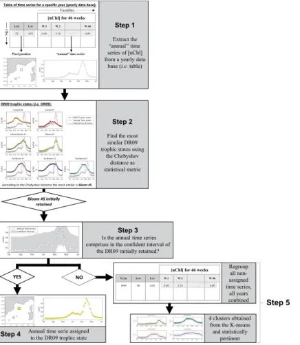
In practice (see Fig. 1):
1. for each year and for each Mediterranean pixel, the “annual” time series ofnChl
and its corresponding geographical position are extracted (Fig. 1, step 1).
20
2. The similarity between the “annual” time series and each of DR09 trophic regimes
is evaluated using the Chebytchev distance (defined as the greatest difference
between the time series and any DR09 trophic regimes). The DR09 trophic regime having the lowest distance with the “annual” time series is initially selected (Fig. 1, step 2).
BGD
12, 14941–14980, 2015
Interannual variability of the Mediterranean
trophic regimes
N. Mayot et al.
Title Page
Abstract Introduction
Conclusions References
Tables Figures
◭ ◮
◭ ◮
Back Close
Full Screen / Esc
Printer-friendly Version Interactive Discussion
Discussion
P
a
per
|
Discussion
P
a
per
|
Discussion
P
a
per
|
Discussion
P
a
per
3. To be definitively assigned to the selected DR09 trophic regime, the “annual” time series must be contained in the confidence interval of that DR09 trophic regime. The confidence interval is defined as the mean Chebyshev distance between the
DR09 trophic regime and all the weekly climatological time series of nChl used
by DR09 that belong to this trophic regime, plus 1.5 times the standard deviation
5
(Fig. 1, step 3). Note that the confidence interval is different for each DR09 trophic
regimes.
4. If the “annual” time series falls within the confidence interval, then the “annual” time series and its pixel are assigned to the DR09 trophic regime initially selected (Fig. 1, step 4). Otherwise, the “annual” time series (and its associated pixel) is
10
temporarily added to a table with all “non-assigned” time series.
5. All of the “non-assigned” time series (from of all the 16 years combined) were clustered using the same methodology as in DR09 (a K-means clustering, Har-tigan and Wong, 1979) (Fig. 1, step 5). The number of clusters is decided using the Calinski and Harabasz index (which is a criterion based on the ratio of the
15
within and between cluster variance, Calinski and Harabasz, 1974; Milligan and Cooper, 1985). Then, the stability of the resulting clusters was assessed by
com-paring them (using the Jaccard coefficient) with clustering results obtained after
a modification (i.e. adding an artificial noise), or a subset of the dataset (Hennig,
2007, see also DR09). Only clusters with a Jaccard coefficient greater than 0.75
20
are considered stable. These new clusters include all the “annual” time series that
are statistically different from the DR09 climatological time series. In some sense,
they represent anomalies compared to the DR09 climatological analysis and, for this reason, they are referred in the following as “Anomalous” trophic regimes.
Four “Anomalous” trophic regimes are obtained, and all are stable (i.e. presenting
Jac-25
card coefficients > 89 %). Overall, 77.2 % of the “annual” time series are classified
BGD
12, 14941–14980, 2015
Interannual variability of the Mediterranean
trophic regimes
N. Mayot et al.
Title Page
Abstract Introduction
Conclusions References
Tables Figures
◭ ◮
◭ ◮
Back Close
Full Screen / Esc
Printer-friendly Version Interactive Discussion
Discussion
P
a
per
|
Discussion
P
a
per
|
Discussion
P
a
per
|
Discussion
P
a
per
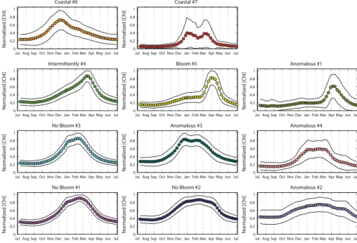
3 Results
The method described in Sect. 2.2 provides 11 time series (i.e. the seven DR09 trophic regimes and the four “Anomalous”) obtained by averaging all the “annual” time series
ofnChl based on their membership in one of the 11 trophic regimes (Fig. 2), as well as
16 annual maps of the spatial distribution of the 11 trophic regimes (Fig. 3). Following
5
the interpretation of DR09, we considered the spatial distribution of the trophic regimes as a bioregionalization, and we will refer the regions having the same trophic regime as a “bioregion”.
The main traits of the trophic regime time series will be sketched in the next para-graphs (for the seven DR09 and the four “Anomalous”), whereas their associated
geo-10
graphical distributions will be analyzed afterwards.
3.1 General patterns of DR09 trophic regimes
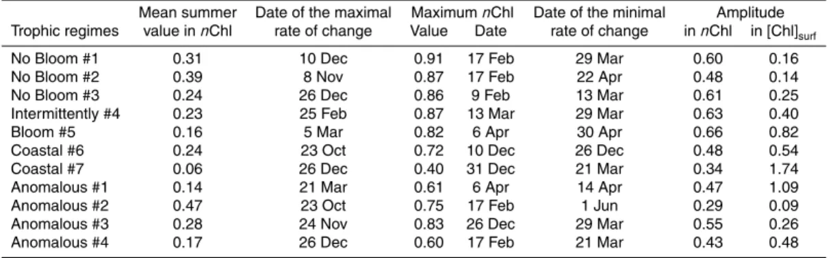
The nChl time series of the non-coastal DR09 trophic regimes (Fig. 2), despite their
common characteristics (they all present minimal value in summer, Table 1), display
different amplitudes ofnChl and of [Chl]surf (i.e. defined as the difference between the
15
mean summer value and the annual maximum values of nChl and [Chl]surf, Table 1).
The “Bloom #5” and “Intermittently #4” trophic regimes show the greatest amplitudes
(0.66nChl and 0.82 mg m−3 for “Bloom #5”, 0.63nChl and 0.40 mg m−3 for the
“In-termittently #4”), whereas the “No Bloom #2” trophic regime the lowest (0.48nChl and
0.14 mg m−3). The timings of the main events are also different. The dates of the annual
20
maximum values are observed in winter (in February) for “No Bloom” trophic regimes (#1, #2 and #3) and in spring for the “Intermittently #4” (13 March) and the “Bloom #5” (6 April) trophic regimes. The dates of the maximal rate of change (i.e. the date
of the highest first derivative of thenChl time series) are also increasing from the “No
Bloom”, the “Intermittently #4”, to the “Bloom #5”, whereas the dates of the minimum
25
rate of change (i.e. the date of the lowest first derivative of thenChl time series) range
BGD
12, 14941–14980, 2015
Interannual variability of the Mediterranean
trophic regimes
N. Mayot et al.
Title Page
Abstract Introduction
Conclusions References
Tables Figures
◭ ◮
◭ ◮
Back Close
Full Screen / Esc
Printer-friendly Version Interactive Discussion
Discussion
P
a
per
|
Discussion
P
a
per
|
Discussion
P
a
per
|
Discussion
P
a
per
The “Coastal” DR09 trophic regimes show different seasonal characteristics from the
rest of the DR09 trophic regimes (Table 1). The maximum value of the “Coastal #6” time
series is lower (0.72nChl) and arrives earlier (in December) than for the other DR09
trophic regimes. The “Coastal #7”, which shows a double peak during winter months, exhibits also a great dispersion around the mean, indicating that the resulting mean
5
seasonal cycle is probably an artifact.
3.2 General patterns of the “Anomalous” trophic regimes
All of the “Anomalous” trophic regimes (#1, #2, #3 and #4) show minimum values of
nChl in summer (0.14nChl for the “Anomalous #1”, 0.47nChl for the “Anomalous #2”,
0.28nChl for the “Anomalous #3 and 0.17nChl for the “Anomalous #4”). The
“Anoma-10
lous #1” trophic regime shows an evident spring peak (starting on 21 March, maximal on 6 April and decreasing on 14 April), whereas “Anomalous #2”, “#3” and “#4” display a winter plateau, with their maximal rate of change and maximal values obtained in late fall and winter respectively (23 October and 17 February for “#2”, 24 November and 26 December for “#3” and 26 December and 17 February for “#4”).
15
All the above suggests that the “Anomalous” trophic regimes could be considered as modified versions of the DR09 trophic regimes. The “Bloom #5” and the “Anomalous #1” trophic regimes have similar shape, showing both a spring peak (for both the date
of the maximal value is 6 April). Although they differ slightly for the dates of the maximal
and minimal rate of change (5 March and 30 April for “Bloom #5”, and 21 March and 14
20
April for the “Anomalous #1”), the “Anomalous #1” trophic regime appears as a more
peaked version of the “Bloom #5” trophic regime, with a higher amplitude in [Chl]surf
(0.82 mg m−3for the “Bloom #5” and 1.09 mg m−3for the “Anomalous #1”).
Similarly, the “No Bloom #2” and the “Anomalous #2” trophic regimes could be
as-sociated. They both display weak amplitudes of nChl and of [Chl]surf (0.48nChl and
25
0.14 mg m−3for the “No Bloom #2”, 0.29nChl and 0.09 mg m−3for the “Anomalous #2”,
BGD
12, 14941–14980, 2015
Interannual variability of the Mediterranean
trophic regimes
N. Mayot et al.
Title Page
Abstract Introduction
Conclusions References
Tables Figures
◭ ◮
◭ ◮
Back Close
Full Screen / Esc
Printer-friendly Version Interactive Discussion
Discussion
P
a
per
|
Discussion
P
a
per
|
Discussion
P
a
per
|
Discussion
P
a
per
the date of the minimal rate of change, which is delayed of one month for the “Anoma-lous #2” (1 June) compare to the “No Bloom #2” (22 April). The “Anoma“Anoma-lous #2” trophic regime appears then as a smoothed version of the “No Bloom #2” trophic regime,
where the winter-to-summer difference is low.
Finally, the “No Bloom #3” and the “Anomalous #3” and “#4” trophic regimes have
5
similar shapes and spatial repartition (see the next section). However, the “Anomalous
#3” trophic regime displays differences in the timing of the maximal rate of change and
of the maximal value (24 November and 26 December for the “Anomalous #3”, and 26 December and 9 February for the “No Bloom #3”), and the “Anomalous #4” trophic
regime presents a lower maximal value ofnChl (0.60nChl) than the “No Bloom #3”
10
trophic regime (0.86nChl), indicating a variability in the timing of the peak between
in-dividual time-series, but a higher amplitude of [Chl]surf(0.48 mg m
−3
for the “Anomalous #4” and 0.25 for the “No Bloom #3”).
The association of the “Anomalous” trophic regimes with the DR09 trophic regimes confirms the general partitions proposed by DR09 into “Bloom” and “No Bloom” trophic
15
regimes. The low occurrence of the “Anomalous” trophic regimes indicates also that their importance in the basin behavior is low. They possibly signify an accentuation or a diminishing of the factors influencing the phytoplankton phenology, although they should be likely considered as temporary perturbations of the general “Bloom”/”No Bloom” regimes. We will discuss on this later.
20
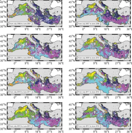
3.3 Geographical distribution of trophic regimes: interannual variability
The 16 annual maps, showing the spatial distribution of the 11 trophic regimes (Fig. 3), represent a first attempt to evaluate the interannual spatial variability of the bioregions (defined, in the sense of DR09, as regions having similar phytoplankton phenology or, more precisely, having the same trophic regime). In the next, the results are presented
25
sep-BGD
12, 14941–14980, 2015
Interannual variability of the Mediterranean
trophic regimes
N. Mayot et al.
Title Page
Abstract Introduction
Conclusions References
Tables Figures
◭ ◮
◭ ◮
Back Close
Full Screen / Esc
Printer-friendly Version Interactive Discussion
Discussion
P
a
per
|
Discussion
P
a
per
|
Discussion
P
a
per
|
Discussion
P
a
per
arately. The last paragraph will be dedicated to a wider analysis on the interannual spatio-temporal variability of the bioregions.
3.3.1 The “No Bloom” trophic regimes
Over the 16 years, “No Bloom” bioregions cover most of the Mediterranean surface (67.2 % on average, Fig. 4). The “No Bloom #1” is the most occurring “No Bloom”
5
bioregion over the 16 years analyzed (Fig. 4). Exceptions are observed in 1999, 2001, 2004, 2012 (dominance of the “No Bloom #3”) and in the 2000, 2007 (dominance of the “No Bloom #2”). The “No Bloom #1” bioregion is permanently observed in the Levantine basin and, often, in the Ionian Sea (Fig. 3). Episodically, it is also observed in the western basin, in particular over the Tyrrhenian Sea. During the 1999 to 2007
10
period, the “No Bloom #1” bioregion covered on average 25.6 % of the Mediterranean Sea, while from 2008 to 2014, its mean percentage increases to 33.5 %.
The second most occurring bioregion is the “No Bloom #3”, with a mean value of 21.5 % of covered surface over the 16 years (Fig. 4). It is associated with the Algerian basin (except in 2013 and 2014), although its northern and eastern boundaries are
15
more variable (Fig. 3). It is also observed in the North-Western Mediterranean (NWM), in the Tyrrhenian, and, sometimes (i.e. 2004 and 2012), in a large portion of the Eastern basin. No clear trends are observed over its interannual evolution, except that during the 1999, 2001, 2004 and 2012, it was the most extended bioregion.
Finally, the “No Bloom #2” bioregion covers on average 16.7 % of the Mediterranean
20
Sea (Fig. 4), and it is permanently observed in the Aegean and Adriatic Seas (Fig. 3). Peaks of occurrence are observed in the 2000 and 2007, when its distribution extended over the North Ionian (in 2000) and most of the Eastern Basin (in 2007). Similarly to the “No Bloom #1” bioregion, two periods could be identified in its interannual trend. Before 2008, the occurrence of the “No Bloom #2” bioregion is erratic, ranging from 11.5 to
25
BGD
12, 14941–14980, 2015
Interannual variability of the Mediterranean
trophic regimes
N. Mayot et al.
Title Page
Abstract Introduction
Conclusions References
Tables Figures
◭ ◮
◭ ◮
Back Close
Full Screen / Esc
Printer-friendly Version Interactive Discussion
Discussion
P
a
per
|
Discussion
P
a
per
|
Discussion
P
a
per
|
Discussion
P
a
per
3.3.2 The “Bloom” trophic regime
The “Bloom #5” bioregion covers on average 4 % of the Mediterranean Sea surface (Fig. 4), and it is observed quite exclusively in the NWM (Fig. 3). Notable exceptions are the years 1999 and 2006, when it is observed in the Southern Adriatic, and in 2003, in the Rhodes gyre area. The interannual variability of its extent (Fig. 4) ranges from very
5
low values (i.e. in 2001, 2007 and 2014) up to 9 % of the total Mediterranean surface (i.e. in 2005, which is, however, a special year due to high number of missing values). When the “Bloom #5” bioregion is weakly observed, it is generally replaced either by “Intermittently #4” (i.e. as in 2001 or in the 2007) or by the “Anomalous #1” bioregion (Fig. 3). In the first case, the “Intermittently #4” bioregion extends all over the NWM
10
with an almost total disappearance of the “Bloom #5” bioregion. In the second case, the “Bloom #5” bioregion is still present, but located in the border area of the NWM. The central area is instead occupied by the “Anomalous #1” bioregion (especially in 2005, 2006, 2008, 2010, 2013 and 2014).
3.3.3 The “Intermittently” trophic regime
15
On average, the “Intermittently #4” bioregion occupies 12.2 % of the Mediterranean sur-face (Fig. 4). This percentage is, however, strongly variable from one year to another, ranging from 7.2 % to almost 24.5 % of the total surface. It is permanently observed in the NWM, in the frontal area south of the large cyclonic gyre of the Ligurian Sea (Fig. 3). Its interannual variability is expressed by the high values of occurrence in 2003, 2006,
20
BGD
12, 14941–14980, 2015
Interannual variability of the Mediterranean
trophic regimes
N. Mayot et al.
Title Page
Abstract Introduction
Conclusions References
Tables Figures
◭ ◮
◭ ◮
Back Close
Full Screen / Esc
Printer-friendly Version Interactive Discussion
Discussion
P
a
per
|
Discussion
P
a
per
|
Discussion
P
a
per
|
Discussion
P
a
per
3.3.4 The “Coastal” trophic regimes
The “Coastal” bioregions cover on average 3.5 % of the Mediterranean (Fig. 4), with
a weak interannual variability (±1.5 %). The variability of the “Coastal” bioregions is
mainly driven by the variation of the occurrence of the “Coastal #6” bioregion, which represents 95 % of the “Coastal” bioregions occurrence. It is permanently observed in
5
the Gulf of Gabes and, more sporadically, in the west Adriatic coast (in 2002, 2003 and 2011, Fig. 3).
The “Coastal #7” bioregion presence is very low (less than 0.25 % of the Mediter-ranean surface), so we will neglect it in the next.
3.3.5 The “Anomalous” trophic regimes
10
The “Anomalous” bioregions occupy 12.8 % on average of the surface basin (Fig. 4), although they are primarily concentrated on coastal zones: the “Anomalous #2” biore-gion along the Adriatic and Aegean coasts, the “Anomalous #3” biorebiore-gion along the South Eastern basin coasts and the “Anomalous #4” bioregion along the Algerian coast (Fig. 3). Apart from coastal zones, the “Anomalous #1” bioregion is episodically
ob-15
served in the NWM, where it occupies a region usually classified as “Bloom #5” (see Sect. 3.3.2).
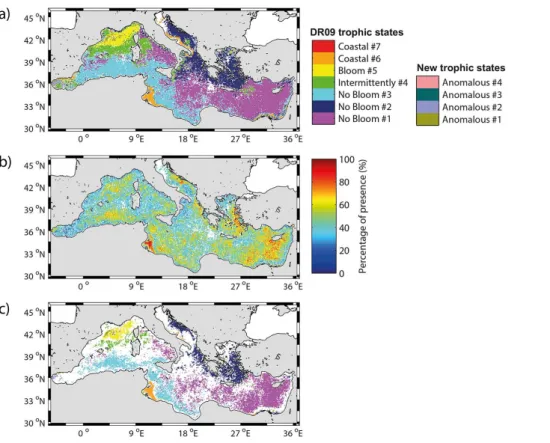
3.3.6 Dominance maps
Although the interannual variability of the geographical distribution of the bioregions is high, some general patterns emerge. To demonstrate this, a dominance map was
20
calculated by evaluating, for each pixel, the most recurrent bioregion (i.e. the domi-nant regime), over the 16 years period (Fig. 5a). Most of the Mediterranean basin is assigned to one of the DR09 bioregions (96 % of the map) and only 4 % to an “Anoma-lous” bioregion. A second map showing the degree of membership (defined as the percent of years in which each pixel belongs to its most recurrent bioregion, Fig. 5b)
BGD
12, 14941–14980, 2015
Interannual variability of the Mediterranean
trophic regimes
N. Mayot et al.
Title Page
Abstract Introduction
Conclusions References
Tables Figures
◭ ◮
◭ ◮
Back Close
Full Screen / Esc
Printer-friendly Version Interactive Discussion
Discussion
P
a
per
|
Discussion
P
a
per
|
Discussion
P
a
per
|
Discussion
P
a
per
was generated. The mean degree of membership over the whole Mediterranean area
is 46 % (Fig. 5b), quantifying the large interannual variability of the basin. Spatial diff
er-ences are, however, visible: coastal zones are generally characterized by low degree of memberships, while open ocean regions display higher values, showing less inter-annual variability.
5
To better highlight these geographical patterns, only areas with a degree of mem-bership greater than 50 % were plotted (Fig. 5c). The colored areas in Fig. 5c indicate where the bioregions are the most temporally recurrent, reflecting then the regions characterized by a weak interannual variability in the phenological traits. All the coastal areas (except in the Gulf of Gabes), as well as the regions at the frontier between
biore-10
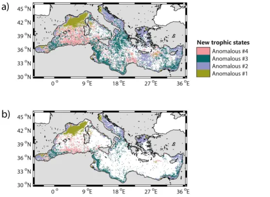
gions, disappear. Most of the “Intermittently #4” bioregion also disappear (maintained only in a limited region of the NWM), as well as, all the “Anomalous” bioregions (except the “Anomalous #1” bioregion in the NWM) and most of the region of the Alboran Sea. Similarly, a dominance map is generated considering only the four “Anomalous” bioregions (Fig. 6a), showing their patchy distribution and irregular occurrences.
How-15
ever, some spatial patterns exist, and are highlighted when only the pixels having at least two occurrences of the same “Anomalous” bioregion over the 16 years period were shown (Fig. 6b). The Anomalous #2, #3 and #4 bioregions are recurrently ob-served only all along the coasts. As always highlighted, the only open-ocean region exhibiting a coherent and recurrent “Anomalous” pattern is the NWM (classified as
20
“Anomalous #1”).
4 Discussion
4.1 Comparison with DR09 classification
The new method proposed here is intrinsically different from the DR09 one, although
it similarly provides trophic regimes and their spatial distributions (interpreted here as
BGD
12, 14941–14980, 2015
Interannual variability of the Mediterranean
trophic regimes
N. Mayot et al.
Title Page
Abstract Introduction
Conclusions References
Tables Figures
◭ ◮
◭ ◮
Back Close
Full Screen / Esc
Printer-friendly Version Interactive Discussion
Discussion
P
a
per
|
Discussion
P
a
per
|
Discussion
P
a
per
|
Discussion
P
a
per
bioregions). A comparison between the two approaches is therefore required before discussing the results.
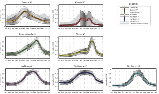
For this, we verified that the algorithms used in the new method provide the same results as the DR09 methodology (i.e. generation of a weekly climatological database and then application of a K-means clustering) when the results are presented in a
5
climatological point of view (i.e. in average over the 16 years). All the “annual” time
series of nChl were then averaged according to the DR09 trophic regimes to which
they belong (i.e. the DR09 trophic regimes time series in the Fig. 2), and compared to the DR09 evaluations (Fig. 7). The time series obtained with the new method are equivalent with the DR09 estimations: they are contained in the confidence interval
10
and they show similar standard deviations. The only notable discrepancy is observed for the “Coastal #7” trophic regime. Our interpretation is that the seasonal signal of this trophic regime (as obtained by DR09) is too ambiguous (i.e. high standard deviation, signal relatively flat) to be retrieved with the new method used here.
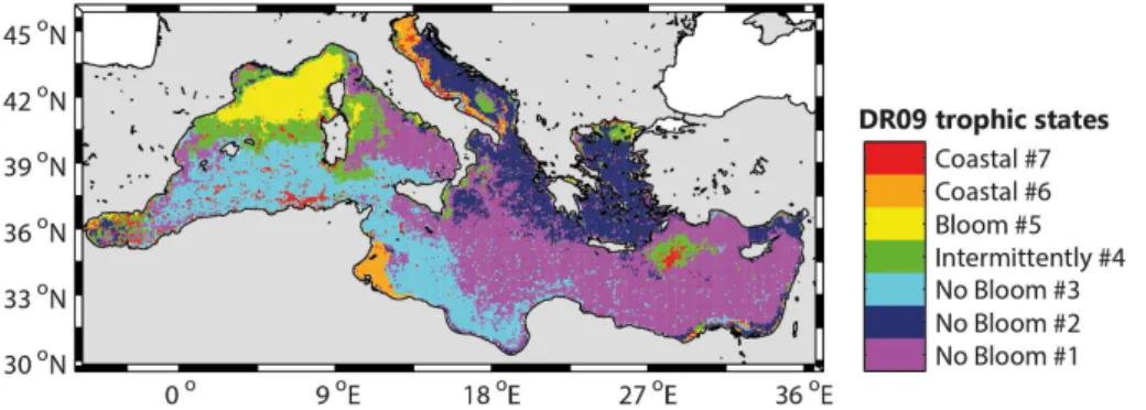
Furthermore, the spatial distribution of trophic regimes obtained with the DR09
15
methodology (Fig. 8) applied on the new 16-years database, is close to the domi-nance map of the Fig. 5a (74 % of similitude, defined as the percentage of pixels in the Fig. 5a belonging to the same DR09 trophic regime in the Fig. 8). However, some
differences with the DR09 10-years map (see Fig. 4 of DR09) exist, mainly the
dis-appearance of the “Intermittently #4” bioregion in the North Ionian. The differences
20
observed when using the new method could be then likely ascribed more to the natural interannual variability than to bias introduced by the new method. Note also that the
observed differences with the DR09 10-year map could additionally be ascribed to the
seven year extension of the database. In conclusion, the new method proposed here broadly supports the results of the DR09 analysis on the climatological timescale, but
25
there are some key differences generated by the larger extension of the database or
BGD
12, 14941–14980, 2015
Interannual variability of the Mediterranean
trophic regimes
N. Mayot et al.
Title Page
Abstract Introduction
Conclusions References
Tables Figures
◭ ◮
◭ ◮
Back Close
Full Screen / Esc
Printer-friendly Version Interactive Discussion
Discussion
P
a
per
|
Discussion
P
a
per
|
Discussion
P
a
per
|
Discussion
P
a
per
4.2 Interannual spatial variability of trophic regimes: significance and forcing
factors
The Fig. 5c clearly indicates that the interannual variability is for the most part con-centrated on the boundaries between the bioregions. In addition, the four “Anomalous”
trophic regimes, although statistically significant (i.e. Jaccard coefficient > 89 %), have
5
recurrent patterns in open-ocean only in the NWM (Fig. 6b). In the rest of the basin, they appear more as episodic fluctuations or noise than as real patterns. Although not surprising given the approach used (i.e. first finding occurrence of the DR09 trophic regimes and only second searching for anomalies), this point is not trivial. From the methodological point of view, the capability of the method to detect four anomalies
10
demonstrates its potential application in long-term studies. However, at a more in depth analysis and in view of an oceanographic interpretation, these anomalies are not partic-ularly relevant, as occurring only episodically and rarely indicating coherent, recurring patterns. Thus, the main climatological trophic regimes/bioregions identified by DR09
(i.e. “No Bloom”, “Bloom”, “Intermittently” and “Coastal”) are sufficiently comprehensive
15
to summarize the surface phytoplankton phenology in the Mediterranean Sea, even at interannual level. A notable exception in this global picture is the NWM area, with the recurrent occurrence of the “Anomalous #1” trophic regime.
Finally, it is important to note that, as suggested by DR09, trophic regimes (though
identified after normalization) are directly related to a specific range of [Chl]surf (see
20
Table 1). This point, confirmed here also for the “Anomalous” trophic regimes, suggests that the shape of the seasonal cycle is related to the stock of the phytoplankton biomass that the system could support. Based on the analysis of satellite surface data, this observation is certainly partial, although indicating a real pattern that merits further investigations.
BGD
12, 14941–14980, 2015
Interannual variability of the Mediterranean
trophic regimes
N. Mayot et al.
Title Page
Abstract Introduction
Conclusions References
Tables Figures
◭ ◮
◭ ◮
Back Close
Full Screen / Esc
Printer-friendly Version Interactive Discussion
Discussion
P
a
per
|
Discussion
P
a
per
|
Discussion
P
a
per
|
Discussion
P
a
per
4.2.1 The “No Bloom” trophic regimes
The bimodal pattern of “No Bloom” regimes, with a higher biomass in fall-winter and lower biomass in spring-summer, were explained in DR09 by a combined mechanism involving both the vertical redistribution of biomass in fall-winter (i.e. at the deepen-ing of MLD) and the seasonality in the ratio consumers vs. primary producers. More
5
recently, Lavigne et al. (2013) demonstrated the absence of light limitation in the “No
Bloom” areas, confirming then that the winter increase of the [Chl]surfis likely related to
relatively small nutrient inputs, a direct consequence of the MLD deepening.
Among the three “No Bloom” trophic regimes, however, and considering their geo-graphical distribution, the “No Bloom #3” bioregion was interpreted by DR09 as driven
10
by the Atlantic Water inflow at Gibraltar. Interannual variability of Gibraltar water in-flow was recently published (Boutov et al. 2014; Fenoglio-Marc et al. 2013), obtained by combining observations, modelling studies and atmospheric estimations. Inflow at Gibraltar over the period 1999-2008 was maximum in 2001 and minimum in 2002, 2005 and 2007, whereas it was constant around its mean value during the other years
15
(Boutov et al., 2014). The occurrence of the “No Bloom #3” bioregion, calculated ex-clusively over the Western Mediterranean (as in Fig. 4, not shown), follows a similar behavior, with an absolute maximum in 2001 and two relative minima in 2002 and 2007 (the lack of data prevents an evaluation of the “No Bloom #3” bioregion occur-rence in 2005). The interannual occuroccur-rence of the “No Bloom #3” bioregion appears
20
then related to the Gibraltar water inflow. Although speculative, this correlation seems to confirm the predominant role of the Atlantic Water in shaping interannual variabil-ity of phytoplankton phenology in this region. Interestingly, the “Anomalous #4” trophic regime, already identified as a slightly modified version of the “No Bloom #3” trophic regime, is observed mainly in the Algerian Basin (see Fig. 6). It could indicate the
25
BGD
12, 14941–14980, 2015
Interannual variability of the Mediterranean
trophic regimes
N. Mayot et al.
Title Page
Abstract Introduction
Conclusions References
Tables Figures
◭ ◮
◭ ◮
Back Close
Full Screen / Esc
Printer-friendly Version Interactive Discussion
Discussion
P
a
per
|
Discussion
P
a
per
|
Discussion
P
a
per
|
Discussion
P
a
per
locally the surface layers, could induce slight variations of the annual phenology for a particular year.
The geographical distribution of the other two “No Bloom” trophic regimes (#1 and #2) is rather stable, with a predominance of the #2 in the Adriatic, Aegean and North Ionian and of the #1 in the Tyrrhenian, Levantine and Southern Ionian (Fig. 5a).
How-5
ever, in the Western Adriatic and in the Northern Aegean, assigned to the “No Bloom #2” bioregion, an important interannual variability is observed (Fig. 5, lower panel). In
the Adriatic, the organic and inorganic matter run-offgenerated by rivers in the Italian
and Balkan peninsulas is characterized by important interannual variability, which is
generally related to the timing and the intensity of the run-off. This interannual
variabil-10
ity, which controls the injection of river nutrients into oceanic surface waters (Revelante and Gilmartin, 1976; Aubry et al., 2012), could induce the phenological changes ob-served in the North Adriatic. In the North Aegean Sea also, the influence of the rivers and of the Black Sea Water on the phytoplankton productivity has been recently con-firmed (Tsiaras et al., 2012; Tsiaras et al., 2014). The load of nutrients in these areas by
15
the river and/or the Black Sea Water in late spring (in May, Balkis, 2009) could also ex-plain the occurrence of the “Anomalous #2” trophic regime, which presents a “plateau” in May, instead of the “No Bloom #2” trophic regime. At interannual level, however, no trends or correlations have been identified.
The rest of the spatial modifications concerning both the “No Bloom #1” and the
20
“No Bloom #2” bioregions are for the most part induced by the eastward extension of the “No Bloom #3” or by the appearance of the “Bloom #5” and/or “Intermittently #4” bioregions. The first case is likely related to the spreading of Atlantic Water, as already mentioned. The second case, discussed in the next section, could be ascribed to local, sub-basin forcing, which in specific years, enables favorable blooming conditions.
25
4.2.2 The “Bloom” trophic regime
BGD
12, 14941–14980, 2015
Interannual variability of the Mediterranean
trophic regimes
N. Mayot et al.
Title Page
Abstract Introduction
Conclusions References
Tables Figures
◭ ◮
◭ ◮
Back Close
Full Screen / Esc
Printer-friendly Version Interactive Discussion
Discussion
P
a
per
|
Discussion
P
a
per
|
Discussion
P
a
per
|
Discussion
P
a
per
NWM, the most productive area in the Mediterranean Sea (Morel and André, 1991; Bosc et al., 2004), it was associated to the winter deep convection (MEDOC Group, 1970; Marshall and Schott, 1999; D’Ortenzio et al., 2005), which induces, through in-tense nutrients uptake (Marty et al., 2002) a large phytoplankton bloom. An important interannual variability on the intensity of the winter deep convection has been observed,
5
for the most part related to the variability of atmospheric and hydrodynamic forcing (Mertens and Schott, 1998; L’Hévéder et al., 2013). In response to this oceanic and
at-mospheric variability, significant interannual differences in the biological response were
also reported (Marty et al., 2002; Herrmann et al., 2013; Severin et al., 2014).
Our 16 year analysis confirms the recurrent presence of the “Bloom #5” bioregion
10
in the NWM area, although it highlights also the sporadic occurrence of the “Anoma-lous #1” trophic regime, considered as a modified version of the “Bloom #5” trophic regime (more peaked than the “Bloom #5” regime, see Sect. 3.2). The occurrence of the “Anomalous #1” regime in the NWM temporally coincides with recorded events of especially deep winter convection in the area (years 2005, 2006, 2008, 2010 and
15
2013, Smith et al., 2008; Bernardello et al., 2012; Herrmann et al., 2010; Houpert et al., 2014). The temporal coincidence suggests that deep convection events could impact the phytoplankton phenology of the region, by inducing a stronger
phytoplank-ton bloom (i.e. a higher amplitude, 0.82 mg m−3for the “Bloom #5” trophic regime and
1.09 mg m−3for the “Anomalous #1” trophic regime) and a delay of the spring peak of
20
few weeks. This stronger NWM spring bloom induced by the intense deep convection events could be the result of the increase of nutrient concentration, of the modified nutrient stoichiometry, and/or of the enhanced zooplankton dilution, all mechanisms induced by the deep convection (Herrmann et al., 2013; Severin et al., 2014). In sum-mary, the presence of the “Anomalous #1” bioregion appears as a clear indicator of the
25
phenological and ecological changes induced by deep convection events.
BGD
12, 14941–14980, 2015
Interannual variability of the Mediterranean
trophic regimes
N. Mayot et al.
Title Page
Abstract Introduction
Conclusions References
Tables Figures
◭ ◮
◭ ◮
Back Close
Full Screen / Esc
Printer-friendly Version Interactive Discussion
Discussion
P
a
per
|
Discussion
P
a
per
|
Discussion
P
a
per
|
Discussion
P
a
per
profiling floats measuring nitrate concentration (D’Ortenzio et al., 2014) suggest that, more than the deep convection events, the permanent cyclonic circulation in this region was the primary factor inducing favorable conditions for phytoplankton bloom, by bring-ing the nitracline depths close to surface. Relatively shallow mixed layers allow then an
efficient replenishment of nitrate in surface, inducing the appearance of the “Bloom #5”
5
bioregion even during mild winters. As a matter of fact, the area is never classified as a “No Bloom” bioregion.
Unlike DR09, the “Bloom #5” regime in this study is also observed in the South Adri-atic, in the Rhodes Gyres area and in the central Tyrrhenian. In the DR09 climatological analysis, these regions were all classified as “Intermittently #4”, and they are then
dis-10
cussed in the next section.
4.2.3 “Intermittently #4” trophic regime
The “Intermittently” trophic regime was explained by DR09 as an effect of the
alter-nation between years with “Bloom” and “No Bloom” conditions. The resulting regime should be then artificially generated by the climatological approach of DR09. More
re-15
cently, the interannual switch between the “Bloom” and “No Bloom” regimes over the “Intermittently #4” areas was partially confirmed using in situ (MLD) data, although the number of observations was too scarce to definitively answer at the basin scale (Lav-igne et al., 2013). Here, the interannual analysis over the 16 years period indicates that, among the regions classed as “Intermittently #4” by DR09, the Balearic front is
20
permanently classified as “Intermittently #4” (Fig. 5c), while the Rhodes Gyre and the Adriatic and North Ionian Seas switch between “Bloom”, “No Bloom” and “Intermit-tently” bioregions. In other words, the DR09 “Intermittently #4” regime is confirmed as be strongly impacted by the interannual variability. However, its permanent occurrence in the Balearic Sea and its sporadic presence in the rest of the basin suggest that it
25
BGD
12, 14941–14980, 2015
Interannual variability of the Mediterranean
trophic regimes
N. Mayot et al.
Title Page
Abstract Introduction
Conclusions References
Tables Figures
◭ ◮
◭ ◮
Back Close
Full Screen / Esc
Printer-friendly Version Interactive Discussion
Discussion
P
a
per
|
Discussion
P
a
per
|
Discussion
P
a
per
|
Discussion
P
a
per
“No Bloom” and “Bloom” trophic regimes. Thus the name “Intermittently #4” will be replaced by “Intermediate #4”.
Its occurrence in the Balearic area could be then ascribed to the frontal instabilities that are generated all along the Balearic front (Lévy et al., 2008; Taylor and Ferrari, 2011) during the blooming period (Olita et al., 2014). These instabilities (as eddies,
5
gyres or filaments) could also modify the local distribution of surface phytoplankton, by exporting phytoplankton rich waters in the oligotrophic waters south of the Balearic front and vice versa. The chaotic nature of these instabilities could explain the lack of clear trends in the “Intermediate #4” (before considered as “Intermittently #4”) spatial variability.
10
For the Southern Adriatic, similarly to the NWM, the cyclonic circulation and the atmospheric conditions are generally evoked to explain the setup of bloom, as the deep mixing observed recurrently in the area is supposed to inject enough nutrients
to sustain phytoplankton growth (Gačićet al., 2002; Civitarese et al., 2010; Shabrang
et al., 2015). The interannual variability of the deep mixing could then influence the
15
variability observed in the annual bioregions maps (Fig. 3). Intense deep convection events were reported in 2005, 2006, 2007 and 2012 winters (Civitarese et al., 2010; Bensi et al., 2013) when the area is classed as “Bloom #5”. Less intense convection,
reported for the winters 2000, 2008, 2009 and 2010 (Gačić et al., 2002; Bensi et al.,
2013), seems to be associated to “Intermediate #4” or “No Bloom #5” regimes.
20
The alternating occurrence of “Bloom #5”, “Intermediate #4” and “No Bloom” regimes in the Rhodes Gyre region cannot be explained on the basis of existing data over the study period. The Rhodes Gyre is known to be the region of formation of the Levan-tine Intermediate Water (LIW), which is generated under specific atmospheric forcing conditions and in a permanent cyclonic structure (Wüstz, 1961). Phytoplankton blooms
25
BGD
12, 14941–14980, 2015
Interannual variability of the Mediterranean
trophic regimes
N. Mayot et al.
Title Page
Abstract Introduction
Conclusions References
Tables Figures
◭ ◮
◭ ◮
Back Close
Full Screen / Esc
Printer-friendly Version Interactive Discussion
Discussion
P
a
per
|
Discussion
P
a
per
|
Discussion
P
a
per
|
Discussion
P
a
per
of “Bloom”/“Intermediate” bioregions suggest however the specificity of the area in the context of the Levantine basin and it demands further investigation to be clarified.
5 Conclusions
The interannual variability of the Mediterranean Sea trophic regimes from satellite ocean color data was presented here. Compared with DR09, the method was
ame-5
liorated to account for the interannual variability in the spatial distribution of the DR09 trophic regimes (i.e. bioregions), and for the emergence of new trophic regimes (i.e. the “Anomalous”), which could have been hide by the climatological approach of DR09. The satellite database was also enlarged to encompass here 16 complete years (from 1998 to 2014).
10
Firstly, the results from the new approach confirmed that over the 16 years stud-ied, the DR09 bioregions (except the “Coastal #7”) were the most recurrent (77.2 %), and that their mean spatial distribution was similar to the one proposed by DR09 (i.e. dominance map, Fig. 5a). In fact, the new approach had permitted to demonstrate that when the 16 years are considered separately, the patterns in the seasonality of the
15
phytoplankton described by DR09 (except the “Coastal #7” trophic regimes) were al-ways recovered. Even the “Intermittently #4” trophic regime, which was interpreted by DR09 as an artifactual regime produce by their climatological averaging, was recov-ered, and thus confirmed to be a real “Intermediate” trophic regime between the “No Bloom” and “Bloom” trophic regimes. Therefore, the DR09 trophic regimes are argued
20
to be representative of most of the observed seasonality in the [Chl]surf, even on the
annual basis.
Secondly, however, important interannual variabilities at regional scale in their spa-tial distribution, and in the emergence of “Anomalous” trophic regimes, were also high-lighted and related to environmental factors. In fact, the interannual extension of the “No
25
nutri-BGD
12, 14941–14980, 2015
Interannual variability of the Mediterranean
trophic regimes
N. Mayot et al.
Title Page
Abstract Introduction
Conclusions References
Tables Figures
◭ ◮
◭ ◮
Back Close
Full Screen / Esc
Printer-friendly Version Interactive Discussion
Discussion
P
a
per
|
Discussion
P
a
per
|
Discussion
P
a
per
|
Discussion
P
a
per
ents, from river run-offand the Black Sea Water, and the spatial distribution of the “No
Bloom #2” and an “Anomalous” bioregion with a weaker seasonal variability (i.e. the “Anomalous #2”). In contrast, a clear link between the dense water formation events in the South Adriatic and the occurrence of the “Bloom #5” bioregion was detected. In the NWM also, a clear parallel between the dense water formations, from open-ocean deep
5
convection events, and the occurrence of an “Anomalous” bioregion with a stronger phytoplankton spring bloom (i.e. the “Anomalous #1) has been identified. However, in the NWM, the permanent occurrence of the “Bloom #5” trophic regimes suggests that
a sufficient replenishment of nutrients for allowing a phytoplankton spring bloom exists
every year, even without a deep convection event. On the other hand, the permanent
10
occurrence in the Balearic front of the “Intermediate #4” trophic regime (originally con-sidered to be an artifactual regime) reveals that it is indeed a real trophic regime, sup-posed to be related to frontal instabilities. Finally, in the Eastern Mediterranean basin (i.e. in the Rhodes gyre), the alternating occurrence between the “Intermediate #4”, the “Bloom #5”, and the “No Bloom” regimes was detected but cannot be explained. This
15
highlights the need for further information over the Mediterranean basin, to understand the underlying mechanisms of the phytoplankton phenology and evaluate in a climate change framework, if the future evolution of this basin will be toward an accentuation, or not, of the oligotrophy (i.e. more occurrences of “No Bloom” bioregions).
All these results demonstrate that a bioregionalization based on the analysis of
phe-20
nological patterns, as the one proposed here, provide a robust framework to identify the evolution of an oceanic area and to summarize the huge quantity of information
that the satellite data offer. The limits of the approach are for the most related to the
errors of the ocean color data: algorithmic errors, cloud coverage and their restriction to surface layers of the ocean. These limitations are however partially attenuated by the
25
normalization applied to the time series of the [Chl]surfand by the favorable atmospheric
conditions of the Mediterranean (low cloud cover).
BGD
12, 14941–14980, 2015
Interannual variability of the Mediterranean
trophic regimes
N. Mayot et al.
Title Page
Abstract Introduction
Conclusions References
Tables Figures
◭ ◮
◭ ◮
Back Close
Full Screen / Esc
Printer-friendly Version Interactive Discussion
Discussion
P
a
per
|
Discussion
P
a
per
|
Discussion
P
a
per
|
Discussion
P
a
per
as a “sentinel” to rapidly detect the effects of climate change on the marine biomes (as
suggested by Siokou-Frangou at al., 2010), by providing a place where an intense and long term monitoring, associated with the development of informative tools, are possi-ble. The utilization of the invaluable dataset of ocean color observations, combined with the methodology we proposed, is a first step along this direction. The future utilization
5
of networks of biogeochemical dedicated autonomous platforms (as gliders and Bio-Argo floats) in strong combination with remote sensing data and in the framework of bioregions (as suggested by Claustre et al., 2009 and by The Mermex Group, 2011) should likely confirm the “sentinel” role of the Mediterranean Sea.
Acknowledgements. The authors would like to thank the NASA Ocean Biology Processing 10
Group (OBPG) for the access to SeaWiFS and MODIS data (http://oceancolor.gsfc.nasa.gov). This research was supported by the remOcean (REMotely sensed biogeochemical cycles in the OCEAN) project, funded by the European Research Council (GA 246777), by the French “Equipement d’avenir” NAOS project (ANR J11R107-F), and by the PACA region.
References
15
Antoine, D., Morel, A., and André, J. M.: Algal pigment distribution and primary production in the eastern Mediterranean as derived from coastal zone color scanner observations, J. Geophys. Res.-Oceans, 100, 16193–16209, 1995.
Antoine, D., D’Ortenzio, F., Hooker, S. B., Bécu, G., Gentili, B., Tailliez, D., and Scott, A. J.: Assessment of uncertainty in the ocean reflectance determined by three satellite ocean color 20
sensors (MERIS, SeaWiFS and MODIS-A) at an offshore site in the Mediterranean Sea
(BOUSSOLE project), J. Geophys. Res.-Oceans, 113, C07013, doi:10.1029/2007JC004472, 2008.
Aubry, F. B., Cossarini, G., Acri, F., Bastianini, M., Bianchi, F., Camatti, E., De Lazzari, A., Pugnetti, A., Solidoro, C., and Socal, G.: Plankton communities in the northern Adriatic 25
BGD
12, 14941–14980, 2015
Interannual variability of the Mediterranean
trophic regimes
N. Mayot et al.
Title Page
Abstract Introduction
Conclusions References
Tables Figures
◭ ◮
◭ ◮
Back Close
Full Screen / Esc
Printer-friendly Version Interactive Discussion
Discussion
P
a
per
|
Discussion
P
a
per
|
Discussion
P
a
per
|
Discussion
P
a
per
Balkis, N.: Seasonal variations of microphytoplankton assemblages and environmental vari-ables in the coastal zone of Bozcaada Island in the Aegean Sea (NE Mediterranean Sea), Aquat. Ecol., 43, 249–270, doi:10.1007/s10452-008-9175-x, 2009.
Bensi, M., Cardin, V., Rubino, A., Notarstefano, G., and Poulain, P. M.: Effects of winter
convec-tion on the deep layer of the Southern Adriatic Sea in 2012, J. Geophys. Res.-Oceans, 118, 5
6064–6075, doi:10.1002/2013JC009432, 2013.
Bernardello, R., Cardoso, J. G., Bahamon, N., Donis, D., Marinov, I., and Cruzado, A.: Fac-tors controlling interannual variability of vertical organic matter export and phytoplankton bloom dynamics – a numerical case-study for the NW Mediterranean Sea, Biogeosciences, 9, 4233–4245, doi:10.5194/bg-9-4233-2012, 2012.
10
Bosc, E., Bricaud, A., and Antoine, D.: Seasonal and interannual variability in algal biomass and primary production in the Mediterranean Sea, as derived from 4 years of SeaWiFS observations, Global Biogeochem. Cy., 18, GB1005, doi:10.1029/2003GB002034, 2004. Boutov, D., Peliz, Á., Miranda, P. M. A., Soares, P. M. M., Cardoso, R. M., Prieto,
L., Ruiz, J., and García-Lafuente, J.: Inter-annual variability and long term predictabil-15
ity of exchanges through the Strait of Gibraltar, Global Planet. Change, 114, 23–37, doi:10.1016/j.gloplacha.2013.12.009, 2014.
Caliński, T. and Harabasz, J.: A dendrite method for cluster analysis, Commun. Stat. A-Theor.,
3, 1–27, doi:10.1080/03610927408827101, 1974.
Civitarese, G., Gačić, M., Lipizer, M., and Eusebi Borzelli, G. L.: On the impact of the
Bi-20
modal Oscillating System (BiOS) on the biogeochemistry and biology of the Adriatic and Io-nian Seas (Eastern Mediterranean), Biogeosciences, 7, 3987–3997, doi:10.5194/bg-7-3987-2010, 2010.
Claustre, H., Morel, A., Hooker, S. B., Babin, M., Antoine, D., Oubelkheir, K., Bricaud, A., Leblanc, K., Queguiner, B., and Maritorena, S.: Is desert dust making oligotrophic waters 25
greener?, Geophys. Res. Lett., 29, 107-101–107-104, doi:10.1029/2001GL014056, 2002. Claustre, H., Bishop, J., Boss, E., Bernard, S., Berthon, J., Coatanoan, C., Johnson, K., Lotiker,
A., Ulloa, O., Perry, M., D’Ortenzio, F., Hembise Fanton D’Andon, O., and Uitz, J.: Bio-optical Profiling Floats as New Observational Tools for Biogeochemical and Ecosystem Studies: Po-tential Synergies With Ocean Color Remote Sensing, in: Proceedings of OceanObs’09: Sus-30
BGD
12, 14941–14980, 2015
Interannual variability of the Mediterranean
trophic regimes
N. Mayot et al.
Title Page
Abstract Introduction
Conclusions References
Tables Figures
◭ ◮
◭ ◮
Back Close
Full Screen / Esc
Printer-friendly Version Interactive Discussion
Discussion
P
a
per
|
Discussion
P
a
per
|
Discussion
P
a
per
|
Discussion
P
a
per
Coll, M., Lotze, H. K., and Romanuk, T. N.: Structural degradation in Mediterranean Sea food webs: testing ecological hypotheses using stochastic and mass-balance modelling, Ecosys-tems, 11, 939–960, doi:10.1007/s10021-008-9171-y, 2008.
Conversi, A., Umani, S. F., Peluso, T., Molinero, J. C., Santojanni, A., and Edwards, M.: The Mediterranean Sea regime shift at the end of the 1980s, and intriguing parallelisms with 5
other European basins, PLoS One, 5, e10633, doi:10.1371/journal.pone.0010633, 2010. D’Ortenzio, F. and Ribera d’Alcalà, M.: On the trophic regimes of the Mediterranean Sea: a
satellite analysis, Biogeosciences, 6, 139–148, doi:10.5194/bg-6-139-2009, 2009.
D’Ortenzio, F., Ragni, M., Marullo, S., and Ribera d’Alcalà, M.: Did biological activity in the Ionian Sea change after the Eastern Mediterranean Transient? Results from 10
the analysis of remote sensing observations, J. Geophys. Res.-Oceans, 108, 8113, doi:10.1029/2002JC001556, 2003.
D’Ortenzio, F., Iudicone, D., de Boyer Montegut, C., Testor, P., Antoine, D., Marullo, S., Santoleri, R., and Madec, G.: Seasonal variability of the mixed layer depth in the Mediterranean Sea as derived from in situ profiles, Geophys. Res. Lett., 32, L12605, doi:10.1029/2005GL022463, 15
2005.
D’Ortenzio, F., Lavigne, H., Besson, F., Claustre, H., Coppola, L., Garcia, N., Laës-Huon, A., Le Reste, S., Malardé, D., and Migon, C.: Observing mixed layer depth, nitrate and chlorophyll concentrations in the northwestern Mediterranean: A combined satellite and NO3 profiling floats experiment, Geophys. Res. Lett., 41, 6443–6451, doi:10.1002/2014GL061020, 2014. 20
Edwards, M. and Richardson, A. J.: Impact of climate change on marine pelagic phenology and trophic mismatch, Nature, 430, 881–884, doi:10.1038/nature02808, 2004.
Estrada, M.: Primary production in the northwestern Mediterranean, Sci. Mar., 60, 55–64, 1996.
Fenoglio-Marc, L., Mariotti, A., Sannino, G., Meyssignac, B., Carillo, A., Struglia, M. V., and 25
Rixen, M.: Decadal variability of net water flux at the Mediterranean Sea Gibraltar Strait, Global Planet. Change, 100, 1–10, doi:10.1016/j.gloplacha.2012.08.007, 2013.
Franz, B. A., Werdell, P. J., Meister, G., Bailey, S. W., Eplee Jr., R. E., Feldman, G. C., Kwiatkowskaa, E., McClain, C. R., Patt, F. S., and Thomas, D.: The continuity of ocean color measurements from SeaWiFS to MODIS, in: Proceeding SPIE: Earth Observing Systems 30