www.atmos-meas-tech.net/7/3215/2014/ doi:10.5194/amt-7-3215-2014
© Author(s) 2014. CC Attribution 3.0 License.
Calibrating airborne measurements of airspeed, pressure and
temperature using a Doppler laser air-motion sensor
W. A. Cooper, S. M. Spuler, M. Spowart, D. H. Lenschow, and R. B. Friesen National Center for Atmospheric Research, Boulder CO, USA
Correspondence to:W. A. Cooper ([email protected])
Received: 1 February 2014 – Published in Atmos. Meas. Tech. Discuss.: 14 March 2014 Revised: 12 August 2014 – Accepted: 25 August 2014 – Published: 30 September 2014
Abstract. A new laser air-motion sensor measures the true airspeed with a standard uncertainty of less than 0.1 m s−1 and so reduces uncertainty in the measured component of the relative wind along the longitudinal axis of the aircraft to about the same level. The calculated pressure expected from that airspeed at the inlet of a pitot tube then provides a basis for calibrating the measurements of dynamic and static pres-sure, reducing standard uncertainty in those measurements to less than 0.3 hPa and the precision applicable to steady flight conditions to about 0.1 hPa. These improved ments of pressure, combined with high-resolution measure-ments of geometric altitude from the global positioning sys-tem, then indicate (via integrations of the hydrostatic equa-tion during climbs and descents) that the offset and uncer-tainty in temperature measurement for one research aircraft are +0.3±0.3◦C. For airspeed, pressure and temperature, these are significant reductions in uncertainty vs. those ob-tained from calibrations using standard techniques. Finally, it is shown that although the initial calibration of the measured static and dynamic pressures requires a measured tempera-ture, once calibrated these measured pressures and the mea-surement of airspeed from the new laser air-motion sensor provide a measurement of temperature that does not depend on any other temperature sensor.
1 Introduction
Many of the core measurements made from research air-craft are interconnected. To measure temperature, correc-tions must be made for dynamic heating caused by the motion of the aircraft; to measure airspeed, measurements of dynamic pressure, ambient pressure and temperature are
needed; corrections are often made to the measured pressure that depend on the airspeed and/or orientation of the aircraft; accurate measurement of airspeed depends on knowing the humidity of the air and so the appropriate gas constants and specific heats; measurements of humidity by dew-point sen-sors must be corrected for differences between ambient and sensor pressures; etc. There are seldom standards or reliable references for any of these, so uncertainty analyses involve complicated and multi-dimensional examinations of these in-teractions and of how flight conditions might influence mea-surements from otherwise carefully calibrated sensors.
If one could obtain a reliable reference for any of these in-terlinked measurements, it could be of great value in reduc-ing measurement uncertainty. A new instrument, a Laser Air Motion Sensor (LAMS), now provides such a reference on the National Science Foundation/National Center for Atmo-spheric Research (NSF/NCAR) Gulfstream GV and C-130 research aircraft (hereafter referred to as the GV and C-130). This paper explores how measurements from this instrument can reduce measurement uncertainties in some key measure-ments made on those aircraft. The new sensor is compact and designed to be installed inside standard instrument can-isters, so the measurements and approach taken here can be extended readily to most other research aircraft.
Gracey (1980) reviewed calibration techniques that have been used to calibrate measurements of pressure. The fol-lowing are examples, including some developed after that re-view:
the tube is trailed behind the aircraft at a distance and vertical displacement sufficient to be outside airflow ef-fects of the aircraft. The inlets are connected by tubing to sensors inside the aircraft, and the measurement so obtained is compared to that from the sensors being cal-ibrated. Ikhtiari and Marth (1964), Haering Jr. (1995) and many others have described this system. It can be used while the aircraft airspeed, altitude and attitude angles are changed through the normal flight envelope. The disadvantages are that the system usually requires a special and difficult installation, which can be particu-larly problematic for a pressurized aircraft flying at low pressure, and the trailing cone is not suitable for rou-tine measurement. When available, though, it provides accurate calibration; Brown (1988) obtained a pressure calibration of a high-speed aircraft with standard uncer-tainty of about 0.2 hPa, in ideal conditions, using a trail-ing cone. (Throughout this paper, quoted uncertainties are standard uncertainties corresponding to one stan-dard deviation.)
2. Intercomparisons.Research aircraft are often flown in formation to collect measurements that identify differ-ences. There are many published examples, but most identify differences outside the claimed error limits and seldom are able to determine which measurement is at fault.
3. Flights past towers.Flights past high towers or tethered balloon sensors can provide limited checks on the accu-racy of measured pressures, but these are only possible at low altitude and low airspeed so are not suited to cal-ibration of an aircraft like the GV.
4. Calibration by the global positioning system (GPS) where the wind is known. If the wind is known accu-rately by independent measurement, the drift measured by GPS can be compared to the drift expected in the wind measured by the aircraft, and the associated dy-namic pressure can be corrected to minimize the differ-ence from the independent measurement of wind. Ex-amples are discussed by Foster and Cunningham (2010) and by Martos et al. (2011), where dynamic pressure was calibrated by comparing wind measured on the air-craft to that measured from a tethered balloon. GPS measurements have also been used without an indepen-dent reference, with flight manoeuvres and Kalman fil-tering, to calibrate dynamic pressure (Cho et al., 2011). 5. Use of measurements at ports around a sphere. Rodi and Leon (2012) showed that multiple measurements of pressure at ports on the surface of a sphere can be used to determine the error in measured ambient pres-sure and, when combined with GPS meapres-surements, can lead to corrections for errors introduced by accelerated motion of the aircraft.
The analysis that follows demonstrates that the LAMS pro-vides another means of calibrating pressure to a level of un-certainty competitive with the best of the aforementioned techniques while providing calibrations that can be available for routine use. The operating principles of the LAMS are discussed in the next section. The absolute measurement of airspeed that the LAMS provides makes it possible to de-duce the expected dynamic pressure (or the pressure increase above ambient or “static” pressure that occurs when air is brought to a stagnation point in flight) with reduced uncer-tainty. It will be argued that this measured correction to the dynamic pressure can then be used to improve measurements of the ambient pressure. Once pressure is known with small uncertainty, temperature differences can be determined dur-ing altitude changes by integration of the hydrostatic equa-tion between flight levels because the geometric altitudes of the bounding flight levels are also known with small uncer-tainty from recent improvements in measurements from the global positioning system. Finally, it is shown that the LAMS provides a direct measurement of temperature that is inde-pendent of conventional temperature sensors. This measure-ment should be valid during cloud penetrations as well as in clear air. The conclusions of the paper then will summarize how this analysis has reduced measurement uncertainty for key state-parameter measurements from these research air-craft.
2 The NCAR laser air-motion sensor
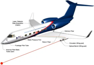
Figure 1.Diagram of the LAMS. Light generated by the laser in the cabin is transmitted by optical fibres to a wing pod, where it is transmitted in a beam that has a focal point well ahead of the aircraft (farther ahead than suggested by this not-to-scale diagram). The light backscattered from aerosol particles in the focal region is collected by the lens, and a circulator mixes a portion of the trans-mitted signal with the returned signal. The resulting signal, with interference patterns that measure the Doppler shift of the backscat-tered light, is returned via optical fibre to the cabin for digitization. Also illustrated in this figure are the approximate locations of the static pressure ports and the fuselage pitot tube used by the research data system to measure static and dynamic pressures. This figure appears in Applied Optics in the article by Spuler et al. (2011) and is used here with permission from the Optical Society of America.
was 30 m ahead of the instrument, or 16 m ahead of the nose of the aircraft. For the C-130, the focal distance was 15 m ahead of the instrument. Different lensfnumbers were used, such that in both cases the returned signal was dominantly from a volume extending about 2.5 m along the direction of flight, as given by the full-width half-maximum distance of the telescope gain pattern. A small inertial system (Sys-tron Donner C-MIGITS INS/GPS) mounted in the wing pod with the LAMS measured deviations in orientation caused by wing flex or other vibrations of the pod relative to the aircraft centre axis, where the aircraft orientation was mea-sured by a separate Honeywell Laseref IV or V SM inertial reference system. Both provided measurements of attitude angles and aircraft velocity with respective standard uncer-tainties of about 1 mrad and about 0.1 m s−1, after incorpora-tion of measurements from global posiincorpora-tioning system (GPS) receivers.
Earlier versions of laser wind sensors operating at 10.6 µm wavelength were designed for use on NCAR aircraft in the 1980s and 1990s, as discussed by Keeler et al. (1987), Kristensen and Lenschow (1987) and Mayor et al. (1997), but developments in fibre optics now have made a much im-proved system practical. For the present system, the wave-length used is about 1.56 µm; Spuler et al. (2011) estimated that a particle concentration of about 2 cm−3with a diameter
in the range from 0.1 to 3 µm is needed to provide a de-tectable signal, but the sensitivity has been improved since that early test. Successful detection of the backscattered sig-nal has been possible at altitudes extending to above 13 km although with present sensitivity there are still times when the signal is too small for a valid measurement.
The precision estimated in Spuler et al. (2011) is 0.05 m s−1 for 1 s samples (as will be used in the present analyses); however, the system can provide data at much higher rates because individual samples are recorded at 100 Hz after the averaging of individual spectra sampled at rates of about 200 kHz. The light source is a distributed feedback fibre laser module (NKT Basik E15) with wave-length 1559.996 nm in vacuum and 0.1 pm(◦C)−1stability. The laser is maintained within 1◦C of a constant
tempera-ture, so wavelength drift is below 0.001 nm. The conversion from measured Doppler shift to airspeed involves only the wavelength of the laser and the speed of light. The error at-tributed to variation in the laser wavelength is equivalent to 0.01 mm s−1for wind measurements that are typically about 200 m s−1. In comparison to the overall 50 mm s−1precision of the measurement, this error makes a negligible contribu-tion to precision or uncertainty.
The peak Doppler frequency can be measured with a stan-dard uncertainty that, converted to airspeed, is less than 0.1 m s−1. The precision estimate from Spuler et al. (2011) also supports an estimated uncertainty in this range if there is no bias in the selection of the peak in the shifted fre-quency spectrum, as is supported by careful examination of the recorded spectra and the operation of the algorithm that identifies the peak (discussed at the end of Sect. 3 of that ref-erence). When the signal-to-noise ratio indicates that there is inadequate signal from which to obtain a Doppler shift, the measurements are flagged as missing and are not used in the analysis to follow.
3 Calibrating the pressure-sensing system 3.1 Dynamic pressure
The most straightforward application of measurements from the LAMS is to predict the dynamic pressureq. Ifp is the ambient pressure,cvandcp the respective specific heats of air at constant volume or constant pressure,T the absolute temperature, andRathe gas constant for air, the Mach num-berM(ratio of flight speedvto the speed of sound√γ RaT, withγ=cp/cv) is given by the following equation (cf. e.g.
Lenschow, 1972):
M=√ v
γ RaT = (
2cv Ra
"p +q p
Ra/cp −1
#)1/2
Solving for the dynamic pressure gives
q=p (
v2
2cpT +
1 cp/Ra
−1 )
, (2)
which shows that, with knowledge ofpandT, LAMS (mea-suring v) can provide an independent prediction of the dy-namic pressureq. Furthermore, small errors inpandT will have a small effect on the deduced dynamic pressure because expected errors are a small fraction of the total ambient pres-sure or the absolute temperature. For typical flight condi-tions, an uncertainty in temperature of 1 K leads to a frac-tional uncertainty in q of about 0.5 % or, for q=60 hPa, about 0.3 hPa. Because the calibration of the temperature sensors is tested in Sect. 5 of this paper to a standard uncer-tainty of 0.3◦C, this uncertainty in temperature leads to an uncertainty in calibrated dynamic pressure of about 0.1 hPa.
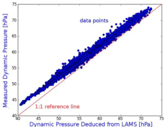
Corrections are usually applied to measurements of dynamic pressure on research aircraft, including the NSF/NCAR research aircraft, so comparingqas provided by Eq. (2) to the uncorrected measurement of dynamic pressure
qmis an exaggeration of the improvement that LAMS pro-vides. Nevertheless, Fig. 2 shows that the difference between the predicted value from LAMS using Eq. (2) and the direct measurement (from one of the pitot tubes on the C-130 refer-enced to the static pressure source) is substantial and exhibits both a large bias and significant scatter. Applying corrections to the direct measurement is therefore important if the air mo-tion relative to the aircraft is to be determined accurately. 3.2 Ambient or static pressure
The normal measurement of total pressurept=p+qis ob-tained on the GV and C-130 and many other research air-craft by measuring the pressure delivered by a pitot tube aligned approximately along the airflow. This measurement is made by adding two measurements, one of ambient pres-sure p (measured by a Parascientific Model 1000 absolute pressure transducer with 0.1 hPa measurement uncertainty, connected in parallel to static ports on each side of the fuse-lage of the aircraft) and a second of dynamic pressure q
(measured by a Honeywell PPT (0–5 PSI) differential sensor with 0.02 hPa measurement uncertainty, connected between the static ports and the pitot tube). These measurements are sampled at 50 Hz, filtered to 25 Hz and optionally averaged to 1 Hz. Two independent systems with separate static ports are available on the C-130, but only one on the GV. On both aircraft, there are also measurements from another indepen-dent system that supplies information to the flight crew and is also recorded for research use.
Pitot tubes are generally insensitive to small deviations from normal flow angles, typically delivering accurate total pressure within about 0.1 % for flow angles up to several de-grees from the centreline of the pitot tube (e.g. Gracey et al., 1951; Balachandran, 2006; Tropez et al., 2007). However,
Figure 2. The direct measurement of dynamic pressure (qm) on the C-130 vs. that deduced using the LAMS measurement of air-speed, via Eqs. (3) and (5). All 1 s average points from one C-130 research flight on which the LAMS was tested (17 November 2011) are shown.
static ports can deliver pressures that depart much more from the true ambient pressure at the flight level when flow around the fuselage varies, and they can also produce biases even at normal flight angles, so the largest error is expected inp
and consequently inqwhile their sumpthas a substantially smaller error. This was checked on the GV and on the C-130 by comparing the redundant sources for these measure-ments. The results forptwere remarkably consistent among all pairs (agreeing to within 0.1 hPa) but there was significant variability in the redundant measurements of bothp andq, often at the level of a few hPa.
For example, Fig. 3 compares two redundant measure-ments of total pressure on the C-130, each based on a dif-ferent pitot source and static source. This and other similar comparisons suggest that a good approximation is to con-siderptaccurately measured and to assume that1q, the er-ror in the measurementqmof dynamic pressure, is equal to the negative of1p, the error in the measurementpmof am-bient pressure, because both arise from the “static defect” or error in the pressure present at the static source:
1q=qm−q= −1p= −(pm−p) . (3)
As a result, the correction to dynamic pressure obtained from LAMS also provides a correction to ambient pres-sure, and these corrections can be applied simultaneously in Eq. (3) using Eq. (2):
1q=qm−pχ (v, T ),
where, to simplify the notation,χ (v, T )is
χ (v, T )= v2
2cpT +
1 cp/Ra
−1. (4)
Then, becausep=pm−1p,
pc= −1p=
qm−pmχ
Figure 3. Measurements made at 1 Hz during the 17 Novem-ber 2011 flight of the C-130. All measurements are included for times when the true airspeed exceeded 50 m s−1(to exclude a short period with flaps deployed at the end of the flight). The measure-ments plotted are the total pressurept, measured by two indepen-dent systems using two different pitot tubes and sets of static but-tons. The root-mean-square deviation from this line is 0.1 hPa, and the similar deviation from a best-fit line is less than 0.04 hPa.
which gives the correction to ambient pressurepcin terms of the measurements of ambient and dynamic pressure, the air-speed measured by the LAMS and the absolute temperature. The negative sign arises because the correction needed is the negative of the measurement error.
The temperature is needed to calculate χ, but it can be assumed tentatively that the uncertainty in the temperature measurement is adequate for this analysis. Once pressure corrections are found, this assumption can be checked and the process can be iterated as necessary. Equations (4) and (5) then can be used with measurements from the LAMS to estimate both the correction to be applied to the ambient pres-sure and, with reversed sign, the correction to be applied to the dynamic pressure.
The results obtained in this way are dependent on the specific locations of the pressure ports providing the static source. Haering Jr. (1995) discusses general considerations regarding placement and characteristics of these ports. On the research aircraft discussed in the present paper, to avoid interference with the standard ports used by the avionics sys-tems, separate ports have been installed to provide this static source. The locations on the GV, shown in Fig. 1, are at fuse-lage station 247.0 and water line 80.2 (by convention quoted in inches, equal to 6.274 and 2.032 m respectively), sym-metrically on the starboard and port sides. The primary pitot tube on the GV is located at fuselage station 54.0 (1.572 m) and butt line −19.0 (−0.483 m, negative indicating on the port side). The correction procedure developed in Sect. 3.5 depends on measurements of flow angle as determined by pressure measurements from the radome gust system (with
pressure ports on the nose of the aircraft), so the pitot tube needs to be relatively close to the nose in order for those mea-surements to provide accurate characterization of flow con-ditions in turbulent concon-ditions. Other locations for the static sources will have different errors and different dependence on flow characteristics. This approach to calibration, how-ever, should work with any pitot source that is insensitive to flow angles and is installed outside the boundary layer of the fuselage.
3.3 Some refinements
The goal of these analyses is to measure state variables with significantly lower uncertainty than has been possible in the past, so this objective requires attention to some minor error sources. Specifically, it was necessary to consider: (i) the hu-midity of the air and its effect on thermodynamic properties like the gas constant and specific heats; (ii) the effect of small departures of the pointing angle of the LAMS beam from the direction of the relative wind and (iii) possible effects of flow angles on the total pressure measured by the pitot tube. 3.3.1 Correction for humidity
The first was determined in a straightforward way by con-sidering the properties determined from weighted averages of the properties of dry air and humid air, in standard ways, as described by Khelif et al. (1999). Many of the preceding equations are affected by these adjustments to the gas con-stant and specific heat for moist air.
3.3.2 Correction for LAMS orientation
3.3.3 Effect of flow not parallel to the pitot tube According to information provided by manufacturers, the typical sensitivity of a pitot tube to flow direction is less than 1 % at flow angles up to 10◦ and less than 0.2 % for flow angles up to 5◦. See also the general discussion in Haering Jr. (1995). The error is in the direction of measuring too low a total pressure as the flow angle increases, and to some ex-tent it is compensated by orienting the pitot tubes along the average flow direction expected in normal flight.
To check this, a flight segment with LAMS operational in-cluded yaw manoeuvres in which the aircraft was flown in conditions of small side-slip (<3◦) in cross-controlled con-ditions so that the aircraft continued in approximately the same direction and at approximately the same airspeed. Un-der those conditions, one would expect that the total pressure measured by the pitot tube would not show a dependence on side-slip angle.
Because a low-tolerance test is desired, small corrections are needed for the observed departures from steady flight speed and in altitude. Over the course of the manoeuvre, GPS measurements of altitude were used with the hydrostatic equation to estimate and correct for changes in the ambient pressure usingδp= −(p/RaT )gδz, whereδzis the change in altitude from the start of the flight segment,pis the am-bient pressure, Ra the gas constant for air,T the absolute temperature andgthe acceleration of gravity. In addition, a correction was made for the expected change in total pres-sure arising from small changes in airspeed, as meapres-sured by the LAMS. This is an independent measurement of airspeed that does not rely on the aircraft measurements of ambient and dynamic pressure, so the correction is not affected by possible errors in the measurement of dynamic pressure. The correction applied is given by the following equation:
δq=
p RaT
v2
2cpT +
1
cp Ra−1
v
δv, (6)
which is obtained by differentiating Eq. (2). In this equation,
vis the airspeed measured by LAMS (corrected for flow an-gles as specified above) and the increment is referenced to the arbitrary starting value in the time series so that corrections are made for the non-steady flight speed during the manoeu-vres.
With these corrections, the average total pressure measure-ments as a function of the magnitude of the side-slip angle are as shown in Fig. 4. Within a limit of about 0.1 hPa, there is no dependence on side-slip angle out to about 3◦, a range in side-slip angles and also in attack angles from the mean that is characteristic of normal flight of both NCAR aircraft. This supports neglecting a possible dependence of the total pres-sure meapres-surement on flow angles, at least for the small angles characteristic of normal flight; however, the test is not as rig-orous as might be desired because airflow distortion around
Figure 4.The total pressure (from the sum of the ambient pressure measurement and the dynamic pressure measurement) on the C-130 as a function of the magnitude of the side-slip angle during yaw manoeuvres in which side-slip angles were forced by rudder action while the aircraft continued on approximately a straight-and-level course. The mean total pressure of 760.6 hPa has been subtracted from the measurements. Error bars are standard deviations in the measurements for the total pressure axis and are the range of the bin used in side-slip. Corrections for deviations from a level course and for small variations in airspeed have been applied, as discussed in the text.
the fuselage may cause the flow angle at the pitot tube to dif-fer from the measured side-slip angle.
3.4 Uncertainty in the corrections
When the LAMS is operating, the corrections to ambient and dynamic pressure can be determined directly from Eqs. (3) and (5), and these corrections have much stronger justifi-cation than the empirical corrections used previously. The LAMS evaluation (Spuler et al., 2011) suggests that the un-certainty in line-of-sightvis about 0.05 m s−1, so this is also approximately the uncertainty in the component of the rel-ative wind along the axis of LAMS. The total derivrel-ative of Eq. (2) provides a basis for evaluating the uncertainty in the value ofqestimated from Eq. (2):
δq
p =
v2
2cpT +
1
cp Ra−1 v2
RaT δv
v −
1 2
1T T
. (7)
The temperature uncertainty thus contributes significantly to the uncertainty in q, often more than the uncertainty in v
T =Tr−αT
v2
2cp
, (8)
withTrthe measured or “recovery” temperature,αT the re-covery factor for the sensor measuring Tr, andv provided by LAMS rather than the conventional solution for the Mach number determined from ambient and dynamic pressure. The recovery factor used for the GV in this study (specified later, in Sect. 5.2) was determined by fitting to data in Stickney et al. (1994), where reported measurements span a range in
aT that corresponds to a standard uncertainty of about 0.007
inαT. For a representative airspeed of 220 m s−1this
cor-responds to an uncertainty in temperature of about 0.2◦C. Calibration of the temperature measurement, which includes dependence on the recovery factor, is presented in Sect. 5.2, where it is argued that the temperature is constrained by that calibration within about 0.3◦C of that measured, so usingv
as measured by LAMS keeps the standard uncertainty intro-duced byT within this limit.
Interpreted as an uncertainty in dynamic pressure q, the uncertainty in the prediction of q from LAMS deter-mined from Eq. (7) is typically about 0.13 hPa (for flight at 125 m s−1, where the pressure is 760 hPa and the temperature 0◦C). The uncertainty in the uncorrected measurement of
pm, from instrument characteristics, is also about 0.1 hPa, so using the LAMS correction yields an ambient pressure that has an uncertainty of around 0.16 hPa. Evaluation at 150 hPa leads to a similar estimate of uncertainty. When LAMS is present, it is thus possible to be confident that the measure-ments of the longitudinal component of the relative wind and of the ambient pressure have associated standard uncertain-ties of<0.1 m s−1and 0.16 hPa, respectively.
3.5 Fits to the corrections
There is still value in determining fits to the corrections pro-vided by LAMS in terms of flight characteristics like flight level, angle of attack, Mach number etc. because then correc-tions can be applied in cases where the LAMS is not present or does not detect enough signal to provide a valid airspeed. Such fits can be applied retrospectively to data collected be-fore the LAMS was available, and the fits can also be com-pared to other means of estimating the corrections. A further reason for developing fits is that the LAMS measurement, being offset from the nose of the aircraft, represents a re-gion where there may be a fluctuating difference in airspeed vs. that present at the nose, and averaging over such fluctua-tions as provided by functional fits smooths the predicted cor-rections. Fits to the measurements may therefore be prefer-able to those corrected directly using the LAMS airspeed
v, especially in turbulent regions. For these reasons, fits to the measurements provided by Eq. (5) were explored un-til adequate representations of the predicted fits were found. Variables considered in the fits included ambient pressure,
dynamic pressure, Mach number, angle of attack, side-slip, airspeed and other characteristics of flight. The following analyses use flights during which the LAMS provided valid measurements almost continuously and during which there were many altitude changes and speed variations.
3.5.1 GV
For the GV, the best representation of1p, obtained after try-ing many options, was
1p
p =a0+a1M
2
+a2M3+a3
1pα 1qr
+a4 1p
α 1qr
2 +a5
1p α 1qr
3
, (9)
where 1pα is the pressure difference between
verti-cally separated pressure ports on the radome (normally used to calculate the angle of attack; cf. Brown et al., 1983) and 1qr is the pressure difference measured be-tween the centre port on the radome and the static source. The terms involving 1pα/1qr introduce depen-dence on angle of attack. The dimensionless coefficients {a0, a1, a2, a3, a4, a5} for the best fit to the measurements from a GV flight with LAMS operating were, respectively, {−0.0133,0.0425,−0.0716,−0.360,−3.60,−9.66}, where the quoted significant digits reflect the standard error in de-termining these coefficients. In the analysis of significance of the fit, all these coefficients were needed to represent the variance, at significance levels less than 0.001.
The correlation coefficient between the measured pressure corrections and those predicted by Eq. (9) was 0.98 and the standard error was 0.00089 (i.e. 0.089 % of the measured pressure, or about 0.3 hPa at a typical ambient pressure of
p=350 hPa). This standard error reflects individual mea-surements for which some scatter arises because the LAMS and pressure-sensing systems detect air parcels slightly dis-placed from each other that potentially have different air mo-tions (cf. the discussion of this point in Sect. 4). The high cor-relation coefficient indicates that the fit accounts for>96 % of the variance between the predicted and measured pres-sure corrections. Including additional functional dependence terms in Eq. (9) did not reduce the residual variance beyond this limit, so there is no evident source of this residual vari-ability beyond the fraction that may arise from the samples being at different locations for the two systems.
in the pressure correction. Thus, using the LAMS measure-ment of airspeed has removed a 3.5 hPa error and provided a reference for a parametric fit that has residual uncertainty of<0.3 hPa. Any random error in the uncorrected measure-ment of pressure would appear in this residual uncertainty, as would a random error in the LAMS measurement, and a bias in the measurement of pressure would be corrected by the calibration procedure. Bias in the LAMS measurement of airspeed of, e.g. 0.05 m s−1would still lead to a bias in the calibrated pressure of typically about 0.15 hPa, as argued in Sect. 3.4, but this is still small in comparison to the residual uncertainty arising from the parametrized fit.
A concern regarding Eq. (9) is that during the flight from which this fit was determined the variable1pα/1qrvaried only from about −0.2 to−0.03, while the full flight enve-lope of the GV spans a larger range. There is a danger that the cubic dependence on this term in Eq. (9) might extrap-olate to erroneous corrections outside that range. To guard against such errors, other fits were developed that, although slightly less accurate, should extrapolate to new conditions better. One example is the following:
1p
p =a
′
0+a′1
qm
pm+
a′2M3+a3′1pα 1qr
, (10)
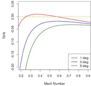
with values of the coefficients {ai,i′ =0−3} respectively {−0.00076, 0.073,−0.0864, 0.0465}. The resulting correc-tion is plotted in Fig. 5, for flight at 500 hPa. This fit to the LAMS measurements accounted for 95 % of the variance, vs. 96 % for Eq. (9), so it may be preferable to use Eq. (10) in cases where flight conditions might fall outside the normal range of angle of attack used to determine Eq. (9).
3.5.2 C-130
Fits to the values of Eq. (5) obtained as above were also ex-plored for a C-130 flight with LAMS operating. For one pair of measurements of ambient pressure and dynamic pressure, the best fit with all highly significant coefficients (signifi-cance level<0.001) was the following:
1p
p =b0+b1 1pα
1qr +
b2M+b3
1pβ 1qr
, (11)
where1pβ is analogous to1pα but for the side-slip angle. The standard error for this fit was 0.0004, corresponding to a pressure uncertainty at 700 hPa of about 0.3 hPa for the individual measurements. The second term gave the largest reduction in residual error; using this variation alone gave a residual standard error of 0.00050. A fit using only the first three terms on the right side of Eq. (11) increased the residual standard error by less than 0.00001, making an ad-ditional error contribution to the corrected pressure of typi-cally 0.014 hPa, which is insignificant in comparison to other expected error sources, so this simpler fit may be prefer-able. The coefficients, with quoted significant digits deter-mined with consideration the standard errors in the fit, are
Figure 5.The correction to pressure (δp) normalized by the magni-tude of the dynamic pressure (q), as a function of Mach number, for three values of the angle of attack. The values plotted are those for the GV as given by Eq. (9) for flight at 500 hPa. The format of the plot is chosen to match conventional presentations in aeronautical publications such as Gracey (1980).
{b′0, b′1, b′2} = {0.00152,0.0205,0.0149}. While the residu-als from this fit are small, the mean offset it produces is about 2 hPa, so (as illustrated by Fig. 2) the effect on the measure-ments of ambient and dynamic pressure is quite significant.
For both aircraft, direct use of the LAMS measurements can reduce the uncertainty in measurements of ambient and dynamic pressure to around 0.15 hPa. Even when the LAMS is not present, parametric fits to LAMS measurements can reduce the uncertainty in pressure to less than 0.3 hPa. 3.6 Comparisons to other evidence
There are several comparisons possible that can test these results. Three are discussed in this section.
3.6.1 Wind measurements in reverse-heading manoeuvres
A reverse-heading manoeuvre is one in which a straight-and-level flight leg is flown for a short time (2 to 5 min) and then the aircraft reverses course and flies the same leg in the oppo-site direction. Usually these are flown approximately along and against the wind direction. A test of the accuracy of the measurement of dynamic pressure is that the longitudi-nal component of the wind should reverse direction but have the same magnitude in reverse-heading manoeuvres when the aircraft is flown over the same (drifting) flight leg twice with opposite headings. To isolate the effect of the measure-ment of q and hence true airspeed, the best wind compo-nent to use is that along the axis of the aircraft, which is
GPS system provides the ground-speed magnitudevgand the ground track angle8, soδ=8−9, where9is the heading of the aircraft. Then, the wind component along the longitu-dinal axis of the aircraft is
vx=vgcos(8−9)−vt, (12)
wherevtis provided either directly from LAMS or from the corrected dynamic pressure via Eq. (9) for the GV or Eq. (11) for the C-130. The expectation is that the longitudinal com-ponent of the wind given by Eq. (12) will reverse sign be-tween the two legs of the reverse-heading manoeuvre. Within statistics imposed by atmospheric fluctuations, this is then a test of the validity of the longitudinal component of the wind measurements.
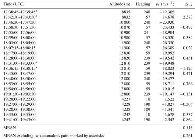
A GV flight with a large number of reverse-heading ma-noeuvres, but without the LAMS, was used for the test de-scribed in this section. Table 1 shows the results for 12 reverse-heading pairs of legs from this flight. The mean difference on legs along opposing headings was −0.12± 0.91 m s−1, but there are two pairs of legs (marked with as-terisks in the table) that appear to be outliers such as would be expected if the wind conditions changed between the two legs. If these are excluded, the remainder give a standard deviation such that the excluded legs would be more than two standard deviations from the mean. Excluding these two legs, there are 10 legs with a mean difference of −0.26± 0.43 m s−1, with standard error in the mean of 0.14 m s−1. This result suggests that the error in measurement of longi-tudinal wind is−0.13±0.07 m s−1, which is consistent with estimates of the uncertainty associated with the applied cor-rection to airspeed based on Eq. (10). This provides support-ing evidence that the standard uncertainty in the measure-ment of the longitudinal component of the relative wind after correction is about 0.1 m s−1.
3.6.2 The avionics pressure system of the GV
The ambient pressure measurement from the avionics system on the GV is more reliable than those on many research air-craft because the GV is certified to fly on RVSM (reduced vertical separation minimum) levels; therefore, the flight-deck pressure measurement has met strict Federal Aviation Administration requirements. Appendix G to Federal Avia-tion RegulaAvia-tions Part 91 specifies that the maximum allow-able error in altitude is 80 ft, or about 24 m. In the RVSM altitude range (flight levels 290 to 410), this corresponds to a requirement that the error in pressure be in the range of about 0.68 hPa (near FL410) to 1.1 hPa (near FL290). For the GV flight used above, the mean difference between the pressure provided by the avionics system and that measured with correction by LAMS, for the RVSM altitude range, was +0.36 hPa with standard deviation 0.19 hPa, so within the tolerance required by RVSM standards, the avionics pressure is consistent with the measured pressure as calibrated in this study.
Figure 6. The d value measurements as a function of time for a flight segment at about 450 hPa, and the corresponding values of the Mach number (plotted relative to the right axis). It might be ex-pected that thedvalue would change smoothly, as suggested by the solid red line. GV flight of 12 August 2010, Colorado, USA to St. Croix, Virgin Islands. Gaps in data show portions omitted because the LAMS signal was too weak to be reliable.
3.6.3 “dvalue” measurements during speed runs
The dominant dependence in the pressure correction repre-sented in Eq. (9) is on Mach number, so testing this de-pendence is a useful constraint on the validity of the cor-rections. Repeatedly during the flight used to determine the pressure calibration in this study, the GV was flown in level flight, moving from near its low-speed limit to near its high-speed limit. If the pressure corrections are adequate, such manoeuvres should not introduce perturbations into the mea-sured pressure. A stringent test of this expected indepen-dence of Mach number is to consider the difference between the geometric altitude and the pressure altitude, or “dvalue” (cf. Bellamy, 1945) during the manoeuvre. This compensates for small altitude changes of the aircraft and should show a continuous change not perturbed by the airspeed changes or small altitude changes.
Table 1.Pairs of reverse-heading manoeuvres. Average values for altitude, heading and the longitudinal component of the wind (vx) are listed. Data from the GV flight of 6 August 2010.
Time (UTC) Altitude (m) Heading vx(m s−1) 1vx
17:38:45–17:39:45∗ 8835 240 −12.305
17:42:30–17:43:30∗ 8832 57 14.678 2.373
17:46:30–17:47:30 10 060 240 −23.930
17:50:30–17:51:30 10 070 57 23.433 −0.497
17:55:00–17:56:00 10 980 241 −18.904
17:59:00–18:00:00 10 980 57 18.520 −0.384
18:03:00–18:04:00 11 900 240 −26.330
18:07:15–18:08:15 11 900 57 26.309 0.022
18:17:00–18:19:00 12 830 59 19.993
18:28:00–18:30:00 12 820 239 −19.542 0.451
18:31:00–18:33:00∗ 12 810 239 −19.948
18:36:15–18:38:15∗ 12 810 59 18.823 −1.125
18:45:00–18:47:00 12 810 239 −19.294 −0.471
18:48:00–18:50:00 12 800 240 −19.477
18:53:00–18:55:00 12 800 59 18.711 −0.766
18:54:00–18:56:00 12 800 59 19.015
19:01:30–19:03:30 12 800 239 −19.147 −0.131
19:20:00–19:22:00 4227 10 1.522
19:27:00–19:29:00 4228 190 −1.827 −0.305
19:28:00–19:30:00 4228 189 −1.341
19:33:00–19:35:00 4242 10 1.678 0.337
19:41:00–19:43:00 4242 190 −2.542 −0.864
MEAN −0.113
MEAN excluding two anomalous pairs marked by asterisks −0.261
consistency of the trend suggests that the dependence of the correction on Mach number is appropriate to within an un-certainty of about 0.2 hPa.
4 Correcting the measured airspeed
The LAMS provides a direct measurement of line-of-sight airspeed and, with the correction as in Sect. 3.3.2, true air-speed, but it is still useful to use the pressures as determined in the preceding section to determine airspeed by solving Eq. (2) for v as a function of p and q. Because the vol-ume in which LAMS senses the airspeed is displaced from the nose of the aircraft, the airspeed that it senses may dif-fer slightly from that sensed at the radome of the aircraft. For the GV, the difference between the airspeed measured by LAMS and that determined from the corrected dynamic and ambient pressures has a standard deviation of 0.35 m s−1. Es-timates based on measured turbulence levels indicate that this is similar to the difference expected for sample locations sep-arated by about 16 m, the distance between the LAMS sens-ing volume and the nose of the GV, but for this comparison the samples are 1 s averages that would be expected to dif-fer by much less than this, perhaps reduced by a factor of around√200/16. This suggests that differences in location
account for perhaps 30 % of the observed standard deviation. This fraction is still significant, so even when the LAMS is present, airspeed used to determine the wind may be better if based on the corrected pressures that use the parametric fits rather than that measured directly by the LAMS.
On the GV, the mean change in true airspeed introduced by this calibration is−0.8 m s−1. The standard error in the determination of this offset is much smaller than the ex-pected uncertainty in the measurement from LAMS (which is <0.1 m s−1), so calibration using LAMS has removed a−0.8 m s−1error and reduced the uncertainty in this mea-surement to <0.1 m s−1. For the C-130, the correspond-ing correction is+0.5 m s−1. These measurements are used along with measurements from GPS and an inertial refer-ence system (IRS) to determine the wind, and the GPS/IRS also provides measurements with an uncertainty of about 0.1 m s−1, so the calibration based on LAMS has reduced the uncertainty in the component of the wind along the aircraft axis to<0.2 m s−1.
5 Checking the calibrations of thermometers
sensors on the research aircraft by calculating height dif-ferences from integration of the hydrostatic equation and comparing them to measured height differences. The lat-ter are provided with low uncertainty by modern GPS mea-surements of geometric altitude. The improved measurement of pressure provided by LAMS reduces the uncertainty in the measurement of pressure differences and enables a more stringent test of the validity of the measurements of temper-ature.
The hydrostatic equation can be expressed in this form:
δpi = − g pi
RaTi
δzi, (13)
where {pi, Ti}are the values of ambient pressure and ab-solute temperature for the ith measurement and δpi is the change in pressure for theith step, during which the geomet-ric altitude changes byδzi. This equation can be rearranged
to obtain an estimate of the temperature:
Ti= −g Ra
δzi δlnpi
. (14)
Measurement uncertainty of 0.1 % in derived temperature (i.e. a typical uncertainty of 0.3◦C) requires at least 0.1 % precision in the measurement ofδz, a precision now provided by differential GPS receivers (such as the NovAtel Model OEM-4 L1/L2 Differential GPS system in use on both NCAR aircraft) for height differences as small as 100 m. The re-quirement is more stringent for the measurement of pressure. At 10 m s−1rate of climb, the pressure change over 10 s is less than 10 hPa, and it seems likely that differences in pres-sure cannot be meapres-sured confidently to better than 0.1 hPa, so this would introduce an error of 1 % in the deduced (ab-solute) temperature. This is inadequate, so a larger altitude difference or the average of many measurements is required to obtain a useful estimate of the temperature.
5.1 C-130
About 30 min of flight with the LAMS on the C-130 was devoted to repeated climbs and descents and included about 1800 measurements of 1 s differences, so it might be ex-pected that the standard error in the determination of tem-perature from Eq. (14) could be reduced by√1800=42, or to around 0.5◦C, by this procedure. Alternately, an
appropri-ately weighted “mean” temperature between two levels can be determined from Eq. (14). For this flight segment, climbs were repeated from about 12 000 to 16 000 ft (about 3.7 to 4.9 km), or over a pressure range of about 100 hPa, and the course reversed midway through the flight segment, so this should help compensate for any true horizontal gradient in pressure. An uncertainty of 0.1 hPa in a 100 hPa pressure change leads to about an uncertainty of 0.1 % or, in absolute temperature, an uncertainty of about 0.3◦C in the mean tem-perature between the layers. It should therefore be possible
to test the temperature measurements with about this level of confidence.
Specifically, three sums were calculated between different flight levels:
S1= X
i Ra,i
gi
ln p
i pi−1
, (15)
S2= X
i
(zi−zi−1), (16)
S3= X
i
zi−zi−1
Tm,i
, (17)
whereRa,i andgi are respectively the gas constant (adjusted
for humidity) and the acceleration of gravity (adjusted for latitude and altitude) andTm,iis the measured temperature in
absolute units, corrected for airspeed but based on the stan-dard sensors being tested. The predicted mean temperature for the layer, weighted by altitude, is given byTp= −S2/S1, while the corresponding weighted-mean measured tempera-ture isTm=S2/S3, so a comparison ofTm toTptests the validity of the temperature measurement.
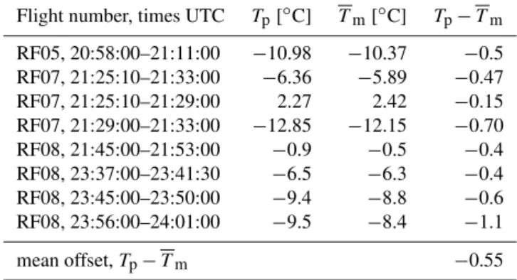
Table 2 shows some measurements from selected flight legs of the C-130. The evidence from these climbs indicates that the measured temperature was about 0.5◦C too high and that the offset perhaps increases as the temperature decreases. After this result was obtained, an investigation discovered an error of about this magnitude in the calibration of the temper-ature sensor, which arose from a flawed bath calibration. This illustrates the value of the independent calibration provided by the LAMS.
5.2 GV
A similar approach could be taken for the GV, with the promise of a larger range of calibration points because of the large altitude changes occurring during many of the flights. However, because there have been many flights with frequent altitude changes, it was decided instead to use a large data set with many climbs and descents to determine a polynomial correction to the temperature via minimization of the error between actual altitude changes and those predicted from in-tegration of the hydrostatic equation. The chi-square (χ2) to be minimized was
χ2=X
i
1
σ2
z
(hi−Zi)2, (18)
whereZi is the geometric altitude measured by GPS,σz is
the uncertainty in the height measurement and the predicted heighthiwas determined by the integration of the hydrostatic
equation in the form
hi=hi−1−
Ra(f (Ti))
g ln
pi pi−1
, (19)
f (Ti)=
(c0+(1+c1)Ti+T0) 1+αT 2RCavM2
Table 2.Comparisons of predicted and measured temperatures from climbs and descents of the C-130. The segments are from flights RF05, RF06 and RF08 flown respectively on 7, 15 and 17 Novem-ber 2011.Tpis the predicted temperature andTmis the weighted mean of the measured values of temperature, as defined in the text.
Flight number, times UTC Tp[◦C] Tm[◦C] Tp−Tm
RF05, 20:58:00–21:11:00 −10.98 −10.37 −0.5 RF07, 21:25:10–21:33:00 −6.36 −5.89 −0.47 RF07, 21:25:10–21:29:00 2.27 2.42 −0.15 RF07, 21:29:00–21:33:00 −12.85 −12.15 −0.70 RF08, 21:45:00–21:53:00 −0.9 −0.5 −0.4 RF08, 23:37:00–23:41:30 −6.5 −6.3 −0.4 RF08, 23:45:00–23:50:00 −9.4 −8.8 −0.6 RF08, 23:56:00–24:01:00 −9.5 −8.4 −1.1
mean offset,Tp−Tm −0.55
wherec0andc1are coefficients to be found by minimization of Eq. (18). In these equations,Ra is the moist-air gas con-stant,gthe acceleration of gravity (adjusted for latitude and altitude) and{pi}is the time sequence of measured pressures. The functionf (Ti)allows the adjustable coefficientsc0and
c1 to be applied to the measured temperatureTi, with con-version to ambient temperature on the basis of the recovery factor (αT), the Mach number (M) and the specific heat at
constant volume (cv). The resulting temperature is converted
to an absolute temperature by the addition ofT0=273.15 K. Because the climbs and descents were made en route and so spanned some horizontal distance, the vertical integration will match the pressure change only if the atmosphere is hori-zontally homogeneous. If not, the results will be biased as the fit attempts to compensate for horizontal gradients, and this can introduce an error into the minimization results. To con-sider how serious this problem is, it is useful to assess how a pressure gradient will affect the results. Suppose the hori-zontal pressure gradient along the flight path is dp/ds=Gp. Then, there will be a contribution to the pressure change aris-ing just from the pressure gradient over a period1t, of mag-nitudeGpv1t, wherevis the airspeed. Therefore, in Eq. (19)
the pressure ratio in the logarithmic factor must be modified to be(pi−Gpvi1t )/pi−1.
It is convenient to express this in terms of d value, the difference between geometric altitude and pressure altitude, because that is measured routinely. Part of the change in
d value during a climb results from the horizontal pressure gradient, while another part arises from the climb in an at-mosphere that differs from the standard atat-mosphere. The ex-pected change indi, the measurement ofdvalue, is then
di−di−1= − R
af (Ti)
g −
RsTs(p)
gs
ln pi
pi−1
−GpRaTivi1t
gpi
, (21)
whereRs and gs are the gas constant and acceleration of gravity defined by the US standard atmosphere and Ts(p) is the absolute temperature corresponding in the standard at-mosphere to pressurep. The first term on the right side arises from the climb or descent, while the last term is the contri-bution from the horizontal pressure gradient. The horizontal pressure gradientGpcan then be deduced from the
measure-ments ofd value by rearranging Eq. (21):
Gpvi1t= gpi RaTi×
− R
af (Ti)
g −
RsTs(pi) gs
ln pi
pi−1
−(di−di−1)
. (22)
Then, the altitude-change equation, Eq. (19), should be re-placed by
hi=hi−1−
Ra(f (Ti))
g ln
p
i−Gpvi1t pi−1
, (23)
withGpvi1t evaluated using Eq. (22).
The measurements used were from 10 flights that com-prised the fifth circuit of the High-performance Instrumented Airborne Platform for Environmental Research (HIAPER) Pole-to-Pole (HIPPO) experiment (Wofsy et al., 2011), start-ing and endstart-ing in Colorado, USA, but extendstart-ing north of the Arctic Circle and south to beyond New Zealand. The flight patterns featured repeated climbs and descents to measure profiles through the atmosphere, so the 122 profiles measured (many covering more than 8 km in altitude) provided a good set of measurements for this study. Several data-quality re-strictions were applied to avoid periods of problematic data, notably when ice accumulation or frozen water affected the wind-sensing system and so the measurement of attack an-gle (needed for the correction to ambient pressure). Periods with climb or descent rates less than 2 m s−1were excluded as a way of excluding level flight segments that contributed noise to the analysis. Also, rare periods of climbs or descents exceeding 7.5 m s−1 were also excluded because those pe-riods produced large discrepancies in the results compared to normal climbs and descents, perhaps because of problems with sensor response. Flight periods with airspeed less than 130 m s−1were also excluded to avoid times when the flaps might have been deployed, potentially affecting the pressure measurements. With these exclusions, the data set consisted of about 26 000 samples during climbs and descents.
For measurements made at a rate of 1 Hz, the uncertainty
σz in measurement of the height difference arises
primar-ily from the uncertainty in the pressure change, as discussed above. The best-fit value ofχ2 as defined by Eq. (18) was consistent with a value of about 1.6 m forσz, and this would
so this uncertainty in altitude is consistent with other es-timates in this paper. The minimization was done in vari-ous ways, including evaluating results over matrices of val-ues of the fit parametersc0andc1, conjugate-gradient step-ping and use of the “R” routineoptim(R Core Team, 2013) which implements the Nelder and Mead (1965) minimiza-tion algorithm. All produced consistent results, with con-vergence to values of {c0, c1} = {0.32◦C,0.007}. This ad-justment from the measurements would change the mea-sured total temperature over the course of these flights by +0.29±0.13 K, so the fit indicates that the error in the mea-sured temperature is within these limits. This result applies to the measurement of total temperature, but the minimization of Eq. (18) depended on the accuracy of the ambient tem-perature after application of the recovery factor (usingαT =
0.988+0.053 log10M+0.090 log10M2+0.091 log10M3, ob-tained as explained in Sect. 3.4), so the constraint on mea-surement uncertainty tests for errors in the recovery factor as well as the calibration of the temperature sensor and digiti-zation system.
The uncertainty in the determination of the fit parame-ters{c0, c1}is about {0.02,0.001}, but the uncertainty ma-trix is highly correlated such that the range of values giving an increase inχ2equal to the mean contribution from each point spans from {0.030,0.006} to {0.034,0.008}. Within this range, the mean change in temperature implied by the fit remains in the range 0.28 to 0.31 K and the standard devi-ation in the correction remains smaller than 0.15 K, so there is low uncertainty in the implied adjustment needed for tem-perature.
A potentially more significant source of error, however, is the effect of measurements that for some reason are ques-tionable or erroneous. As discussed above, such measure-ments were excluded where they were identified, but some may remain. To check on the effects of variations in the surements entering the minimization, the sequence of mea-surements was split into five segments and fit coefficients were determined for each. The means of these fit coefficients were {0.37,0.018}and when used individually to evaluate the adjustment needed in the full data set, these fits indi-cated an adjustment of 0.30±0.30.These estimates of un-certainty then indicate a required adjustment in temperature of about+0.3±0.3◦C, with the adjusted total absolute tem-perature T′ given in relation to measured total temperature
T by T′=T0+c0+(1+c1) (T−T0), wherec0=0.32◦C andc1=0.007. This estimated correction and associated un-certainty, obtained because the LAMS provides a calibration of the pressure-sensing system and so with GPS enables ac-curate integration of the hydrostatic equation, are obtained independent of reference standards or intercomparisons with other sensors and are the best available estimate of uncer-tainty in the temperature measurement from the GV.
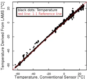
Figure 7.Temperature determined from LAMS using Eq. (24) plot-ted as a function of the corresponding direct measurement of tem-perature for the ferry flight from Colorado, USA to St. Croix, Virgin Islands, on 10 August 2010. Each plotted point represents a mea-surement representing 1 s of flight.
6 Using the LAMS to measure temperature
As discussed above, the LAMS provides a measurement of the true airspeed v and also enables corrections that im-prove the measurements of the ambient and dynamic pres-sure. Those two pressures are sufficient to determine the Mach numberM=v/vs, wherevs=√γ RaT is the speed of sound in air. An equation for temperature can be obtained from Eq. (2) rewritten in the form
T = v
2
2cp
pt p
Ra/cp −1
. (24)
Once calibrated, measurements ofpandptthus can be com-bined withvfrom LAMS to determine the temperature with-out any further reference to temperature sensors on the air-craft.
Figure 7 shows the measurements obtained using Eq. (24) in comparison to the primary conventional measurement of temperature. The mean difference (LAMS temperature mi-nus conventional temperature) is 0.02◦C and the standard deviation is 1.1◦C. The fairly large standard deviation arises mostly from areas of significant turbulence. A histogram of the difference shows that the central peak is characterized by a standard deviation of about 0.5◦C and extremes account for the increase to 1.1◦C in the full sample.
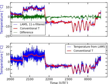
Figure 8. Temperature determined from LAMS plotted with the standard measurement of temperature for a flight segment from the C-130 flight of 17 November 2011, and the difference between the two measurements. The bottom panel shows the 1 Hz measurements from LAMS; in the top panel, these have been smoothed by an 11 s box average.
from the two systems have lower coherence at high rates, and the calculation of temperature is very sensitive to small errors in the pressure measurements.
This new measurement of temperature is valuable as a check on the temperature sensors because miscalibration or changes in the sensors will appear as a discrepancy in com-parison to this measurement. However, temperature measure-ment by LAMS also has a very useful potential application in clouds, where backscatter from the cloud particles makes the LAMS signal very strong and where this measurement should continue to be valid. Measurement of temperature in cloud has been challenging because immersion sensors can become wet and, in the dynamically heated airflow, expe-rience wet-bulb cooling to a variable extent dependent on the wetting (e.g. Heymsfield et al., 1979; Wang and Geerts, 2009). If the measurement of temperature available from LAMS remains valid in cloud, it can provide important infor-mation on the buoyancy of clouds and would support stud-ies of entrainment via mixing-diagram analysis of the type undertaken by Paluch (1979) or Betts (1983), which can be compromised when using conventional temperature sensors. Figure 9 illustrates the capability of the LAMS to mea-sure temperature in cirrus clouds. These meamea-surements were made during a descent through a cirrus layer, where the backscattered signal was dominated by the ice crystals that were present in concentrations varying from about 0.1 L−1 to more than 100 L−1. This demonstrates that the LAMS is able to continue to operate in such conditions and that it con-tinues to provide a useful temperature independent of the im-mersion temperature probes.
Figure 9.Top panel: temperature determined from LAMS measure-ments of airspeed using Eq. (24) compared to the temperature mea-sured by a conventional immersion temperature sensor during a de-scent through a cirrus cloud layer. Bottom panel: the measured ice concentration from a two-dimensional cloud (2-DC) imaging probe.
7 Summary and conclusions
A new laser air-motion sensor, capable of measuring airspeed via the Doppler shift in a laser beam focused about 15 to 30 m ahead of the aircraft, has been used to determine corrections to be applied to the wind component along the axis of the aircraft. With these corrections, the standard uncertainty in this component of the wind has been reduced to less than 0.1 m s−1. Fits to the corrections deduced from this system, as functions of the measurements of ambient and dynamic pressure as well as angle of attack, support this limit on un-certainty even when the LAMS system is not available. Be-cause the basis for the measurement is the Doppler shift in the frequency of backscattered light, the measurement is not dependent on calibration, and because the measurement is made well ahead of the aircraft, it is unaffected by flow dis-tortion around the aircraft.
Once an accurate measurement of airspeed is available, the expected pressure excess above ambient pressure pro-duced by that airflow at the inlet of a pitot tube can be cal-culated. The pressure at flight level can then be determined with low uncertainty by subtracting that excess pressure from the measured total pressure at the pitot tube. The estimated uncertainty in that measurement is less than 0.3 hPa, and the precision (relevant to pressure mapping while the aircraft re-mains in steady flight conditions) is about 0.1 hPa. Calibra-tion to this level of precision enables improved measurement of mesoscale pressure fields in the atmosphere, following the methods developed by Parish et al. (2007) and Parish and Leon (2013) based on GPS technology and by earlier authors including Brown et al. (1981), Shapiro and Kennedy (1981) and LeMone and Tarleton (1986) on the basis of other mea-surements of geometric altitude.
With accurate measurement of pressure, combined with excellent measurements of geometric altitude from modern GPS, it is possible to deduce constraints on the tempera-ture measurement from integrations of the hydrostatic equa-tion during climbs and descents. For the GV, a data set con-sisting of 122 extended climbs and descents, typically over more than 8 km, was used to determine that the measured temperature was within about 0.3◦C of the values required to minimize differences between calculated and true altitude changes. The correction required was a function of temper-ature but typically was +0.3 ±0.3◦C. This correction in-cluded all effects entering the measurement of ambient tem-perature at flight level, including corrections dependent on the recovery factor of the temperature probes, which are a significant source of uncertainty because of the large (of-ten 25◦C) corrections required for dynamic heating at GV flight speeds.
Finally, it was shown that the LAMS, combined with parametrized fits to correction factors for the measured dy-namic and ambient pressure, can provide a measurement of temperature that is independent of any other temperature sen-sor. That measurement continues to be valid in all-ice clouds,
Figure 10.Top panel: temperature determined by the LAMS during a C-130 cloud pass on 15 November 2011. The temperature mea-sured by a conventional temperature probe is also shown. Middle panel: extinction length or distance corresponding to unity optical depth, determined from the measured droplet size distribution. Bot-tom panel: cloud droplet concentration measured by a cloud droplet probe.
but the limited measurements available in water clouds ap-pear less satisfactory. The latter problem is not understood, but is worth further investigation because most immersion sensors are affected by cloud water and produce erroneously low values in water clouds.
A three-dimensional version of the LAMS is now under development and will be ready for flight testing soon. That will extend the improvements available from LAMS to all three components of the measured wind.
Acknowledgements. The instrument development and data collec-tion were supported by the NCAR Earth Observing Laboratory. Data used in this study were collected during field campaigns led by S. Wofsy (HIPPO), C. Davis (PREDICT) and J. Stith (IDEAS), during which the Research Aviation Facility pilots, mechanics, technicians, and software engineers operated the Gulfstream GV and Lockheed C-130 research aircraft. The authors also thank Jorgen Jensen and Jeff Stith for comments and advice on the manuscript. D. Khelif and two anonymous reviewers provided exceptionally helpful reviews that identified errors and led to significant improvement in the manuscript. The National Center for Atmospheric Research is sponsored by the National Science Foundation.
References
Balachandran, P.: Fundamentals of Compressible Fluid Dy-namics, Prentice-Hall of India Pvt-Ltd, available at: http: //books.google.com/books?id=KEzdXmXgaHkC (last access: 21 September 2014), 2006.
Bellamy, J. C.: The use of pressure altitude and altimeter correc-tions in meteorology, J. Meteorol., 2, 1–79, doi:10.1175/1520-0469(1945)002<0001:TUOPAA>2.0.CO;2, 1945.
Betts, A. K.: Thermodynamics of mixed stratocumulus layers – saturation point budgets, J. Atmos. Sci., 40, 2655–2670, doi:10.1175/1520-0469(1983)040<2655:TOMSLS>2.0.CO;2, 1983.
Brown, E. N.: Position Error Calibration of a Pressure Sur-vey Aircraft Using a Trailing Cone, NCAR technical note NCAR/TN-313+STR, Atmospheric Technology Division, NCAR, Boulder, CO, USA, available at: http://nldr.library.ucar. edu/repository/collections/TECH-NOTE-000-000-000-579 (last access: 21 September 2014), 1988.
Brown, E. N., Shapiro, M. A., Kennedy, P. J., and Friehe, C. A.: The application of airborne radar altimetry to the mea-surement of height and slope of isobaric surfaces, J. Appl. Meteorol., 20, 1070–1075, doi:10.1175/1520-0450(1981)020<1070:TAOARA>2.0.CO;2, 1981.
Brown, E. N., Friehe, C. A., and Lenschow, D. H.: The use of pressure-fluctuations on the nose of an aircraft for mea-suring air motion, J. Clim. Appl. Meteorol., 22, 171–180, doi:10.1175/1520-0450(1983)022<0171:TUOPFO>2.0.CO;2, 1983.
Cho, A., Kim, J., Lee, S., and Kee, C.: Wind estimation and air-speed calibration using a UAV with a single-antenna GPS re-ceiver and pitot tube, IEEE T. Aero. Elec. Sys., 47, 109–117, doi:10.1109/TAES.2011.5705663, 2011.
Foster, J. and Cunningham, K.: A GPS-based pitot-static calibra-tion method using global output error optimizacalibra-tion, Aerospace Sciences Meetings, American Institute of Aeronautics and As-tronautics, doi:10.2514/6.2010-1350, 2010.
Gracey, W.: Measurement of Aircraft Speed and Altitude, NASA Reference Publication 1046, NASA Langley Research Center, available at: http://www.dtic.mil/dtic/tr/fulltext/u2/a280006.pdf (last access: 21 September 2014), 1980.
Gracey, W., Letko, W., and Russell, W. R.: Wind Tunnel Investi-gation of a Number of Total-Pressure Tubes at High Angles of Attack, Subsonic Speeds, no. 2331 in NACA Technical Note, National Advisory Committee for Aeronautics, 1951.
Haering Jr., E. A.: Airdata Measurement and Calibration, NASA Technical Memorandum 104315, NASA Dryden Flight Re-search Center, available at: http://ntrs.nasa.gov/Re-search.jsp?R= 19990063780 (last access 21 September 2014), 1995.
Heymsfield, A. J., Dye, J. E., and Biter, C. J.: Overestimates of entrainment from wetting of aircraft temperature sensors in cloud, J. Appl. Meteorol., 18, 92–95, doi:10.1175/1520-0450(1979)018<0092:OOEFWO>2.0.CO;2, 1979.
Ikhtiari, P. A. and Marth, V. G.: Trailing cone static pressure mea-surement device, J. Aircraft, 1, 93–94, doi:10.2514/3.43563, 1964.
Keeler, R. J., Serafin, R. J., Schwiesow, R. L., Lenschow, D. H., Vaughan, J. M., and Woodfield, A.: An airborne laser air mo-tion sensing system, Part I: Concept and preliminary
experi-ment, J. Atmos. Ocean. Tech., 4, 113–127, doi:10.1175/1520-0426(1987)004<0113:AALAMS>2.0.CO;2, 1987.
Khelif, D., Burns, S. P., and Friehe, C. A.: Improved wind measure-ments on research aircraft, J. Atmos. Ocean. Tech., 16, 860–875, doi:10.1175/1520-0426(1999)016<0860:IWMORA>2.0.CO;2, 1999.
Kristensen, L. and Lenschow, D. H.: An airborne laser air motion sensing system, Part II: Design criteria and measurement possi-bilities, J. Atmos. Ocean. Tech., 4, 128–138, doi:10.1175/1520-0426(1987)004<0128:AALAMS>2.0.CO;2, 1987.
LeMone, M. A. and Tarleton, L. F.: The use of inertial altitude in the determination of the convective-scale pressure field over land, J. Atmos. Ocean. Tech., 3, 650–661, doi:10.1175/1520-0426(1986)003<0650:TUOIAI>2.0.CO;2, 1986.
Lenschow, D. H.: The measurement of air velocity and temperature using the NCAR Buffalo Aircraft Measuring System, Tech. rep., available at: http://nldr.library.ucar.edu/ repository/collections/TECH-NOTE-000-000-000-064 (last ac-cess: 21 September 2014), 1972.
Martos, B., Kiszely, P., and Foster, J.: Flight test results of a GPS-based pitot-static calibration method using output-error opti-mization for a light twin-engine airplane, in: Guidance, Naviga-tion, and Control and Co-located Conferences, American Insti-tute of Aeronautics and Astronautics, doi:10.2514/6.2011-6669, 2011.
Mayor, S. D., Lenschow, D. H., Schwiesow, R. L., Mann, J., Frush, C. L., and Simon, M. K.: Validation of NCAR 10.6-µm CO2 Doppler lidar radial velocity measure-ments and comparison with a 915-MHz profiler, J. At-mos. Ocean. Tech., 14, 1110–1126, doi:10.1175/1520-0426(1997)014<1110:VONMCD>2.0.CO;2, 1997.
Nelder, J. A. and Mead, R.: A simplex-method for function mini-mization, Comput. J., 7, 308–313, 1965.
Paluch, I. R.: Entrainment mechanism in Colorado cu-muli, J. Atmos. Sci., 36, 2467–2478, doi:10.1175/1520-0469(1979)036<2467:TEMICC>2.0.CO;2, 1979.
Parish, T. R. and Leon, D. C.: Measurement of cloud perturbation pressures using an instrumented aircraft, J. Atmos. Ocean. Tech., 30, 215–229, doi:10.1175/JTECH-D-12-00011.1, 2013. Parish, T. R., Burkhart, M. D., and Rodi, A. R.: Determination of the
horizontal pressure gradient force using global positioning sys-tem on board an instrumented aircraft, J. Atmos. Ocean. Tech., 24, 521–528, doi:10.1175/JTECH1986.1, 2007.
R Core Team: R: a language and environment for statistical com-puting, R Foundation for Statistical Comcom-puting, Vienna, Austria, available at: http://www.R-project.org (last access: 21 Septem-ber 2014), 2013.
Rodi, A. R. and Leon, D. C.: Correction of static pressure on a research aircraft in accelerated flight using differential pressure measurements, Atmos. Meas. Tech., 5, 2569–2579, doi:10.5194/amt-5-2569-2012, 2012.
Shapiro, M. A. and Kennedy, P. J.: Research aircraft mea-surements of jet-stream geostrophic and ageostrophic winds, J. Atmos. Sci., 38, 2642–2652, doi:10.1175/1520-0469(1981)038<2642:RAMOJS>2.0.CO;2, 1981.
Spuler, S. M., Richter, D., Spowart, M. P., and Rieken, K.: Op-tical fiber-based laser remote sensor for airborne measurement of wind velocity and turbulence, Appl. Optics, 50, 842–851, doi:10.1364/AO.50.000842, 2011.
Stickney, T. M., Shedlov, M. W., and Thompson, D. I.: Goodrich Total Temperature Sensors, Technical Report 5755, Revision C, Rosemount Aerospace Inc., available at: http://www.faam.ac.uk/index.php/component/docman/doc_ download/47-rosemount-report-5755 (last access 21 Septem-ber 2014), 1994.
Tropez, C., Yarin, A. L., and Foss, J. F. (Eds.): Springer Handbook of Experimental Fluid Mechanics, Springer, Berlin Heidelberg, doi:10.1007/978-3-540-30299-5, 2007.
Wang, Y. and Geerts, B.: Estimating the evaporative cooling bias of an airborne reverse flow thermometer, J. Atmos. Ocean. Tech., 26, 3–21, doi:10.1175/2008JTECHA1127.1, 2009.
Werner, C., Köpp, F., and Schwiesow, R. L.: Influence of clouds and fog on LDA wind measurements, Appl. Optics, 23, 2482–2484, doi:10.1364/AO.23.002482, 1984.