❊♥s❛✐♦s ❊❝♦♥ô♠✐❝♦s
❊s❝♦❧❛ ❞❡
Pós✲●r❛❞✉❛çã♦
❡♠ ❊❝♦♥♦♠✐❛
❞❛ ❋✉♥❞❛çã♦
●❡t✉❧✐♦ ❱❛r❣❛s
◆◦ ✻✾✹ ■❙❙◆ ✵✶✵✹✲✽✾✶✵
❈♦♥str✉❝t✐♥❣ ❈♦✐♥❝✐❞❡♥t ❛♥❞ ▲❡❛❞✐♥❣ ■♥❞✐❝❡s
♦❢ ❊❝♦♥♦♠✐❝ ❆❝t✐✈✐t② ❢♦r t❤❡ ❇r❛③✐❧✐❛♥ ❊❝♦♥✲
♦♠②
❏♦ã♦ ❱✐❝t♦r ■ss❧❡r✱ ❍✐❧t♦♥ ❍♦st❛❧❛❝✐♦ ◆♦t✐♥✐✱ ❈❧❛✉❞✐❛ ❋♦♥t♦✉r❛ ❘♦❞r✐❣✉❡s
❖s ❛rt✐❣♦s ♣✉❜❧✐❝❛❞♦s sã♦ ❞❡ ✐♥t❡✐r❛ r❡s♣♦♥s❛❜✐❧✐❞❛❞❡ ❞❡ s❡✉s ❛✉t♦r❡s✳ ❆s
♦♣✐♥✐õ❡s ♥❡❧❡s ❡♠✐t✐❞❛s ♥ã♦ ❡①♣r✐♠❡♠✱ ♥❡❝❡ss❛r✐❛♠❡♥t❡✱ ♦ ♣♦♥t♦ ❞❡ ✈✐st❛ ❞❛
❋✉♥❞❛çã♦ ●❡t✉❧✐♦ ❱❛r❣❛s✳
❊❙❈❖▲❆ ❉❊ PÓ❙✲●❘❆❉❯❆➬➹❖ ❊▼ ❊❈❖◆❖▼■❆ ❉✐r❡t♦r ●❡r❛❧✿ ❘❡♥❛t♦ ❋r❛❣❡❧❧✐ ❈❛r❞♦s♦
❉✐r❡t♦r ❞❡ ❊♥s✐♥♦✿ ▲✉✐s ❍❡♥r✐q✉❡ ❇❡rt♦❧✐♥♦ ❇r❛✐❞♦ ❉✐r❡t♦r ❞❡ P❡sq✉✐s❛✿ ❏♦ã♦ ❱✐❝t♦r ■ss❧❡r
❉✐r❡t♦r ❞❡ P✉❜❧✐❝❛çõ❡s ❈✐❡♥tí✜❝❛s✿ ❘✐❝❛r❞♦ ❞❡ ❖❧✐✈❡✐r❛ ❈❛✈❛❧❝❛♥t✐
❱✐❝t♦r ■ss❧❡r✱ ❏♦ã♦
❈♦♥str✉❝t✐♥❣ ❈♦✐♥❝✐❞❡♥t ❛♥❞ ▲❡❛❞✐♥❣ ■♥❞✐❝❡s ♦❢ ❊❝♦♥♦♠✐❝ ❆❝t✐✈✐t② ❢♦r t❤❡ ❇r❛③✐❧✐❛♥ ❊❝♦♥♦♠②✴ ❏♦ã♦ ❱✐❝t♦r ■ss❧❡r✱
❍✐❧t♦♥ ❍♦st❛❧❛❝✐♦ ◆♦t✐♥✐✱ ❈❧❛✉❞✐❛ ❋♦♥t♦✉r❛ ❘♦❞r✐❣✉❡s ✕ ❘✐♦ ❞❡ ❏❛♥❡✐r♦ ✿ ❋●❱✱❊P●❊✱ ✷✵✶✵
✭❊♥s❛✐♦s ❊❝♦♥ô♠✐❝♦s❀ ✻✾✹✮
■♥❝❧✉✐ ❜✐❜❧✐♦❣r❛❢✐❛✳
Constructing Coincident and Leading Indices of
Economic Activity for the Brazilian Economy
João Victor Issler
Hilton Hostalacio Notini
Claudia Fontoura Rodrigues
June 22, 2009
Abstract
This paper has three original contributions. The …rst is the reconstruction e¤ort of the series of employment and income to allow the creation of a new coincident index for the Brazilian economic activity. The second is the con-struction of a coincident index of the economic activity for Brazil, and from it, (re) establish a chronology of recessions in the recent past of the Brazilian economy. The coincident index follows the methodology proposed by TCB and it covers the period 1980:1 to 2007:11. The third is the construction and evaluation of many leading indicators of economic activity for Brazil which …lls an important gap in the Brazilian Business Cycles literature.
Keywords: Coincident and Leading Indicators, Business Cycles, Common Features, Latent Factor Analysis
J.E.L. Codes: C32, E32.
1
Introduction
An important concern of any modern society in what is the current “state” of econ-omy and what should be the state of the econecon-omy in the near future. Entrepreneurs and individuals are interested in the question because their pro…ts and welfare are, respectively, a function of it. Governments also have an interest in the subject for budgetary and welfare issues. Unfortunately, no one possesses a series that represents the “state of the economy” because it is a latent variable, i.e., it is non-observable.
Stock and Watson (1999) argue that, if we were to choose one variable to best represent the state of the economy, this variable would be the Gross Domestic Prod-uct (GDP). They claim that “[...] ‡Prod-uctuations in aggregate output are at the core of the business cycle so the cyclical component of real GDP is a useful proxy for the overall business cycle [...]”. However, GDP is not readily available without measure-ment error, making it of little use for decision making in this context. The idea of bringing together information on GDP to construct coincident and leading indices for the U.S. is also present in Mariano and Murosawa (2003).
Including alternative information to estimate the state of the economy is also present in the recent e¤ort of Issler and Vahid (2006). They argue that current U.S. research misses a vital piece of information on the state of the economy – the NBER dating committee decisions. They claim that, if “we are asked to construct an index of the health status of a patient, [and] we know that the best indicator of the health of the patient is the results of a blood test, [but] blood samples cannot be taken too frequently, and test results are only available with a lag, sometimes too long to be useful, [making our index] a function of variables such as blood pressure, pulse rate and body temperature that are readily available at regular frequencies. In order to estimate the best way to combine these variables into an index, would we (i) use the historical data on these variables only, or, (ii) use the historical blood test results as well? The answer is, obviously, the latter.” Here, blood-test results play a similar role to the NBER dating committee decisions.
The lack of a direct measure of the state of the economy has led to the construction of proxies that can be used in real time. These are the so-called coincident indices of economic activity. From them we can also construct leading indices of observables that help predicting the current state of the economy – the so-called leading indices of economic activity.
Unfortunately, part of this recent research e¤ort in Brazil came to a halt be-cause of the recent redesign of the o¢cial employment survey conducted by IBGE – Monthly Employment Survey (Pesquisa Mensal do Emprego) – which provides monthly Brazilian data on employment and labor income. Indeed, the change in the survey design in 2002 is so drastic that it eliminates long-span time-series on employment and income, which are crucial series for business-cycle research using TCB- and NBER-oriented methods.
The …rst goal of this paper is to resume business-cycle research in Brazil using these methods, which proved to be valuable after the empirical results in Duarte, Issler and Spacov. Indeed, one of the main challenges of Brazilian business-cycle research is to back-cast currently available income and employment series to be able to form a long enough coincident index with the usual series used in TCB’s method – industrial production, sales, income and employment. Here, we devote and a great deal of e¤ort in reconstructing employment and income using a novel State-Space representation. It is based on the interpolation method proposed by Mönch and Uhlig (2005): a very ‡exible setup that allows the estimation of a wide range of models. As usual, estimation of the unobserved components in these models is performed employing the kalman …lter.
Once we obtain a long enough span of the usual series used in TCB’s method, we compute a new composite coincident index of Brazilian economic activity. Its dating of recessions is compared with those in Duarte, Issler and Spacov and with those implied by the monthly GDP estimate computed by Issler and Notini (2008).
Our last contribution is regarding the construction of leading indices of economic activity to track the composite coincident index proposed here. Although coincident indices have been relatively well studied in Brazil, leading indices have not. In constructing leading indices we take into account three interesting and novel features in Brazilian business-cycle research: (i) we consider using Granger (1969) causality tests, as well as novel alternative criteria in choosing candidate series to be included in leading composite indices; (ii) we investigate the ability of survey-based time series to lead our composite index; and, (iii) we compare the survey-based composite leading indices with standard leading indices.
Although comparisons are based on a variety of features of the dating properties of these di¤erent indices, our decision to validate the current composite index is mostly based on a variant of the QP S quadratic-loss statistic proposed by Diebold
and Rudebusch (2001).
has been present in the U.S. economy, and a similar half-century or older debate in Europe.
This article is organized as follows. Section 2 contains a brief review of the international and the Brazilian literature. Section 3 presents the Kalman …lter model. Section 4 presents the data and the main results. Section 5 concludes.
2
Literature Review
2.1
The International Experience
There has been a fair amount of research on cyclical indicators since the pioneering work of Arthur F. Burns and Wesley Mitchell, which lead to their classic book on business cycles – Burns and Mitchell (1946). Their work has led to the construction of composite indices of leading, coincident, and lagging indicators of economic activity. While their research on the subject was focused on the U.S. economy, it soon become apparent that these methods had the potential to be applied on what we now label a “global scale.” Indeed, European research based on their methods gained momentum after WW-II, while the same happened in Latin America after in‡ation stabilized in the region by the second half of the 1990’s.
The National Bureau of Economic Research (NBER) was founded in 1920 and started the work of dating the U.S. business cycles very early in the 20th Century. They are responsible for the development of methods detection the turning points in the level of an economic series (or in its logs) – classical business-cycle analysis – and for the detection of turning point on an isolated cyclical component (a detrended series) – growth-cycle analysis.
The NBER Business-Cycle Dating Committee is responsible for the U.S. business cycles dating since 1978. The most educated estimate of U.S. turning points is embodied in the binary variable announced by the NBER Business Cycle Dating Committee. The NBER Dating Committee summarizes its deliberations as:
“The NBER does not de…ne a recession in terms of two consecutive quar-ters of decline in real GNP. Rather, a recession is a recurring period of decline in total output, income, employment, and trade, usually lasting from six months to a year, and marked by widespread contractions in many sectors of the economy.”
The problem with the NBER committee deliberations is its lag – usually six months to one year after a turning point has occurred. This makes it of little practical use for instant or direct decision-making purposes. The …nal decision is a consensus between di¤erent visions of the experts present in the Dating Committee meeting (a total of 7 experts on business-cycle dating). These deliberations can be viewed as a result of a survey involving a group of very educated business-cycle researchers. It is exactly this character that makes it an interesting variable for the purposes of CIRET.
The …rst constructed coincident index of U.S. economic activity was implemented by the Census Bureau, a task that was later transferred to The Conference Board (TCB) – a non-pro…t private entity whose main purpose is to do research on this …eld. Since 1995, by order of the Department of Commerce of the U.S., TCB established a series of leading, coincident, and lagging indicators of economic activity. The coincident indicator is an average of the four coincident series – production, income, sales and employment. TCB uses a simple average of the standardized di¤erenced (logged) series. which is a way of treating equally the ‡uctuations of all four series in computing the index. TCB approach is somewhat heuristic, since it requires no estimation of a formal econometric model. Despite that, it works surprisingly well in practice; see the comparison in Issler and Vahid (2006) using the TCB index and alternative econometric-based indices in trying to replicate the NBER dating decisions.
As an alternative to heuristic methods such as TCB’s, several authors have pro-posed methods of building indices supported by sophisticated econometric and sta-tistic techniques. Stock and Watson (1998a, 1998b, 1998c, 1989, 1993a) were the …rst to apply the tools of modern time-series econometrics to build an approach able to construct leading and coincident indices; to detect turning points of economic ac-tivity; and to predict the probability of a recession. Their models formalize the idea that the reference cycle is best measured by looking at co-movements across several aggregate time series, making their experimental index an estimate of the value of a single unobserved variable – “the state of the economy”. The observable variables used in estimating the state of the economy are the usual coincident series: industrial production, income, sales and employment, which are forecast employing additional leading series.
more recent versions these authors build a dynamic common-factor model instead of a static one, i.e., based on current and lagged coincident series, not just current coincident series.
Chauvet (1998) improved on Stock and Watson’s model with the inclusion of regime switching as proposed by Hamilton (1989). The idea is to capture asymme-tries between expansions and contractions of the economic activity. It relies in the fact that contractions are more abrupt and shorter than expansions. Mariano and Murasawa (2003) extended Stock and Watson model in order to allow the use of mixed-frequency series, where GDP (quarterly measured) plays a central role. The coincident index is now the common factor of all four coincident series and also to interpolated monthly GDP, a sub-product of the analysis.
Finally, Issler and Vahid (2006) have a structural model for the NBER decisions, where the unobserved “state of the economy” is a function only of the cyclical be-havior of the coincident series. They used canonical correlations analysis to …lter out the noisy information contained in the usual four coincident series, building a composite coincident index that is matched to …t the information of the NBER deci-sions. Weights are estimated via an instrumental-variable Probit regression, which is then used to construct optimal coincident and leading indices (optimal 1-step ahead forecasts).
2.2
The Methodology of TCB
The ideas behind TCB’s method are twofold: simplicity and robustness. Simplicity is used because they weight information in coincident and leading indices with equal weights, once one controls for the fact that di¤erent signals carry di¤erent information depending on their variance. One simple way to treat every series equally in this context is to standardize them, treating equally the standardized series. Robustness comes into play here, since standardizing is a way of robustly treating di¤erent realizations of the same random variable.
The coincident series is an equally-weighted linear combination of four coincident series (income (It), output (Yt), employment (Nt), and sales (St)) once we control
for the fact that the growth rate of these series have di¤erent variances. Hence, the coincident indicator uses weights constructed as:
ln (CIt) =
1 4
ln (It)
ln(I)
+ ln (Yt)
ln(Y)
+ ln (Nt)
ln(N)
+ ln (St)
ln(S)
; (1)
where ln(I), ln(Y), ln(N), and ln(S) are respectively the standard deviations
The leading series are usually chosen because they have turning points that
hap-penbefore those of the level seriesln (CIt) orCIt. To determine that, we …rst need
a de…nition of “turning points” and of “before.” In this literature, turning points are usually determined using an accepted algorithm for turning points or local min-ima and maxmin-ima of a time series – the Bry-Boschan algorithm, Bry and Boschan (1971). With turning points of the target variable and of the potential leading series in hand, all we have to determine is whether those of the potential leading series precede those of the target series, something a simple average of peaks and throughs precedence can determine. Leading series are those that downturn or upturn prior to the target series, on average. Once we determine the candidates of leading series, all we have to do is to combine them. Again, the TCB’s methodology uses simplicity and robustness: all leading series are combined using a procedure similar to (1).
2.3
The Brazilian Experience
Contador (1977) was the …rst author to develop Brazilian coincident and leading indices of economic activity. He employs a myriad of methods, although has an intensive use of principal-component analysis. Alternatively, Spacov (2000) and Issler and Spacov (2000) use canonical correlation analysis to the same end, where the latter method solves the usual problem of “scale indeterminacy” found in principal-component analysis.
Chauvet (2001) uses principal-component analysis. To generate a monthly coin-cident indicator and an estimate of the probability of a recession in Brazil. Chau-vet (2002) models the innovation in trend of Brazilian GDP as a two-state Markov Chain characterizing a recession or an expansion. In these two papers, she o¤ers a chronology of Brazilian recessions. Picchetti and Toledo (2002) only take industrial production into account to propose a common-factor model for Brazilian (industrial) production. The unobserved component is estimated using the kalman …lter, along the lines of Stock and Watson and Forni et al. (2000).
dating of these three indices was compared with that of a monthly proxy of Brazil-ian GDP. The results suggest that the BrazilBrazil-ian coincident index should follow the methodology put forth by the TCB. Finally, based on this result, these authors propose a chronology of recessions for the Brazilian economy in the recent past.
A common problem in Brazilian statistical data is the constant revisions they are subjected to. In most instances, these revisions did not prevent the construction of a chained series. However, in 2002, the new redesign ofPesquisa Mensal do Emprego (Monthly Employment Survey) lead to a virtual discontinuity in the employment
and income (labor income) series. Since these were two completely di¤erent survey designs, chaining the previous series with the new ones was not an option. This implied a halt in business-cycle research in 2002, unless we could back-cast the current series yielding a long enough time-series span for the study of business cycles. Indeed, this is exactly what we discuss next. In some sense, the current paper is an attempt to restart Brazilian business-cycle research post 2002, where newly reconstructed series are used to re-evaluate previous …ndings.
3
Back-Casting Using the Kalman Filter
In this section, we give a brief review of the Kalman …lter model applied to back-cast two of our coincident series – employment and income. A detailed description of this technique can be found in Harvey (1989) or in Hamilton (1994).
Consider a vector of n 1 observables in period t – yt, a r 1 vector of latent
variables (non-observables) in period t – t, and a k 1 vector of predetermined variables in period t – xt. A state-space representation is a way of summarizing
the relationships between these 3 sets of variables, where the dynamic nature of the system is taken into account. In most applications, the state-space representation is linear, which leads naturally to the conditional log-likelihood of the system under Gaussian innovations and into a way of estimating the latent variables in the system. The latter is usually the ultimate goal of constructing such models.
The state-space representation considered here has a state equation and a mea-surement equation, respectively as follows:
t+1 = F t+vt+1 (2)
yt = A0xt+H0 t+wt; (3)
whereF,A0, andH0 are …xed coe¢cient matrices in this simpli…ed setup, but could
be time-varying in more elaborate applications. Indeed, we will make H0 a
The state equation (2) describes the dynamics of thestate vector ( t) containing
the latent variables we want to estimate. The observation equation (3) links the vector containing the observables yt to the vector containing the pre-determined
variables and the latent variables in the system.
The disturbancesvtand wtare assumed to be orthogonal at all leads. Moreover,
these error terms have a multivariate Normal distribution as follows:
vt
wt
N 0
0 ;
Q 0
0 R ; (4)
which makes (2) and (3) to be a Gaussian conditional (linear) system in which esti-mation and forecasting can be based upon. The statement thatxt is predetermined
(or “exogenous”) means that xt provides no information on vt+s and wt+s, s 0,
beyond that contained inyt 1; yt 2; ; y1. The coe¢cients matrices F, A0, andH0,
and the two variance-covariance matricesQand R can be estimated by maximizing
the conditional log-likelihood function of the system, given initial conditions on 1j0
and on its variance-covariance matrix, labelledP1j0.
We are interested in the values of the unobserved state variable – t. We can
forecast them based on the full set of data, which is called the smoothed estimate of t, or, we can forecast t using only data up to period t 1, which is called the
…ltered estimate. Both are presented, respectively, below:
tjT = E( tjy1; x1; ; yT; xT); (5) tjt 1 = E( tjy1; x1; ; yt 1; xt 1): (6)
Our starting point in using the kalman …lter to back-cast the employment and in-come is the paper by Möch and Uhlig (2005), where they used the …lter to interpolate GDP from quarterly to monthly frequency. They assume that unobserved monthly GDP (labelled as yt+ here) follows an AR(p) process explained by the exogenous regressorsxt and an AR(1) error term:
1 1L pLp yt+ = xt +ut
ut = ut 1+"t:
They set the observed quarterly GDP (labelled as yt here), simply as:
yt =
2
X
i=0
yt i+ , t= 3;6;9;12; : : : (7)
Hence, quarterly GDP, which we can only observe on months t = 3;6;9;12, is the
sum of the corresponding monthly GDPs in that quarter. Otherwise, it is just zero. Notice that setting yt = 0 for the months we do not observe GDP is a clever way
of making quarterly GDP observable at the monthly frequency. The aggregation of
monthly GDP can also be made averaging the yt+’s, i.e., asyt = 13
2
X
i=0
y+t i.
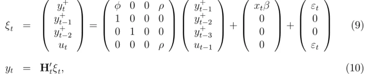
If we assume that the polynomial 1 1L pLp is of order one, i.e.,
p = 1, with coe¢cient , the state-space form of Möch and Uhlig’s problem is the
following: t = 0 B B @
y+t y+t 1 y+t 2
ut 1 C C A= 0 B B @ 0 0 1 0 0 0 0 1 0 0 0 0 0
1 C C A 0 B B @
yt+1 yt+2 yt+3
ut 1
1 C C A+ 0 B B @ xt 0 0 0 1 C C A+ 0 B B @ "t 0 0 "t 1 C C A (9)
yt = H0t t, (10)
where (9) and (10) are respectively the state and the observation equations and the matrix H0t is time-varying, with the following format:
H0t = 8 < :
1 1 1 0 ,t = 3;6;9;12; : : :
0 0 0 0 , otherwise.
(11)
One interesting feature of the approach in Mönch and Uhlig is that it encompasses several data interpolation models that are state-space based, summarized in Table 1 below:
Table 1 – Resulting Model as a Function of and in (9) Model
Static model in levels with IID residuals 0 0
Static model in levels with AR(1) residuals (Chow and Lin, 1971) 0 free Static model in 1st di¤erences with IID residuals (Fernandez, 1971) 0 1 Dynamic model in levels with IID residuals (Mitchell et al., 2005) free 0 Dynamic model in 1st di¤erences with IID residuals free 1 Dynamic model in levels with AR(1) residuals free free To assess the quality of interpolation, Mönch and Uhlig follow Bernanke, Gertler, and Watson (1997) by using twoR2 measures of …t. Denoting byyd+
estimate of monthly GDP, and by udtjT the same estimate of the error term ut, they
consider:
R2level = VAR d
y+tjT
VAR yd+tjT +VAR udtjT
, and,
R2di¤ = VAR
\y+
tjT
VAR \yt+jT +VAR \utjT
:
They claim it is more informative to report theR2 in …rst di¤erences since the same
statistic in levels will always be close to unity.
We now adapt the state-space representation in (9) and (10) to the problem of back-casting a series which we observe part of its realizations but not all. In some sense, this is very close to the problem worked out in Mönch and Uhlig, since they only observe quarterly GDP for some but not all months of the year. Their solution was to set to zero the missing observations. This seems like a clever and natural solution. It shuts down the missing values of the observed quarterly series in monthly frequency that are used in forecasting the state variable. This same principle is applied here to construct back-cast estimates of employment and income for the Brazilian economy.
Suppose we posses a total oft= 1;2; ; T ; ; T, observations onxt. However,
for series yt+, we only posses data fromt =T + 1; ; T, with missing values from
t= 1;2; ; T . This is exactly our setup for income and employment in this paper.
If we set the order of the polynomial 1 1L pLp to unity, i.e.,p= 1, with
coe¢cient , recalling that now we need not impose the time-aggregation restriction in (11), the state-space form of our problem collapses to the following:
t =
yt+
ut = 0
y+t 1 ut 1 +
xt
0 +
"t
"t (12)
yt = H0t t, (13)
where (12) and (13) are respectively the state and the observation equations and the matrix H0t is time-varying, with the following format:
H0t = 8 < :
1 0 , t=T + 1; ; T
0 0 , otherwise.
The key to the problem lies in the choice for H0t in (14). Here, we make the
latent variableyt+ identical toytfor the periods in which the latter is observed, with
no error term. This has two consequences. First, the algorithm will forecast yt+ to
be identical to yt for t = T + 1; ; T. Second, it will use the available data on
employment (income) to estimate a model and will use this model to forecast the latent variable in the periods in which it is not observable, i.e., fromt= 1;2; ; T .
Under correct speci…cation, this model can produce the optimal forecasts of the latent variable consistent with all available future information. That will be simply given by the smoothed forecast of yt+, i.e., byyd+tjT.
4
Empirical Results
4.1
Data
An important part of this paper is the choice of the variables to be included in the coincident indicator. We follow the recent Brazilian experience: Duarte, Issler and Spacov (2004) and Spacov (2001). For output, labelled Yt, we use industrial
production, computed by IBGE, and available from 1980:1. There is not a long-span sales series in Brazil, we therefore follow Duarte, Issler and Spacov and use total Brazilian production of corrugated paper as a proxy for sales, labelled St, which
is computed by ABPO. Employment, labelled Nt, is given by the total number of
persons – 10 years old or older – that have a job. It is extracted from the Monthly Employment Survey computed by IBGE. Income is proxied by the labor income series, labelledIt, extracted from this sameSurvey.
The last two series – employment and income – are only available from 2003 on, because of a drastic redesign of theMonthly Employment Survey. Here, we back-cast these series using a state-space representation estimated using the kalman …lter.
4.2
The Coincident Series
As stressed above, one of the original contributions of this paper is to back-cast two of the coincident series for the Brazilian economy – income and employment. We used the techniques described in the previous section to back-cast them. In the current
Monthly Employment Survey, income is available from 2002:2 on, while employment is available from 2002:3 on.
framework described above – based on the algorithm by Mönch and Uhlig (2005). Our setup allows for several di¤erent dynamic models to be estimated, all described in Table 1, depending on di¤erent values for the parameters and .
We tested seven series as auxiliary regressors in the back-casting procedure, all available for the period 1980:1 to 2007:11. They are: industrial production, output in the process industry, corrugated paper production, car production, steel production, cement production, energy production, and the monthly real GDP series estimated by Issler and Notini (2008). The dependent variables and all co-variates entered in levels in the state space representation, which is estimated in all the six di¤erent versions described in Table 1. In addition to the co-variates listed above, our models also include eleven seasonal dummies. In Table 2, we present theR2
di¤ measure of …t
for each model described in Table1.
Table 2 – Employment and Income Resulting R2di¤for each Model
Model Employment Income
Static model in levels with IID residuals 0:4979 0:1134 Static model in levels withAR(1) residuals 0:4729 0:0425 Static model in 1st di¤erences with IID residuals 0:0072 0:0000 Dynamic model in levels with IID residuals 0:0597 0:0827 Dynamic model in 1st di¤erences with IID residuals 0:0000 0:0000 Dynamic model in levels withAR(1) residuals 0:0000 0:0048
Our …nal choice of auxiliary variables and models was as follows. For employment (in logarithms) we choose only the monthly GDP series and energy production (in logarithms) as co-variates. For income (in logarithms), we selected only the paper production series and cement production (in logarithms) as auxiliary variables. In both cases, the model with the highestR2
level andR2di¤ was the static model with i.i.d.
errors, where set the parameters and equal to zero.
All four coincident series used in this paper are plotted below, which includes the results of the back-casted series. All four series – Production(Yt), Sales(St), Income
(It)and Employment(Nt)– were seasonally adjusted using the X-12 procedure. For
income and employment, the shaded areas in the graphs below depict the actual sample in which we observe them.
1.76 1.80 1.84 1.88 1.92 1.96 2.00 2.04 2.08 2.12
Figure 2: Sales - In log and Seasonally Adjusted
4.6 4.7 4.8 4.9 5.0 5.1 5.2 5.3
Figure 3: Income - In log and Seasonally Adjusted
2.7 2.8 2.9 3.0 3.1 3.2
1980 1985 1990 1995 2000 2005
Figure 4: Employment - In log and Seasonally Adjusted
3.90 3.95 4.00 4.05 4.10 4.15 4.20 4.25
80 82 84 86 88 90 92 94 96 98 00 02 04 06
Shaded areas depicts the actual sample
All four coincident series were tested for unit roots. We used three di¤erent tests. On a preliminary basis, we used the Augmented Dickey-Fuller (ADF) test. Initial results were later examined in light of the results of the Phillips and Perron (1988) test and the stationarity test proposed by Kwiatkowski et al. (1992). All four coincident series showed signs of unit roots in testing and therefore were transformed into …rst di¤erences (logs) prior to combination into a composite index.
Table 3: Coincident Series - Unit Root Tests
Variable ADF Kwiatkowski et. al Phillips and Perron t-statistic p-value LM-statistic t-statistic p-value
Employment -0.62 0.86 2.13* -0.55 0.88
Ind. Production -0.49 0.89 1.78* -0.87 0.80
Sales -0.34 0.92 2.12* -0.76 0.82
Income -0.43 0.90 2.10* -0.75 0.83
Notes:(i) ADF and Phillips and Perron H0:series has a unit root; KwiatkowskiH0:series is
4.3
TCB’s Coincident Index –
T CB
CI
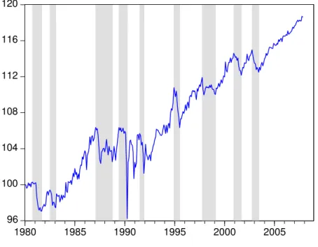
tUsing (1), we constructed a coincident index consistent with TCB’s method, labelled
T CB CIt, and plotted below. Next, we compare the turning-point dating of
this index with that of two other indices: a monthly estimate of Brazilian GDP computed by Issler and Notini (2008) and the composite index previously proposed by Duarte, Issler and Spacov (2004), available until 2002:11. The latter also uses TCB’s technique.
The turning points of these three composite indices were then compared using the Bry and Boschan (1971) and the Mönch and Uhlig (2005) dating algorithm, the latter being a slightly modi…ed version of the former. Results in Table 4 show that the current dating using TCB’s method yields results closer to the dating in Duarte, Issler and Spacov than to the dating of Brazilian monthly GDP. The most striking di¤erences appear in the dating of the 1991 recession. The dating of Duarte, Issler and Spacov and of GDP encompass two recession episodes into one as compared to the dating of T CB CIt. It is also noteworthy that GDP misses the two last
recessions as dated by T CB CIt and by Duarte, Issler and Spacov’s1.
1This behavior – GDP missing the last two recessions – vanishes if one uses the modi…ed
Figure 5: Coincident Index – Shaded Bry-Boschan Turning Points
96 100 104 108 112 116 120
1980 1985 1990 1995 2000 2005
Table 4 – Turning-Point Comparisons Using Bry-Boschan Dating
Peak Dates Through Dates
T CB CIt Duarte Brazilian T CB CIt Duarte Brazilian
et al. GDP et al. GDP
1980:10 NA 1981:09 NA 1981:11
1982:07 1982:6 1983:02 1983:10 1983:02
1987:02 1987:04 1988:3 1988:10 1989:02 1988:10 1989:06 1989:08 1989:6 1990:04
1991:07 1991:12 1991:03 1991:12
1994:12 1995:03 1994:12 1995:07 1995:09 1995:07 1997:10 1997:10 1997:10 1999:02 1999:02 1999:01
2000:12 2001:09
2002:10 2002:4 2003:06
Given the results in Table 4, we can compute how frequent Brazilian recessions are. From 1980-2007:11 we have a total of 9 recessions. On average, we observe in this period one recession at approximately every 3 years and 3 months, which is substantially more frequent than the U.S. historical average of one recession about every 5 years. Recessions in Brazil also last longer than U.S. recessions: while ours last about 12 months, on average, U.S. recessions last typically from 6 months to one year, on average (in our sample period here – 1980:1 to 2007:11 – U.S. recessions lasted, on average, 9 months). Indeed, Duarte, Issler and Spacov make the point that this behavior may be due to hardships that the Brazilian economy has endured in the post-1980 era, where GDP growth declined form about 7% a year in real terms prior to 1980 to about 2.2% a year after 1980.
Table 5 below lists Brazilian recessions from 1980:1 to 2007:11 when the dating of turning points is made using the modi…ed Bry and Boschan technique proposed by Mönch and Uhlig (2005). The latter takes into account asymmetry di¤erences in peak and through dating, which may be at work to explain the di¤erence in dating between the Bry and Boschan and the Mönch and Uhlig method. Here, the dating of peaks inT CB CIt is identical to that in Brazilian GDP, whereas the dating of
throughs is almost identical.
Table 5 – Turning-Point Comparisons Using Mönch and Uhlig Dating
Peak Dates Through Dates
T CB CIt Duarte Brazilian T CB CIt Duarte Brazilian
et al. GDP et al. GDP
1980:10 NA 1980:10 1981:09 NA 1981:11
1982:07 1982:07 1983:02 1983:02
1987:02 1987:04 1987:02 1988:10 1989:02 1988:10
1989:06 1989:08 1989:06 1990:04 1990:04
1991:07 1991:07 1991:12 1991:12 1991:12
1994:12 1994:12 1994:12 1995:07 1995:9 1995:07 1997:10 1997:10 1997:10 1999:02 1999:02 1999:01 2000:12 2000:12 2000:12 2001:09 2001:9 2001:09
2002:10 2002:10 2003:06 2003:03
Notes: The analysis in Duarte et al. (2004) starts in 1982:05, therefore could not have dated the recession of 1980. Brazilian GDP dating uses the monthly series constructed by Issler and Notini (2008).
generates a sensible composite coincident index of economic activity. The latter is able to approximate reasonably well the turning points of monthly GDP and those of the TCB index using the retired income and employment series in Duarte, Issler and Spacov (2004). Of course, there are more similarities in turning-point dating when dating uses the technique proposed by Mönch and Uhlig.
We believe that the strategy we chose in this paper to construct a long span time-series for the Brazilian coincident indicator was the best possible. An alternative would be to chain the current employment and income series with their respective series retired by IBGE. Since the redesign of the Monthly Employment Survey was drastic, this procedure would chain completely di¤erent series. Another alternative would be to only use industrial production and sales to construct the composite index up to 2002:2, and then use the four usual series from 2002:3 onwards. This procedure would probably induce structural changes in mean and variance of the composite index after 2002:3.
4.4
The Composite Leading Indicator
Leading indicators are widely used in predicting turning points of business cycles in many countries. The selection of a leading indicator index involves three steps: (i) select an appropriate indicator as a measure of economic activity to be targeted, also called a reference series; (ii) select appropriate economic and …nancial indicators as predictors of the turning points of the reference series; (iii) combine the selected leading series in order to construct a composite leading index.
The …rst step was accomplished in the previous section, where we obtained a composite index of economic activity for the Brazilian economy after we back-cast the employment and income series. The next step is to select appropriate leading in-dicators as predictors of turning points. We search for series that satisfy the following conditions: (a) to be observable at a monthly frequency for the period 1980-2007:11; (b) timely data releases, and having small revisions regarding …nal data …gures.
From FGV’s survey series and other Brazilian databases (IBGE, IPEADATA, and the Central Bank’s), we selected 44 series that are candidates of being leading series of the coincident index. Our choice was guided by the international experience (Stock and Watson (1989, 1993)) and also by local experience (Duarte, Issler and Spacov (2004)).
A main issue regarding FGV’s survey series is that they were computed on a quar-terly frequency up to September 2005. From then on, surveys were then conducted on a monthly basis. Therefore, there is the need to interpolate the data on quarterly frequency to have an homogeneous series on a monthly basis. Our interpolation method was, again, Mönch and Uhlig’s (2005).
All leading nominal series were de‡ated to re‡ect their purchasing power as of March, 2008. The de‡ator used was the Brazilian General Price Index “IGP-DI” – calculated by FGV. All series denominated in foreign currency were converted into Brazilian Reais at the prevailing exchange rate and subsequently de‡ated. All series were logged, unless logs could not be taken of the original series (potentially zero or negative …gures). All series were also seasonally adjusted prior to the analysis using the X-12 procedure, whenever a seasonal pattern in them was detected.
With the exception of the survey-tendency series, all leading series were tested for unit roots. Survey series are bounded series, by construction. Therefore, they cannot posses a unit root, which leads to unbounded series in theory. To test for unit roots we used the Augmented Dickey-Fuller (ADF) test, the Phillips and Perron (1988) test, and the stationarity test proposed by Kwiatkowski et al. (1992). All series with a unit root were transformed into …rst di¤erences (logs) prior to combination into a composite index2.
In order to measure the quality with which a leading series correctly anticipates the “state of the economy” implied by the coincident series (recession or expansion), we use a criterion originally proposed by Diebold and Rudebusch (1999), and later employed by Zhang and Zhuang (2002) and Gallardo and Pedersen (1997). The Quadratic Probability Score, labelled as QP S(h), is given by:
QP S(h) =
T
X
t=1
(Pt Rt)2
T (15)
where Pt denotes the predicted state outcomes from a candidate leading indicator
andRtdenotes the observed realizations of the reference series. Both are equal to one 2ADF unit-root test results are presented in Table A3 in the Appendix. Other test results are
for a turning point and zero otherwise;T is the total number of sample observations,
while h is the horizon in which the leading series potentially predicts the reference
series. By construction, the value ofQP S(h)ranges between zero and one, with zero indicating a perfect …t for the the “state of the economy” of the reference series.
Next, we describe the basic criteria used to select the leading series that will compose our index. First, for each series, we calculate the optimum (minimum)
QP S(h) value, denoted by QP S(h ), where h is the resulting optimum lag. To be
a leading series candidate, the series must have h > 0 in QP S(h ). This means
that the series is leading, not lagging or coincident to reference series. Second, we apply Granger (1969) causality tests in order to examine whether the leading series precedes the reference series. We expect that a leading series Granger-causes the reference series but is not Granger-caused by it.
In the Appendix, Table A4 shows the QP S(h ), h , and Granger-causality test
results. The majority of the potential leading series do not Granger cause the coin-cident series. The exceptions are some FGV’s survey series, in addition to SELIC – Central Bank’s basic interest rate – and IBOVESPA – Brazilian Stock Market Index. From them, IBOVESPA shows promise, since its QP S(h ) = 24:5%, and h = 5. This means that, when we take the IBOVESPA index, with a lag of 5 months vis-à-vis period t, it correctly predicts 24:5% of the “state of the economy” as measured by the peak and though behavior of our our composite index. A slightly worse result in observed to the survey series on the production of real-estate inputs –QP S(h ) = 25:1%, and h = 1.
The QP S( ) statistic has only three series with values between 10 and 20% – intermediate-good production, consumer-good production, and inventories, and a few between20and30%. The intersection of the two criteria above – “Granger causality” and “low QP S(h )” – only has the IBOVESPA index and the production of
real-estate inputs. Across all potential leading series the mean lag is 3, but the median and modal lag are 1. There are several interesting series which have h > 1 and a relatively low QP S(h ): FGV’s survey series on inventories (QP S(h ) = 17:6%),
the IBOVESPA index (QP S(h ) = 24:5%), as well as a myriad of other FGV’s
survey series.
Looking at results in Table A4, there is no obvious way to select series to be in the composite index. We present next 10 ad-hoc criteria to select those series, the idea being that we wanth to be high, QP S(h ) to be low, and that a leading series Granger-causes the reference series but is not Granger-caused by it. We also investigate whether a series that has low h , with low QP S(h ), would also have a
relatively lowQP S(h) for higher values of h. The 10criteria are listed below:
2. Select all series possessing QP S(h) less than 0:4;
3. Select all series that satis…ed the Granger causality test criterion;
4. Select all series in the intersection between the …rst and third criterion;
5. Select all series in the intersection between the second and third criterion;
6. Select all Survey series that satis…ed the Granger causality test criterion;
7. Select the …ve series in Table A4 that have the lowest QP S(h)value;
8. Select the series for which h is between two and seven months and QP S(h )<
0:3;
9. Select the series for which h is between two and seven months;
10. Select survey series for which QP S(h )<0:3.
Given these criteria, we computed 10 di¤erent composite leading indices of eco-nomic activity, labelled LIi;t, i = 1;2; ;10. We chose to combine leading series
into the composite index using a counterpart of equation (1) – equal weights on standardized growth rates of the leading series3.
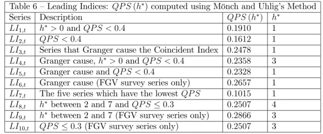
Table 6, below, lists the values ofQP S for each criterion listed above, computed
for the optimum lag, i.e., QP S(h ).
Table 6 – Leading Indices: QP S(h )computed using Mönch and Uhlig’s Method
Series Description QP S(h ) h
LI1;t h >0and QP S <0:4 0:1910 1
LI2;t QP S <0:4 0:1612 1
LI3;t Series that Granger cause the Coincident Index 0:2478 1
LI4;t Granger cause, h >0 and QP S <0:4 0:2358 3
LI5;t Granger cause andQP S <0:4 0:2328 1
LI6;t Granger cause (FGV survey series only) 0:2657 1
LI7;t The …ve series which have the lowest QP S 0:1015 1
LI8;t h between 2 and 7 andQP S 0:3 0:2507 4
LI9;t h between 2 and 7 (FGV survey series only) 0:2866 3
LI10;t QP S 0:3 (FGV survey series only) 0:2507 3
3Tables A5 and A6 in Appendix compare the turning points data for each leading index and the
From the results in Table 6 LI7;t stands out as a candidate of composite
in-dex. The leading series in it have their QP S(h ) between 11:04% and 23:28%.
Despite that, the composite index has aQP S(h ) = 10:15%– lower than the small-est QP S(h ) of the series in it. The latter are all Industry Survey series: of the Consumer-Good Industry, Capital-Good, Real-Estate Input, Intermediary-Good and the Level of External Demand. The composite indicesLI2;t and LI1;t also do well in
terms of QP S(h ) and can be considered as an alternative toLI7;t.
Our next exercise is a dating exercise involving T CB CIt and LIi;t, i =
1;2; ;10. We want to examine how well and how often these leading indices
predict the turning points inT CB CIt. We are also interested in knowing whether
they generate false predictions, i.e., predicting a non-existent peak or through in eco-nomic activity. We start with a 24-month window around period /t, i.e., from /t 12 through /t+12, and consider turning points inT CB CItand inLIi;t,i= 1;2; ;10.
From peak and through dates inT CB CIt and LIi;t, we are able to match peaks
of T CB CIt with peaks of LIi;t, and throughs of T CB CIt with throughs of
LIi;t. We can also compute the average lead in peak (or through) prediction for each
episode, as well as to list false predictions of turning points.
Results of this exercise are presented in Tables 7 through 11 for LI7;t, LI2;t and
LI1;t. The Appendix contains this exercise for the remaining leading indices.
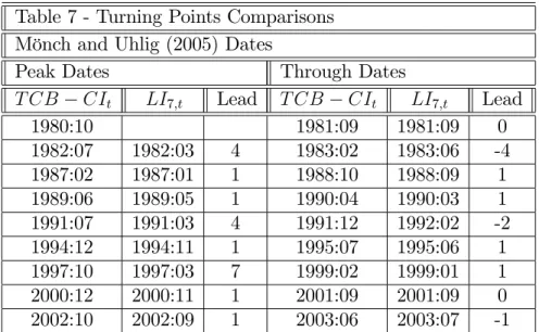
Table 7 shows respectively the coincident index andLI7;tpeaks and through dates.
Peak prediction is much better done than through prediction: only one peak is lost and LI7;t anticipates the coincident-index peaks 2.5 months ahead, on average. For
throughs, although none is lost, on three occasions through prediction ofLI7;t occurs
Table 7 - Turning Points Comparisons Mönch and Uhlig (2005) Dates
Peak Dates Through Dates
T CB CIt LI7;t Lead T CB CIt LI7;t Lead
1980:10 1981:09 1981:09 0
1982:07 1982:03 4 1983:02 1983:06 -4 1987:02 1987:01 1 1988:10 1988:09 1 1989:06 1989:05 1 1990:04 1990:03 1 1991:07 1991:03 4 1991:12 1992:02 -2 1994:12 1994:11 1 1995:07 1995:06 1 1997:10 1997:03 7 1999:02 1999:01 1 2000:12 2000:11 1 2001:09 2001:09 0 2002:10 2002:09 1 2003:06 2003:07 -1
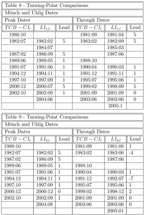
Table 8 performs the same analysis above forLI1;t. The average lead for for peak
prediction is again 2:5 months, while that for through prediction is 2:25 months. However,LI1;tpredicts two extra peaks and three extra throughs than those observed
onT CB CIt. This result is in contrast with that ofLI7;t, which predicted no extra
peaks or throughs.
For LI2;t the results in Table 9 show an average lead for peak prediction of 1:88
months, with a lead of 0:75 months for through prediction, a very bad result for through prediction. Moreover,LI2;t predicts one extra peak and two extra throughs
than those observed on T CB CIt. This result is in contrast with that of LI7;t,
which predicted no extra peaks or throughs.
Focusing on the overall results for turning-point prediction only, it is clear that
LI7;tdominates eitherLI1;torLI2;t: all three missed one peak, butLI7;t predicted no
extra peaks, whileLI2;t predicted two extra peaks andLI2;tpredicted one. Regarding
throughs, all three composite indices did not miss any, while LI7;t predicted no
extra throughs, which contrasts with the results forLI1;t and LI2;t: three and two,
Table 8 - Turning-Point Comparisons Mönch and Uhlig Dates
Peak Dates Through Dates
T CB CIt LI1;t Lead T CB CIt LI1;t Lead
1980:10 1981:09 1981:04 5
1982:07 1982:02 5 1983:02 1982:09 5
1984:07 1985:03
1987:02 1986:09 5 1987:06
1989:06 1989:05 1 1988:10
1991:07 1991:06 1 1990:04 1990:03 1 1994:12 1994:11 1 1991:12 1991:11 1 1997:10 1997:09 1 1995:07 1995:06 1 2000:12 2000:07 5 1999:02 1998:09 5 2002:10 2002:09 1 2001:09 2001:09 0
2004:06 2003:06 2003:06 0
2005:1
Table 9 - Turning-Point Comparisons Mönch and Uhlig Dates
Peak Dates Through Dates
T CB CIt LI2;t Lead T CB CIt LI2;t Lead
1980:10 1981:09 1981:08 1
1982:07 1982:02 5 1983:02 1983:06 -4
1987:02 1986:09 5 1987:06
1989:06 1989:05 1 1988:10
1991:07 1991:06 1 1990:04 1990:03 1 1994:12 1994:11 1 1991:12 1992:07 -7 1997:10 1997:09 1 1995:07 1995:06 1 2000:12 2000:12 0 1999:02 1998:12 2 2002:10 2002:09 1 2001:09 2001:09 0
2004:08 2003:06 2003:06 0
2005:01
Tables 10 and 11 contain, respectively, peak and through dating statistics for all 10 composite leading indices. It becomes clear that the good QP S( ) statistic for
extra peaks and throughs vis-à-vis alternative indices.
All and all, considering the whole evidence in this section, we choose LI7;t to be
our composite leading index of economic activity. Our choice is supported by aQP S
value of 10:15%, meaning that this leading index provides wrong predictions of the
state of the Brazilian economy only in10:15% of the time.
There is a somewhat asymmetric behavior forLI7;t in terms of peak and through
prediction: on average, whileLI7;t predicts peaks with a two-and-a-half-month lead,
it predicts throughs with a very small average lead of 0:37months. Because of this behavior, we might want to consider either LI1;t as an alternative composite index
for the purpose of through prediction only, since it leadsT CB CItby2:25months.
Table 10 - Leading Indices: Peak Dating Comparisons Mönch and Uhlig Dates
Index # of Peaks # LeadingPeaks # MissedPeaks # ExtraPeaks
T CB CIt 9 - -
-LI1;t 10 8 1 2
LI2;t 9 8 1 1
LI3;t 7 6 3 1
LI4;t 10 7 2 3
LI5;t 8 6 3 2
LI6;t 8 6 3 2
LI7;t 8 8 1 0
LI8;t 8 8 1 0
LI9;t 10 7 2 3
Table 11 - Leading Indices: Through Dating Comparisons Mönch and Uhlig Dates
Index # of Throughs # LeadingThroughs # MissedThroughs # ExtraThroughs
T CB CIt 9 - -
-LI1;t 11 8 1 3
LI2;t 10 8 1 2
LI3;t 8 7 2 1
LI4;t 11 9 0 2
LI5;t 9 7 2 2
LI6;t 8 6 3 2
LI7;t 9 9 0 0
LI8;t 10 8 1 2
LI9;t 11 8 1 3
LI10;t 10 8 1 2
Finally, in the Figure below, we plotT CB CItandLI7;t smoothed by computing
a three-month moving average. They have a straking similar behavior for the sample period covered in this paper. Of course, the originalLI7;tleads the originalT CB CIt
Figure 6: Coincident and Leading Indexes
96 98 100 102 104 106 108 110
96 100 104 108 112 116 120 124
80 82 84 86 88 90 92 94 96 98 00 02 04 06 08
Leading Index - Criterium 7 (MA3) Coincident Index (MA3)
5
Conclusion
Once we obtained a long enough span of the usual series used in TCB’s method, we compute a new composite coincident index of Brazilian economic activity. Its dating of recessions is compared with those in Duarte, Issler and Spacov and with those implied by the monthly GDP estimate computed by Issler and Notini (2008).
Our last contribution is to propose a composite leading index of economic activity to track our composite coincident index. This is an important topic here, since Brazilian research had focused mainly on the construction of coincident indices. After a wide empirical search, we settled for a composite index that predicts correctly the “state of the economy” (expansion vs. recession), measured by our coincident index, almost 90% of the time. It misses one peak in economic activity and no through, while predicting no extra peaks or throughs. Moreover, on average, it leads the coincident index by 2:5 months for peaks and by 0:33 months for throughs. For anticipating throughs alone, an alternative composite leading index increases this lead to2:25months.
Finally, it is worth stressing that our choice of leading composite index – LI7;t
– uses only series contained in the survey of industrial activity conducted by FGV: Consumer-Good activity, Capital-Good activity, Real-Estate Input activity, Intermediary-Good activity and the Level of External Demand. Since the criterion to choose the series in LI7;t was based solely on the …ve best values for QP S( ), it is interesting
to …nd that only survey series made the top-…ve spots on that list.
References
[1] Bernanke, Ben, Gertler, Mark, and Mark Watson (1997): “Systematic Monetary Policy and the E¤ects of Oil Price Shocks”, Brookings Papers on Economic Activity, 1997(1), 91-157.
[2] Boehm, E. and Moore, G. H. (1984). “New Economic Indicators for Australia”,
The Australian Economic Review, 4th quarter, 34-59.
[3] Bry, G. and Boschan, C. (1971). “Cyclical Analysis of Time Series: Selected Procedures and Computer Programs.” New York: National Bureau of Economic
Research.
[5] Chauvet, M. (1998). “An Econometric Characterization of Business Cycle Dy-namics with Factor Structure and Regime Switching”, International Economic Review, 39, 969-996.
[6] Chauvet, M. (2001). “A Monthly Indicator of Brazilian PIB”, Brazilian Review of Econometrics, 21, 1-48.
[7] Chauvet, M. (2002). “The Brazilian Business Cycle and Growth Cycles”,Revista Brasileira de Economia, 56, 75-106.
[8] Chow, Gregory C., and An-loh Lin (1971): “Best Linear Unbiased Interpolation, Distribution, and Extrapolation of Time Series by Related Series”,The Review of Economics and Statistics, 53(4), 372-375.
[9] Contador, R. C. (1977). “Ciclos Econômicos e Indicadores de Atividade.” Rio
de Janeiro, INPES/IPEA, 237 p.
[10] Contador, C. and Ferraz, C. (1999). “Previsão com Indicadores Antecedentes.”
Rio de Janeiro: Silcon.
[11] Cuche, N. A. and Hess, M. K. (2000) Estimating monthly GDP in a general Kalman …lter framework: evidence from Switzerland. Economic and Financial Modelling, v. 7, n. 4, p. 153-194.
[12] Diebold F.X., and Rudebusch, G.D. (1989). Scoring the leading indicators, The Journal of Business, Vol. 62, No. 3, pp. 596-616, July.
[13] Diebold F.X., and Rudebusch, G.D. (1990). A Nonparametric Investigation of Duration Dependence in the American Business Cycle, The Journal of Political Economy, Vol. 98, No. 3, (June, 1990), pp. 596-616.
[14] Duarte, A. J. M.; Issler J. V.; Spacov A., “Coincident Indices of Economic Activity and a Chronology of Brazilian Recessions,” (in Portuguese), Pesquisa e Planejamento Econômico, v. 34(1), pp. 1-37, 2004.
[15] Engle, R. F. and Granger, C. (1987). “Cointegration and Error Correction: Representation, Estimation and Testing”,Econometrica, 55, 251-276.
[17] Fernandez, Roque (1981): “A Methodological Note on the Estimation of Time Series”,Review of Economics and Statistics, 63, 471-478.
[18] Forni, M., Hallin, M., Lippi, M. and Reichlin, L. (2000), “The Generalized Dynamic Factor Model: Identi…cation and Estimation”, Review of Economics and Statistics, 2000, vol. 82, issue 4, pp. 540-554.
[19] Gallardo, M. and Pedersen, M., (2007). Indicadores líderes compuestos. Re-sumen de metodologias de referencia para construir um indicador regional em América Latina. Serie Estúdios estadísticos y prospectivos, CEPAL, 2007.
[20] Hamilton, J. D. (1989). “A New Approach to The Economic Analysis of Non-stationary Time Series and The Business Cycle”,Econometrica, 57, 357-384.
[21] Hamilton, J. D. (1994). “Time Series Analysis,” Princeton University Press. [22] Harding, D. and Pagan, A. (2002b). “Dissecting the Cycle: A Methodological
Investigation”, Journal of Monetary Economics, 49, 365-81.
[23] Harvey, A. (1989). Forecasting, Structural Time Series and the Kalman Filter, Cambridge: Cambridge University Press.
[24] Harvey, A. C. and Pierse, R. G. (1984). ‘Estimating missing observations in economic time series’, Journal of the American Statistical Association, vol. 79, pp. 125–31.
[25] Hollauer, G.; Issler, J.; and Notini, H. (2008). "Novo Indicador Coincidente para a Atividade Industrial Brasileira",Graduate School of Economics, Getulio Vargas Foundation. Forthcoming Brazilian Journal of Applied Economics.
[26] Issler, J.V. and Notini, H.H., 2008, “Estimating Brazilian Monthly Real PIB: a Kalman Filter Approach,” paper submitted to CIRET 2008, mimeo., Graduate School of Economics, Getulio Vargas Foundation.
[27] Issler, J.V. and Spacov, A. D. (2000). “Usando Correlações Canônicas para Identi…car Indicadores Antecedentes e Coincidentes da Atividade Econômica no Brasil”, mimeo, Relatório de Pesquisa para o Ministério da Fazenda.
[28] Issler, J. V., Vahid, F., 2005, “The missing link: “Using the NBER recession indicator to construct coincident and leading indices of economic activity,” Jour-nal of Econometrics, Annals Issue on “Common Features,” vol. 132, no. 1, pp.
[29] Kwiatkowski, D., P.C.B. Phillips, P. Schmidt e Y. Shin (1992), “Testing the Null Hypothesis of Stationarity Against the Alternative of a Unit Root: How Sure Are We That Economic Time Series Have a Unit Root?” Journal of Econometrics, vol. 54, pp. 159-178.
[30] Lucas, R. E. Jr. (1977). “Understanding Business Cycles”, Carnegie-Rochester Conference Series on Public Policy, 5, 7-29.
[31] Mariano, R. e Murasawa, Y. (2003). “A New Coincident Index of Business Cycles Based on Monthly and Quarterly Series,”Journal of Applied Econometrics, 18, 427-43.
[32] Mitchell, James, Richard J. Smith, Martin R. Weale, Stephen Wright, and Ed-uardo L. Salazar (2005): “An Indicator of Monthly PIB and an Early Estimate of Quarterly PIB Growth”,The Economic Journal, 115, F108-F129.
[33] Monch, E. and Uhlig, H. (2005). "Towards a Monthly Business Cycle Chronology for the Euro Area". Journal of Business Cycle Measurement and Analysis 2(1).
[34] Newey, W. and West, Kenneth (1987) “A Simple Positive Semi-De…nite, Het-eroskedasticity and Autocorrelation Consistent Covariance Matrix”, Economet-rica, 55, 703-708.
[35] Phillips, P. and Perron, P. (1988) “Testing for a Unit Root in Time Series Regression.” Biometrika, vol. 75, pp. 335-46.
[36] Picchetti, P and Toledo, C. (2002). “Estimating and Interpreting a Common Stochastic Component for the Brazilian Industrial Production Index”, Revista Brasileira de Economia, 56, 107-20.
[37] Reichlin, L. (2000). “Extracting Business Cycle Indexes from Large Data Sets: Aggregation, Estimation, Identi…cation”, in Dewatripont, M., Lars, P. e Turnowski (Ed.),Advances in Economics and Econometrics, Cambridge
Uni-versity Press.
[38] Rivers, D. and Vuong, Q. (1988). “Limited Information Estimators and Exo-geneity Tests for Simultaneous Probit Models”, Journal of Econometrics, 39,
347-366.
[40] Stock, J. and Watson, M. (1988a). “A New Approach to Leading Economic Indicators”, mimeo, Harvard University, Kennedy School of Government.
[41] Stock, J. and Watson, M. (1988b). “A Probability Model of The Coincident Economic Indicators”, NBER Working Paper no 2772.
[42] Stock, J. and Watson, M. (1989). “New Indexes of Coincident and Leading Economics Indicators”,NBER Macroeconomics Annual, 351-95.
[43] Stock, J. and Watson, M. (1993a). “A Procedure for Predicting Recessions with Leading Indicators: Econometric Issues and Recent Experience”, in New Re-search on Business Cycles, Indicators and Forecasting, J. Stock e M. Watson, Eds., Chicago: University of Chicago Press.
[44] Stock, J. and Watson, M. (1993b).New Research on Business Cycles, Indicators and Forecasting, J. Stock e M. Watson, Eds., Chicago: University of Chicago Press.
[45] Vahid, Farshid and Engle, R. F. (1993). “Common Trends and Common Cycles”,
Journal of Applied Econometrics, 8, 341-360.
[46] Vahid, Farshid and Issler, J. V. (2002). “The Importance of Common-Cyclical Features in VAR Analysis: A Monte-Carlo Study”, Journal of Econometric,
109, 341-363.
6
Apendix
6.1
The Bry and Boschan (1971) Algorithm
BRY BOSCHAN PROCEDURE FOR PROGRAMMED DETERMINA-TION OF TURNING POINTS
I. Determination of extremes and substitution of values
II Determination of cycles in 12-month moving average (extremes replaced) A. Identi…cation of points higher (or lower) than 5 months on either side
B. Enforcement of alternation of turns by selecting highest of multiple peaked (or lowest of multiple troughs).
III Determination of corresponding turns in Spencer curve (extremes replaced). A. Identi…cation of highest (or lowest) value within 5 months of selected turn in 12-month moving average.
B. Enforcement of minimum cycle duration of 15 months by eliminating low-erpeaks and higher troughs of shorter cycles
IV Determination of corresponding turns in short- term moving average of 3 to 6 months, depending on MCD (months of cyclical dominance).
A. Identi…cation of highest (or lowest) value within 5 months of selected turn in Spencer curve.
V. Determination of turning points in unsmoothed series
A. Identi…cation of highest (or lowest) value within 4 months, or MCD term, whichever is larger, of selected turn in short-term moving average.
B. Elimination of turns within 6 months of beginning and end of series.
C. Elimination of peaks (or troughs) at both ends of series which are lower (or higher) than values closer to end.
D. Elimination of cycles whose duration is less than 15 months. E. Elimination of phases whose duration is less than 5 months. VI. Statement of …nal turning points.
Source: Bry and Boschan (1971) page 21.
Table A1: Leading Series
Series name Description Source
BASE_R Monetary base Bacen
SELIC_R Selic interest rate Bacen
M1_R M1 money stock Bacen
IBOV_R Ibovespa index Bovespa
EXP_PRECOS Exports prices Funcex
EXP_QUANTUM Quantum of exports Funcex
EXP_R Exports (FOB) Funcex
TTROCA Terms of trade Funcex
IMP_PRECOS Imports prices Funcex
IMP_QUANTUM Quantum of imports Funcex
IMP_R Imports (FOB) Funcex
CAMBIO_R Exchange Rate Bacen
NUCIFIESP Manufacturing Industry Fiesp
PROD_BC Production - Consumer Goods IBGE/PIM
PROD_BCD Production - Consumer Durable IBGE/PIM
PROD_BCND Production - Consumption and Non Durable IBGE/PIM
PROD_BI Production - Intermediate Goods IBGE/PIM
PROD_BK Production - Capital Goods IBGE/PIM
PRODINDT Industrial production - processing industry IBGE/PIM
PRODONI Production - bus IBGE/PIM
PRODVEI Production - vehicles Anfavea
PRODAUTO Production - motors Anfavea
PRODCAM Production - trucks Anfavea
SAL_R Nominal Salary - industry
PO Sta¤ employed - industry Fiesp
HPP Hours paid - industry Fiesp
HTP Hours worked in production - industry Fiesp
ICMS_R Confaz
INPC_R National Consumer Price Index
SPC ACSP
IPA_R FGV
Table A2: Survey Leading Series
Business Tendency Survey Description Source
NUCI_BR Survey of Manufacturing Industry FGV
NUCI_BC Survey of Consumer Goods Industry FGV
NUCI_BK Survey of Capital Goods Industry FGV
Table A3: Leading Series - ADF Unit Root Test
Series t-statistic p-value
BASE_R -2.89 0.17
CAMBIO_R -1.83 0.69
DEMGLOB -2.92 0.16
DEMPREV -4.42 0.00*
EMPPREV -2.72 0.23
ESTOQUES -5.06 0.00*
EXP_PRECOS -0.16 0.99
EXP_QUANTUM -2.71 0.23
EXP_R -1.85 0.68
FALENCIAS -2.38 0.39
HPP -1.85 0.68
HTP -1.99 0.61
IBOV_R -3.45 0.04*
ICMS_R -5.53 0.00*
IMP_PRECOS -0.77 0.97
IMP_QUANTUM -2.91 0.16
IMP_R -2.61 0.28
INPC_R -1.68 0.00*
IPA_R -1.08 0.93
M1_R -2.15 0.52
NUCI_BR -3.46 0.04*
NUCIFIESP -5.20 0.00*
PO -1.11 0.92
PROD_BC -2.96 0.14
PROD_BCD -3.52 0.04*
PROD_BCND -2.96 0.15
PROD_BI -2.28 0.44
PROD_BK -3.10 0.11
PRODCAM -5.23 0.00* PRODINDT -2.54 0.31 PRODONI -1.11 0.00* PRODPREV -3.29 0.07 PRODVEI -7.12 0.00*
SAL_R -3.44 0.04*
SELIC_R -1.45 0.00*
SPC -2.16 0.51
TTROCA -4.28 0.00*
NUCI_BC -2.40 0.14
NUCI_MC -2.16 0.22
NUCI_BI -2.88 0.04*
DeMINT -3.04 0.03*
DEMEX -5.24 0.00*
DEMPREVINT -3.84 0.00* DEMPREVEXT -3.40 0.01*
Notes: (i) the speci…cation of the test equation was chosen on the basis of the Schwartz Information Criterion; (ii) the asterisk (*) indicates that we reject the null hypothesis of
Table A4: Leading Series - QP S(h ) and Granger Causality
Leading Optimum h Mín QPS-QP S(h ) Granger-Causes
BASE_R 1 0.4567 B
DEMGLOB 3 0.2806 B
DEMPREV 4 0.2866 B
EXP_R 7 0.3642 N
EXP_QUANTUM 12 0.3104 N
HPP 1 0.4299 B
HTP 1 0.3940 N
IMP_R 1 0.3761 N
IPA_R 11 0.5164 N
M1_R 1 0.3373 C
NUCI_BC 1 0.3463 C
NUCI_BK 1 0.3134 C
NUCI_MC 1 0.2507 C
PO 1 0.4090 N
PRODAUTO 1 0.2149 B
PROD_BC 1 0.1254 B
PROD_BCND 1 0.2328 N
PROD_BI 1 0.1104 N
PROD_BK 1 0.3463 N
PRODINDT 1 0.3104 N
ESTOQUES 2 0.1761 B
IBOV_R 5 0.2448 C
ICMS_R 1 0.3134 B
INPC_R 5 0.4776 N
NUCI_BR 1 0.2746 B
NUCIFIESP 1 0.2478 B
PROD_BCD 1 0.2746 N
PROD_CAM 1 0.2627 N
PRODONI 1 0.4179 N
of lags tested was set at 3, 6, 12. To compute the results of the Granger test it was considered the existence of causality in at least one of these lags.
Table A4 (continuation)
Leading Optimum h Mín QPS-QP S(h ) Granger-Causes
PRODPREV 3 0.2507 N
PRODVEI 1 0.3224 N
SAL_R 1 0.3761 N
NUCI_BI 1 0.3224 B
CAMBIO_R 12 0.6000 B
EXP_PRECOS 3 0.3881 N
IMP_PRECOS 10 0.5045 N
SELIC_R 11 0.5821 C
TTROCA 2 0.3642 N
DEMEXT 6 0.3164 N
DEMINT 2 0.2746 B
DEMPREVEXT 4 0.3463 N
DEMPREVINT 4 0.2716 B
IMP_QUANTUM 1 0.3343 N
LN_SPC 1 0.2537 B
Table A5: Leading Indices - Mönch e Uhlig Dates
Table A5 – Selected Leading Index
Turning Points Comparatives– Mönch e Uhlig
Peak dates Through dates
TCB - CI LI3 Lag TCB - CI LI3 Lag
1980:10 1981:09
1982:07 1983:02 1983:06 +4
1987:02 1986:09 -5
1989:06 1989:03 -3 1988:10 1988:12 +2 1991:07 1991:04 -3 1990:04 1990:03 -1 1994:12 1994:11 -1 1991:12 1992:07 +7 1997:10 1997:08 -2 1995:07 1995:09 +2 2000:12 2001:03 +3 1999:02 1998:11 -3
2002:10 2001:09 2002:03 +6
2004:09 2003:06
2005:12
Table A5 – Selected Leading Index (continuation) Turning Points Comparatives– Mönch e Uhlig
Peak dates Through dates
TCB - CI LI4 Lag TCB - CI LI4 Lag
1980:10 1981:09 1981:03 -6
1982:07 1981:11 -8 1983:02 1982:10 -4
1984:04 1985:03
1987:02 1986:09 -5 1988:10 1988:07 -3 1989:06 1989 3 -3 1990:04 1990:02 -2
1990:06
1991:07 1991:12 1992:12 +12
1994:12 1994:09 -3 1995:07 1995:07 0 1997:10 1997:06 -4 1999:02 1998:11 -3 2000:12 2000:12 0 2001:09 2001:09 0 2002:10 2002:09 -1 2003:06 2003:01 -5
Table A5 – Selected Leading Index (continuation) Turning Points Comparatives– Mönch e Uhlig
Peak dates Through dates
TCB - CI LI6 Lag TCB - CI LI6 Lag
1980:10 1981:09
1982:07 1982:04 -3 1983:02 1983:06 +4 1987:06 1987:02 1986:09 -5 1988:10
1988:03
1989:06 1990:04 1990:03 -1
1991:07 1991:04 -3 1991:12 1992:06 +6 1994:12 1994:12 0 1995:07 1995:09 +2 1997:10 1997:06 -4 1999:02 1998:12 -2 2000:12 2000:12 0 2001:09
2002:10 2003:06 2002:06 -12
2004:09 2005:12
Table A5 – Selected Leading Index (continuation) Turning Points Comparatives– Mönch e Uhlig
Peak dates Through dates
TCB - CI LI8 Lag TCB - CI LI8 Lag
1980:10 1981:09 1981:04 -5
1982:07 1982:04 -3 1983:02 1983:07 +5 1987:7 1987:02 1986:07 -7 1988:10
1989:06 1989:04 -2 1990:04 1990:04 0 1991:07 1991:07 0 1991:12 1991:10 -2 1994:12 1994:10 -2 1995:07 1995:07 0 1997:10 1996:10 -12 1999:02 1998:10 -4 2000:12 2000:07 -5 2001:09 2001:07 -2 2002:10 2002:01 -9 2003:06 2003:07 +1
Table A5 – Selected Leading Index (continuation) Turning Points Comparatives– Mönch e Uhlig
Peak dates Through dates
TCB - CI LI9 Lag TCB - CI LI9 Lag
1980:10 1981:09 1981:04 -5
1982:07 1982:01 -6 1983:02 1982:10 -4 1985:03
1984:04 1987:07
1987:02 1986:10 -4 1988:10
1989:06 1989:04 -2 1990:04 1990:04 0 1991:07 1991:04 -3 1991:12 1991:10 -2 1994:12 1994:10 -2 1995:07 1995:07 0 1997:10 1996:10 -12 1999:02 1998:10 -4
1999:10
2000:12 2001:09 2001:10 +1
2002:10 2002:10 0 2003:06 2003:07 +1
2004:07 2005:12
Table A5 – Selected Leading Index (continuation) Turning Points Comparatives– Mönch e Uhlig
Peak dates Through dates
TCB - CI LI10 Lag TCB - CI LI10 Lag
1980:10 1981:09 1981:07 -2
1982:07 1982:04 -3 1983:02 1983:07 +5 1987:07 1987:02 1986:10 -4 1988:10
1989:06 1989:04 -2 1990:04 1990:04 0 1991:07 1991:07 0 1991:12 1992:01 +1 1994:12 1995:01 +1 1995:07 1995:07 0 1997:10 1996:10 -12 1999:02 1998:10 -4 2000:12 2000:07 -5 2001:09 2001:10 +1 2002:10 2002:04 -6 2003:06 2003:07 +1