❊♥s❛✐♦s ❊❝♦♥ô♠✐❝♦s
❊s❝♦❧❛ ❞❡
Pós✲●r❛❞✉❛çã♦
❡♠ ❊❝♦♥♦♠✐❛
❞❛ ❋✉♥❞❛çã♦
●❡t✉❧✐♦ ❱❛r❣❛s
◆◦ ✹✾✷ ■❙❙◆ ✵✶✵✹✲✽✾✶✵
❚❤❡ ♠✐ss✐♥❣ ❧✐♥❦✿ ❯s✐♥❣ t❤❡ ◆❇❊❘ r❡❝❡ss✐♦♥
✐♥❞✐❝❛t♦r t♦ ❝♦♥str✉❝t ❝♦✐♥❝✐❞❡♥t ❛♥❞ ❧❡❛❞✐♥❣
✐♥❞✐❝❡s ♦❢ ❡❝♦♥♦♠✐❝ ❛❝t✐✈✐t②
❏♦ã♦ ❱✐❝t♦r ■ss❧❡r✱ ❋❛rs❤✐❞ ❱❛❤✐❞
❖s ❛rt✐❣♦s ♣✉❜❧✐❝❛❞♦s sã♦ ❞❡ ✐♥t❡✐r❛ r❡s♣♦♥s❛❜✐❧✐❞❛❞❡ ❞❡ s❡✉s ❛✉t♦r❡s✳ ❆s
♦♣✐♥✐õ❡s ♥❡❧❡s ❡♠✐t✐❞❛s ♥ã♦ ❡①♣r✐♠❡♠✱ ♥❡❝❡ss❛r✐❛♠❡♥t❡✱ ♦ ♣♦♥t♦ ❞❡ ✈✐st❛ ❞❛
❋✉♥❞❛çã♦ ●❡t✉❧✐♦ ❱❛r❣❛s✳
❊❙❈❖▲❆ ❉❊ PÓ❙✲●❘❆❉❯❆➬➹❖ ❊▼ ❊❈❖◆❖▼■❆ ❉✐r❡t♦r ●❡r❛❧✿ ❘❡♥❛t♦ ❋r❛❣❡❧❧✐ ❈❛r❞♦s♦
❉✐r❡t♦r ❞❡ ❊♥s✐♥♦✿ ▲✉✐s ❍❡♥r✐q✉❡ ❇❡rt♦❧✐♥♦ ❇r❛✐❞♦ ❉✐r❡t♦r ❞❡ P❡sq✉✐s❛✿ ❏♦ã♦ ❱✐❝t♦r ■ss❧❡r
❉✐r❡t♦r ❞❡ P✉❜❧✐❝❛çõ❡s ❈✐❡♥tí✜❝❛s✿ ❘✐❝❛r❞♦ ❞❡ ❖❧✐✈❡✐r❛ ❈❛✈❛❧❝❛♥t✐
❱✐❝t♦r ■ss❧❡r✱ ❏♦ã♦
❚❤❡ ♠✐ss✐♥❣ ❧✐♥❦✿ ❯s✐♥❣ t❤❡ ◆❇❊❘ r❡❝❡ss✐♦♥ ✐♥❞✐❝❛t♦r t♦ ❝♦♥str✉❝t ❝♦✐♥❝✐❞❡♥t ❛♥❞ ❧❡❛❞✐♥❣ ✐♥❞✐❝❡s ♦❢ ❡❝♦♥♦♠✐❝ ❛❝t✐✈✐t②✴ ❏♦ã♦ ❱✐❝t♦r ■ss❧❡r✱ ❋❛rs❤✐❞ ❱❛❤✐❞ ✕ ❘✐♦ ❞❡ ❏❛♥❡✐r♦ ✿ ❋●❱✱❊P●❊✱ ✷✵✶✵
✭❊♥s❛✐♦s ❊❝♦♥ô♠✐❝♦s❀ ✹✾✷✮
■♥❝❧✉✐ ❜✐❜❧✐♦❣r❛❢✐❛✳
Nº 492
ISSN 0104-8910
The missing link: Using the NBER recession indicator to
construct coincident and leading indices of economic activity
The Missing Link: Using the NBER Recession Indicator
to Construct Coincident and Leading Indices of Economic
Activity
1
João Victor Issler
2Graduate School of Economics – EPGE
Getulio Vargas Foundation
Praia de Botafogo 190 s. 1100
Rio de Janeiro, RJ 22253-900
Brazil
[email protected]
Farshid Vahid
Department of Econometrics and Business Statistics
Monash University
P.O. Box 11E
Victoria 3800
Australia
[email protected]
First Version: May 2002
Revised: July 2003
1Acknowledgments: João Victor Issler acknowledges the hospitality of Monash
Univer-sity and Farshid Vahid acknowledges the hospitality of the Getulio Vargas Foundation. We have bene…ted from comments and suggestions of Heather Anderson, Antonio Fiorencio, Clive Granger, Don Harding, Alain Hecq, Soren Johansen, Carlos Martins-Filho, Helio Migon, Ajax Moreira, Adrian Pagan, Mark Watson, Arnold Zellner and two anonymous referees, who are not responsible for any remaining errors in this paper. João Victor Issler acknowledges the support of CNPq-Brazil and PRONEX. Farshid Vahid is grateful to the Australian Research Council Small Grant scheme and CNPq-Brazil for …nancial assistance.
Abstract
We use the information content in the decisions of the NBER Business Cycle Dat-ing Committee to construct coincident and leadDat-ing indices of economic activity for the United States. We identify the coincident index by assuming that the coincident vari-ables have a common cycle with the unobserved state of the economy, and that the NBER business cycle dates signify the turning points in the unobserved state. This model allows us to estimate our coincident index as a linear combination of the coin-cident series. We compare the performance of our index with other currently popular coincident indices of economic activity.
Keywords: Coincident and Leading Indicators, Business Cycle, Canonical Correlation,
Instrumental Variable Probit, Encompassing.
1
Introduction
Suppose that we are asked to construct an index of the health status of a patient. Also, suppose that we know that the best indicator of the health of the patient is the results of a blood test. However, blood samples cannot be taken too frequently, and test results are only available with a lag, sometimes too long to be useful. Our index therefore must be a function of variables such as blood pressure, pulse rate and body temperature that are readily available at regular frequencies. In order to estimate the best way to combine these variables into an index, would we (i) use the historical data on these variables only, or, (ii) use the historical blood test results as well? The answer is, obviously, the latter. This analogy, we hope, illustrates what is missing in the recent attempts to construct new coincident indices of economic activity for the United States. In this literature, researchers have used historical data on coincident series only, and ignored the vital information in the NBER recession indicator.
Since Burns and Mitchell (1946), there has been a great deal of interest in making inferences about the “state of the economy” from sets of monthly variables that are believed to be either concurrent or to lead the economy’s business cycles (the so called “coincident” and “leading” indicators respectively). Although the business-cycle status of the economy is not directly observable, our most educated estimate of its turning points is embodied in the binary variable announced by the NBER Business Cycle Dating Committee. These announcements are based on the consensus of a panel of experts, and they are made some time (usually six months to one year) after the time of a turning point in the business cycle. NBER summarizes its deliberations as follows:
“The NBER does not de…ne a recession in terms of two consecutive quarters of decline in real GNP. Rather, a recession is a recurring period of decline in total output, income, employment, and trade, usually lasting from six months to a year, and marked by widespread contractions in many sectors of the economy.”
(Quoted from http://www.nber.org/cycles.html)
indices have been proposed that are based on sophisticated statistical methods of ex-tracting a common latent dynamic factor from the coincident variables that comprise the traditional index; see, e.g., Stock and Watson (1988a, 1988b, 1989, 1991, 1993a) and Chauvet (1998).
The basic idea behind this paper is simple: use the information content in the NBER Business Cycle Dating Committee decisions, which are generally accepted as the chronology of the U.S. business-cycle1, to construct a coincident index of economic activity.
The NBER’s Dating Committee decisions have been used extensively to validate various models of economic activity. For example, to support his econometric model, Hamilton (1989) compares the smoothed probabilities of the “recessionary regime” im-plied by his Markov switching model with the NBER recession indicator. Since then, this has become a routine exercise for evaluating variants of Markov-switching models, see Chauvet (1998) for a recent example. Stock and Watson (1993a) use the NBER re-cession indicator to develop a procedure to validate the predictive performance of their experimental recession index. Estrella and Mishkin (1998) use the NBER recession indi-cator to compare the predictive performance of potential leading indiindi-cators of economic activity. However, as far as we know, no one has actually used the NBER recession indi-cator toconstruct coincident and leading indicators. We therefore ask “Why not?”. In our opinion, this is much more appealing than imposing stringent statistical restrictions to construct a common latent dynamic factor model, hoping that its factor represents the economy’s business cycle.
The method that we employ here is based on a structural equation that links the NBER recession indicator to the coincident series. Because we are interested in con-structing indices of business-cycle activity, we only use the cyclical parts of the coincident series in this structural equation. This ensures that noise in the coincident series does not a¤ect the …nal index2. We estimate this equation using the limited information quasi-maximum likelihood method. Natural candidates for the instrumental variables used in this method are the variables that are traditionally used to construct the lead-ing index. With formal speci…cation tests we establish that the data does not reject the assumptions of our model.
The coincident index proposed here is a simple …xed-weight linear combination of the coincident series. Likewise, our leading index is also a simple …xed-weight linear combination of the leading series. This means that coincident and leading indices will be readily available to all users, who will not have to wait for them to be calculated and announced by a third party. The indices constructed by The Conference Board – TCB,
1See Stock and Watson (1993a, p. 98). 2
formerly constructed by the Department of Commerce, are used much more widely than other proposed indices, because of their ready availability.
We like to think that our method uncovers the “Missing Link” between the pioneer-ing research of Burns and Mitchell (1946), who proposed the coincident and leadpioneer-ing variables to be tracked over time, and the deliberations of the NBER Business Cycle Dating Committee, who de…ne a recession in terms of these same coincident variables as “... a recurring period of decline in total output, income, employment, and trade, usually lasting from six months to a year, and marked by widespread contractions in many sectors of the economy”. Another feature of the present research e¤ort is that it integrates two di¤erent strands of the modern macroeconometrics literature. The …rst seeks to construct indices of and to forecast business-cycle activity, and is perhaps best exempli…ed by the work of Stock and Watson (1988a, 1988b, 1989, 1991, 1993a) and the collections of papers in Lahiri and Moore (1993) and Stock and Watson (1993b). The second seeks to characterize and test for common-cyclical features in macroeconomic data, where abusiness-cycle feature is regarded as a similar pattern of serial-correlation for di¤erent macroeconomic series, showing that they display short-run co-movement; see Engle and Kozicki (1993), Vahid and Engle (1993, 1997) and Hecq, Palm and Urbain (2000) for the basic theory and Engle and Issler (1995) and Issler and Vahid (2001) for applications.
Other related studies in the business cycle literature are Birchenhall et al (1999), who propose a logistic rule to classify the states of the economy, Zellner and Min (1999), who emphasize the role of leading indicators in the prediction of turning points, and Watson (1994), who examines basic business cycle statistics of the pre and post war US. The structure of the rest of the paper is as follows. In Section 2 we present the basic ingredients of our methodology. Section 3 presents our empirical results and Section 4 concludes.
2
Theoretical underpinning of the indexes
In this Section we explain the method that we use for constructing the coincident and leading indices of economic activity. Technical details are included in the Appendix.
2.1
Determining a basis for the cyclical components of coincident
vari-ables
(e.g., Stock and Watson, 1989, and Chauvet, 1998), which restricts the “business cycle” to be a single common cyclical factor shared by the coincident variables. In order to identify the common cycle, the single latent dynamic factor approach has to allow the coincident variables to have other idiosyncratic cyclical factors, and this provides no control over how strong these idiosyncratic cycles are relative to the common cycle; see the discussion in Appendix A.1.
We de…ne as “cyclical” any variable which can be linearly predicted from the past information set3. This past information set includes lags of both sets of coincident and leading variables. The inclusion of lags of leading variables, in addition to lags of coincident variables, in the information set, in e¤ect serves two purposes. First, it combines the estimation of coincident and leading indicator indices. Second, it allows for the possibility of asymmetric cycles in coincident series by including lags of variables such as interest rates and the spread between interest rates, which are known to be nonlinear processes (Anderson, 1997, Balke and Fomby, 1997), as exogenous predictors. There are in…nitely many linear combinations of the coincident variables that are predictable from the past, that is, that are cyclical. We use canonical-correlation analysis to …nd a basis for the space of these cycles.
Canonical-correlation analysis, introduced by Hotelling (1935, 1936), has been used in multivariate statistics for a long time. It was …rst used in multivariate time se-ries analysis by Akaike (1976). Akaike aptly referred to the canonical variates as “the channels of information interface between the past and the present” and he referred to canonical correlations as the “strength” of these channels. We explain the concept brie‡y in our context.
Denote the set of coincident variables (income, output, employment and trade) by the vector xt = (x1t; x2t; x3t; x4t)
0
and the set of m (m¸4) “predictors” by the vec-tor zt (this includes lags of xt as well as lags of the leading variables).
Canonical-correlation analysis transforms xt into four independent linear combinations A(xt) =
(®0
1xt; ®02xt; ®03xt; ®04xt); with the property that ®01xt is the linear combination of xt
that is most (linearly) predictable from zt; ®02xt is the second most predictable linear
combination of xt from ztafter controlling for ®01xt;and so on4. These linear
combina-3
Although this de…nition may sound di¤erent from the engineering de…nition of “cyclical”, which is a process that is explained by dominant regular periodic functions (such as cosine waves), it is similar to it. Cramér’s Representation Theorem states that any stationary process can be written as integrals of cosine and sine functions of di¤erent frequencies with independent stochastic amplitudes, and as long as the process is not white noise, some of these periodic functions will dominate the rest in explaining the total variation in the process. This justi…es using “not white noise” or “predictable from the past” as a de…nition for “cyclical”.
4
The fact that canonical-correlation analysis studies channels oflinear dependence between xand
tions will be uncorrelated with each other and they are restricted to have unit variances so as to identify them uniquely up to a sign change. By-products of this analysis are four linear combinations of zt, ¡(zt) = (°01zt; °20zt; °03zt; °04zt); with the property that
°0
izt is the linear combination of zt that has the highest squared correlation with ®0ixt;
fori= 1;2;3;4:Again, the elements of¡(zt)are uncorrelated with each other, and they
are uniquely identi…ed up to a sign switch with the additional restriction that all four have unit variances. The regression R2s between ®0
ixt and °0izt for i= 1;2;3;4; which
we denote by¡¸21; ¸22; ¸23; ¸24¢;are the squared canonical correlations between xt and zt:
In the present application, we call (®0
1xt; ®02xt; ®03xt; ®04xt) the “basis cycles” in xt:
Our view that cycles are predictable from past information justi…es using this term. It is important to note that moving from xt to A(xt) is just a change of coordinates. In
particular, no structure is placed on these variables from outside, and no information is thrown away in this transformation. Hence, the information content in A(xt)is neither
more nor less than the information content in xt:
The advantage of this basis change is that it allows us to determine if the cyclical behavior of the coincident series can be explained by less than four basis cycles. Note that in the …rst basis cycle, i.e., the linear combination of xt with maximal correlation with
the past, reveals the combination of coincident series with the most pronounced cyclical feature. Analogously, the linear combination associated with the minimal canonical correlation reveals the combination of the xt with the weakest cyclical feature. We
can use a simple statistical test procedure to examine whether the smallest canonical correlation (or a group of canonical correlations) is statistically equal to zero. The likelihood ratio test statistic for the null hypothesis that there are k signi…cant cycles (i.e., there are 4¡kzero canonical correlations) is:
LR=¡T
4
X
i=k+1
ln(1¡¸2i)
which has an asymptotic Â2 distribution with (4¡k)(m¡k) degrees of freedom (see Anderson, 1984). It is customary to use (T ¡m) instead ofT in the above statistic to improve its …nite sample performance. If the null is not rejected, then the linear combi-nations corresponding to the statistically insigni…cant canonical correlations cannot be predicted from the past and therefore can be dropped from the set of basis cycles. In that case, we can conclude that all cyclical behavior in the four coincident series can be written in terms of less than four basis cycles.
Hence, the use of linear combinations of xts that are not associated with a zero
canonical correlation is equivalent to using only the cyclical components of the coincident series. Any linear combination of the signi…cant basis cycles is a linear combination of coincident variables, which is convenient for our purposes, because it implies that our coincident index will be a linear combination of the coincident variables themselves.
If the canonical correlation tests suggest that only one cycle is needed to explain the dependence of the four coincident variables with the past, then that unique common cycle will be the candidate for the coincident index. In such a case, our coincident index will be close to the coincident index constructed through a single hidden dynamic factor approach. However, our analysis, which is reported in Section 3, shows that this is not the case. Jumping to our results, our proposed coincident index is a linear combination of three statistically signi…cant basis cycles that has a common cycle with the unobserved business cycle state of the economy.
2.2
Estimating a structural equation for the unobserved business cycle
state
One might think that, to estimate the weights associated with each basis cycle, it su¢ces to estimate a simple probit model with the NBER indicator as the binary dependent variable and the basis cycles associated with the non-zero canonical correlations as ex-planatory variables. Since the basis cycles are linear combinations of the four coincident series, we will ultimately end up explaining the NBER indicator by a linear combination of the coincident series. However, it is important to note that the coincident index that we are after is a linear combination of the coincident series that has cyclical features similar to the unobserved state of the economy5. The NBER recession indicator is im-portant because it embodies some information about the unobserved business cycle state of the economy. As will become clear below, the linear combination of the coincident series that has a serial correlation pattern similar to that of the unobserved state of the economy is neither the conditional expectation of the NBER recession indicator given the past information set, nor the conditional expectation of the NBER indicator given the coincident series.
We state the key assumption that enables us to estimate the coincident index here:
Assumption 1: There exists a linear index of (the cyclical parts of) the coincident series that has the exact same correlation pattern with past information as the unobserved state of the economy.
Note that we have enclosed “the cyclical parts of” in parentheses because it is redun-dant. Although the index that has the same correlation pattern with the past will only involve the signi…cant basis cycles (i.e., will not involve white noise combinations of the coincident series), these basis cycles are themselves linear combinations of coincident series. Hence, the index will ultimately be a linear combination of coincident series.
5
Let y¤
t denote the unobserved state of the economy and fc1t; c2t; c3tg denote the
signi…cant basis cycles of the coincident series at time t: Assumption 1 clearly implies that there must be a linear combination of y¤
t and fc1t; c2t; c3tg that is unpredictable
from the information before time t: That is,
E(yt¤¡¯0¡¯1c1t¡¯2c2t¡¯3c3tjIt¡1) = 0: (1)
whereIt¡1is the information available at timet¡1:Ifyt¤was observed, we could estimate
¯1; ¯2 and ¯3 directly by GMM or limited information maximum likelihood.
However,y¤
t is not observed. Instead, we have the NBER indicator that is equal to 1
when, to the best knowledge of the NBER Dating Committee at timet+h;the economy was in a recession at time t. That is, when the “smoothed” estimate of the unobserved state of the economy based on information at time t+his below a critical value:6
NBERt=
(
1 ifE(y¤
t jIt+h)<0
0 otherwise.
Using equation (1), we obtain:
E(y¤t jIt¡1) = ¯0+¯1E(c1tjIt¡1) +¯2E(c2tjIt¡1) +¯3E(c3tjIt¡1)
= ¯0+¯1c1t+¯2c2t+¯3c3t+!t; whereE(!tjIt¡1) = 0;
and obviously!t is correlated withcit; i= 1;2;3:Because we can always write
E(y¤
t jIt+h) =E(y¤t jIt¡1) +»t+»t+1¢ ¢ ¢+»t+h;
where»t+i is the “surprise” associated with new information arriving in period t+i, it is straightforward to show that:
E(y¤
t jIt+h) = ¯0+¯1c1t+¯2c2t+¯3c3t+ut;
ut = !t+»t+»t+1¢ ¢ ¢+»t+h,
where ut is unforecastable given information at time t¡1, i.e., E(utjIt¡1) = 0, has a
“forward” M A(h) structure, and is correlated with cit; i= 1;2;3:
In order to estimate¯1; ¯2 and¯3 consistently, we need to use an estimation method designed for estimation of a single structural equation with a limited dependent variable. All such methods use instrumental variables. In our case, obvious instrumental variables would be the zt variables (i.e., lags of coincident and leading variables). Notice that
canonical correlation analysis produces estimates of°0
1zt; °02zt; °30zt and°04zt, which are
the best linear predictors for each of the basis cycles respectively.
6This threshold value cannot be identi…ed separately from the constant term in equation (1) from
Several alternative estimators have been proposed for the consistent estimation of parameters of a single equation with a limited dependent variable in a simultaneous equations model. These estimators di¤er in their ease of calculation versus their degree of e¢ciency. We use the two-stage conditional maximum likelihood (2SCML) estimator proposed by Rivers and Vuong (1988) due to its relative simplicity.
Using the empirical results that will be presented fully in the next section, we as-sume that the four coincident series can be explained by three signi…cant basis cycles
fc1t; c2t; c3tg. Denoting the NBER indicator by NBERt; the …rst stage of the 2SCML
estimation procedure involves regressing fc1t; c2t; c3tg on the instrumentszt and saving
the residuals, which we denote by fv^1t;v^2t;v^3tg: In the second stage, both the basis
cycles fc1t; c2t; c3tg and the residuals of the …rst stage fv^1t;v^2t;v^3tg are included in the
probit model7:
Pr (NBERt= 1) = © (¡(¯0+¯1c1t+¯2c2t+¯3c3t+¯4v^1t+¯5v^2t+¯6v^3t));
where ©is the standard normal cumulative distribution function. The estimates of¯1; ¯2, and ¯3 from the second stage probit will be the 2SCML estimates. The standard
errors of the estimated parameters have to be modi…ed according to the procedure in Rivers and Vuong (1988, page 354). In addition, because we ignore the dynamic structure of ut in constructing the likelihood function, i.e., the model is “dynamically
incomplete” in the sense of Wooldridge (1994), autocorrelation-robust standard errors have to be used.
Our coincident index, which we label the “instrumental variable coincident index” (IV CI), is then given by:
¢IV CIt = ¯c1c1t+¯c2c2t+¯c3c3t
= ¯c1®01xt+c¯2® 0
2xt+¯c3® 0 3xt
= ³c¯1®01+c¯2®02+c¯3®03´xt;
which shows that it is a linear combination of the coincident series xt. Similarly, if we
replacec1t; c2t; c3twith their best predictors¸1°01zt; ¸2°02zt; ¸3°03ztin the above formula,
we obtain our leading index as a linear combination of the leading series zt;that is:
¢IV LIt=Et¡1
³ c
¯1c1t+c¯2c2t+c¯3c3t
´
=³¯c1¸1°0
1+c¯2¸2°20 +c¯3¸3°03
´
zt: (3)
In summary, our complete statistical model is the following:
7The negative sign, which is a slight di¤erence from the textbook presentation of probit models, is a
NBERt =
(
1 ifE(y¤
t jIt+h)<0
0 otherwise.
E(yt¤ j It+h) =Ã0+Ã 0
xt
4£1+ut (4)
xt = ¦
4£mmz£t1+"t;
whereut may be correlated with"t,ut and "tare jointly normal, and ¦ has rank 3.
2.3
Directed speci…cation tests for our coincident index
In our econometric model in (4), we have assumed that y¤
t and xt have the same
cor-relation pattern with zt (which implies that zt can be used as instruments for xt, or
thatutand ztare uncorrelated), that the errors are jointly normal, and that¦ has less
than full rank, speci…cally rank 3. There are also other assumptions about the choice of variables in xt and zt. After obtaining our coincident index, it is possible to test these
underlying assumptions. However, we only test our model against speci…c directions. The reason is that we are putting forward an econometric model that we claim to be more appropriate than the existing models which lead to a coincident index constructed from the same four coincident variables. Therefore, as an alternative to the speci…cation in (4), we do not consider other variables inxt orzt because that will not …t within the
objectives of this paper. The speci…c direction that we test our model against is im-plied in the following question. Given our coincident index, is there any information in alternative coincident indices based on the same coincident variables that helps explain the business cycle state of the economy? Natural candidates for alternative indices are the TCB (Dept. of Commerce) and Stock and Watson experimental coincident indices. The …rst is chosen because it is a simple linear combination of the coincident series that is widely used by practitioners. The second is chosen because it is the result of the …rst comprehensive research project on constructing a coincident index based on a statistical model; see Appendix A.1 for more details on both indices.
Letindex1t denote our index andindex2t denote one of the two alternative indices.
Our speci…cation test is based on a test of signi…cance of the coe¢cient ofindex2tin the
linear probability model
NBERt=µ0+µ1index1t+µ2index2t+et; (5)
where the error term is allowed to be correlated with the right hand side variables and
zt are used as instrumental variables. We use a linear probability model rather than a
probit model to make the test free of particular types of distributional assumptions8.
8Alternatively, one can take the probit speci…cation as the correct speci…cation under the null, and
Since the linearity assumption in equation (5) is too simplistic, we add higher powers of
index1t and index2t to the right-hand side of equation (5),
NBERt=µ0+µ1index1t+µ
0
1index21t+µ
00
1index31t+µ2index2t+µ
0
2index22t+µ
00
2index32t+et: (6)
Again, the right hand side variables are allowed to be correlated with the errors and
zt are used as instrumental variables. The speci…cation test for our model is a test of
the null hypothesis of µ2 = µ02 =µ 00
2 = 0 in equation (6). Of course, linear probability
models are heteroskedastic and, for reasons explained in the previous section, the errors may also be serially correlated. Therefore, we use a robust estimate of the covariance matrix to do hypothesis testing.
If the alternative coincident indices were constructed on the basis of the same infor-mation set as our index, the above speci…cation tests could be interpreted as tests of our index encompassing the alternative indices (see Mizon, 1984). However, since the NBER recession indicator is not used in the construction of either of the two alternative indices, it would be technically incorrect to conclude that our index encompasses those alternatives when we fail to reject µ2 = µ02 = µ
00
2 = 0 in equation (6). What we can
conclude when we fail to reject µ2 =µ0 2 = µ
00
2 = 0 is that no linear combination of our
index with the alternative indices provides a proxy for the unobserved business cycle state of the economy that is signi…cantly superior to our index.
3
Calculating coincident- and leading-indicator indices
3.1
Identi…cation of the basis cycles
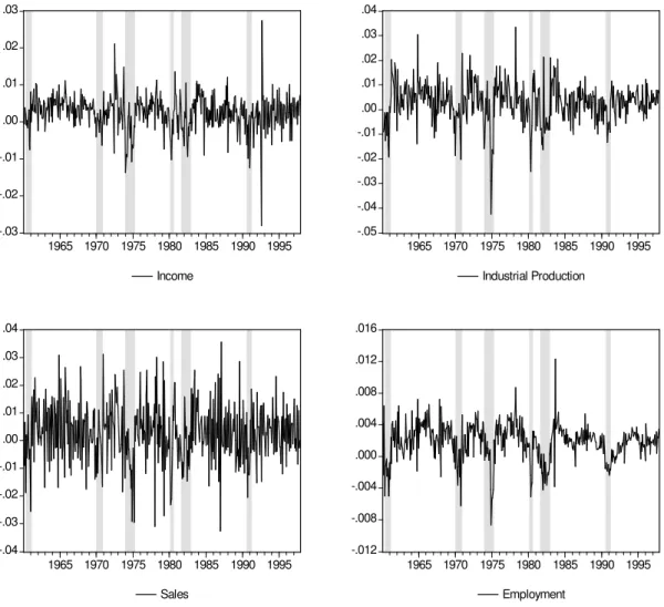
Our analysis is based on monthly data from 1960:01 to 1997:11. The four coincident series, “Income” (It), “Industrial Production” (Yt), “Employment” (Nt) and “Sales”
(St), are de…ned in Table 1 and their growth rates are plotted in Figure 1, where shaded
areas represent the NBER dating of recession periods. All four series show signs of dropping during recessions, although this behavior is more pronounced for Industrial Production (¢ lnYt) and Employment (¢ lnNt). These two series also show a more
visible cyclical pattern, whereas, for example, it is hard to notice the cyclical pattern in Sales(¢ lnSt) or Income(¢ lnIt). Before modelling the joint cyclical pattern of the
coincident series in(¢ lnIt; ¢ lnYt; ¢ lnNt; ¢ lnSt), we performed cointegration tests
to verify if the series in (lnIt;lnYt;lnNt;lnSt) share a common long-run component.
As in Stock and Watson (1989), we …nd no cointegration among these variables.
Conditional on the evidence of no cointegration for the elements of(lnIt;lnYt;lnNt;lnSt),
we model them as a Vector Autoregression (VAR) in …rst di¤erences. Besides
(¢ lnIt; ¢ lnYt; ¢ lnNt; ¢ lnSt) and their lags, the VAR also contains the lags of
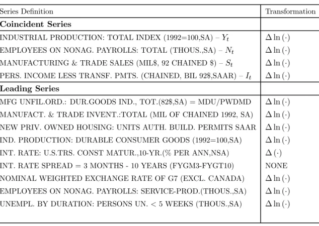
helpful in forecasting the coincident series. A list of these leading series is also presented in Table 1. They were used by Stock and Watson(1988a) and comprise a subset of the variables initially chosen by Burns and Mitchell (1946) to be leading indicators9.
The Akaike Information Criterion chose a VAR of order 2. However, the LM test on the residuals of a VAR(2) showed signs of signi…cant serial correlation in the errors. Since the canonical-correlation test is valid only if the model is dynamically well speci…ed10, we
increased the lag length until there were no signs of serial correlation left in the residuals of the system. This led to a VAR of order 4. Conditional on aV AR(4)we calculated the canonical correlations between the coincident series (¢ lnIt;¢ lnYt;¢ lnNt;¢ lnSt) and
the respective conditioning set, comprising four lags of (¢ lnIt;¢ lnYt;¢ lnNt;¢ lnSt)
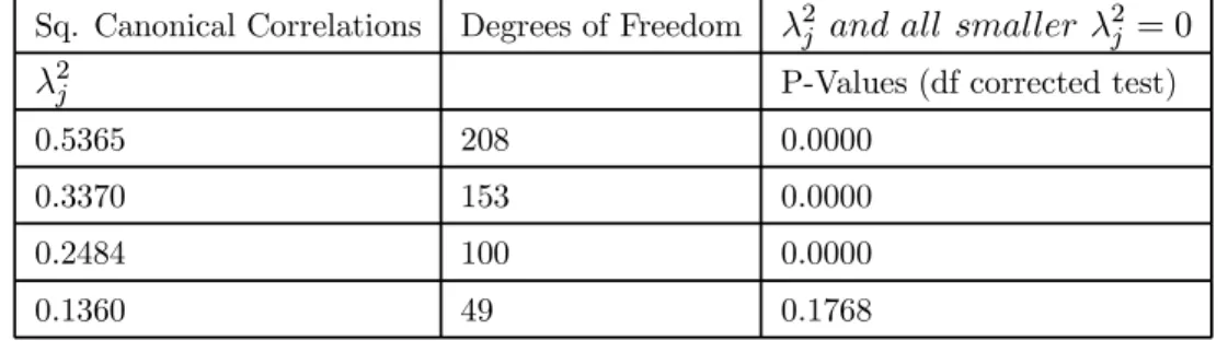
and four lags of the leading series. The canonical-correlation test results in Table 2 allow the conclusion that there is only one linear combination of the coincident series which is white noise. Hence, the cyclical behavior of (¢ lnIt; ¢ lnYt; ¢ lnNt; ¢ lnSt) can
be represented by three orthogonal canonical factors. These factors, (c1t; c2t; c3t), were
labelled as the coincident basis cycles and are a linear combination of the coincident series:
2 6 6 4
c1t
c2t
c3t
3 7 7 5= 2 6 6 4
0:45 ¡0:05 20:90 ¡0:52 1:43 ¡0:69 6:72 ¡4:78
¡0:87 ¡7:82 14:56 2:13
3 7 7 5£ 2 6 6 6 6 4
¢ lnIt
¢ lnYt
¢ lnNt
¢ lnSt
3 7 7 7 7 5 (7)
A correlation matrix of the three coincident and the three leading factors is presented in Table 3. To investigate their ability in explaining NBER recessions we include in this correlation matrix the NBER recession indicator dummy (which is equal to one during periods identi…ed by NBER as recessions and zero otherwise). As could be expected a priori, the …rst factor (either coincident or leading) is the one with the highest correlation
with the NBER dummy variable, followed by the second, and …nally by the third.
3.2
“The Missing Link”: using the NBER information in computing
the coincident index
The structural model in (4) enables us to incorporate the information in the NBER recession indicator in constructing a coincident index of economic activity. It also incor-porates the information resulting from the canonical correlation analysis, namely that there are only three signi…cant basis cycles in the four coincident series. We use the two stage conditional maximum likelihood (2SCML) estimator proposed by Rivers and Vuong (1988) to obtain instrumental variable estimates for the coe¢cients of each basis cycle.
9
Stock and Watson smooth some of these leading indicators. Here, we make no use of such transfor-mations.
10
The 2SCML estimates are presented in Table 4. After rewriting the basis cycles as linear combinations of the coincident series and normalizing the weights to add up to unity, we obtain our index (standard errors are given in parentheses):
¢IV CIt= 0:00
(0:01)£¢ lnIt+ 0(0::1006)£¢ lnYt+ 0(0::8406)£¢ lnNt+ 0(0::0602)£¢ lnSt: (8)
Equation (8) shows that most of the weight is given to employment, no weight is given to income, and that employment and industrial production together get 94% of the weight. A plot of this index is presented in Figure 2. This is not surprising given our previous analysis of Figure 1, since these two series have a more pronounced coherence with the NBER recession indicator. It also agrees with a memo of the Business Cycle Dating Committee (Hall et al. 2002, p. 9) where they state “employment is probably the single most reliable indicator [of recessions]”. It is interesting to compare our index with alternative indices in the literature. The corresponding weights that are used by the Conference Board to calculate the coincident index11are(0:28;0:13;0:48;0:11):The striking di¤erence between our weights and those of the TCB index is that income (It)
is weighed much more heavily in the TCB index than in ours, and employment(Nt) is
weighed more heavily in our index than in theirs.
In order to determine the sensitivity of the weights to the choice of three basis cycles, we have also computed our index using one, two and four basis cycles. When we use only one factor, the index is almost entirely based on the employment variable (weight of employment is almost 100%). As we increase the number of basis cycles, the weight of employment decreases to 0.91, 0.84 and 0.71 in the two, three and four factor models respectively. A four factor model is the one where all linear combinations of variables, even those which have no cyclical information, are included in the construction of the index. This shows that a large part of the di¤erence between our index and the other two indices is our decision to exclude the white noise linear combination of the series from the analysis.
Another aspect of sensitivity analysis concerns the stability of the structure over time. This includes the number of signi…cant basis cycles found and the coe¢cients of these basis cycles in the probit analysis. Starting from the …rst half of the sample and recursively estimating our model adding one observation at a time, we found almost invariably three signi…cant basis cycles at the 5% level of signi…cance. This reinforces our choice of three basis cycles in the construction of our index. The recursively estimated weights in equation (8) however show some variation over time. In particular, the weight of income has declined from 0.25 to 0.00, which is the only case where recursive estimates leave the 95% con…dence band of the initial estimates. This is consistent with the observation that income has not fallen substantially in recent recessions and hence
11
the NBER has reduced its weight in dating these recessions (see Hall et al, 2002). We leave the question of whether it would be useful to relax our assumption of a …xed weight coincident indicator for future research.
As a by-product of our analysis, we construct ¢IV LIt as in (3). We investigate
its predictive performance by running a probit regression where ¢IV LIt is used to
forecast the state of the economy. If we use a cutto¤ of 0.5, the model correctly predicts 97% of expansion periods and 62% of recession periods.Despite its good performance in identifying the state of the economy, it must be emphasized that ¢IV LIt is only a
one-step-ahead leading index, and that constructing multi-step-ahead leading indices are beyond the scope of this paper, since it involves dealing with non-linearity and causality.
3.3
Comparisons with Existing Coincident Indices
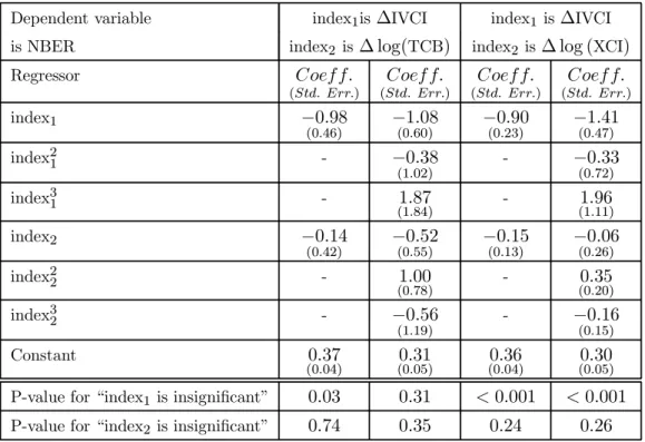
We perform the speci…cation tests described in Section 2.3 with regard to the TCB index and the experimental index12 (XCI) proposed by Stock and Watson (1989). The
results of estimating equations (5) and (6), once with the TCB index and once with the XCI index as the alternative index, are presented in Table 5. This table also shows the p-values of the null hypothesis of “given one index, the alternative index is insigni…cant” in each equation. It can be seen from this table that in a linear probability model, the coe¢cient of our index is signi…cant, whereas there is no evidence that the coe¢cients of the other two indices are signi…cantly di¤erent from zero. When we add the squares and cubes of indices to test equations, there is no evidence that, given our index, XCI and TCB indices have any additional explanatory power. However, when we perform the reverse test, we conclude that given XCI, our index has signi…cant explanatory power, but that given the TCB index it doesn’t. These tests indicate that, controlling for our index, there is no useful information in either the TCB or the XCI indices in explaining the business cycle state of the economy13.
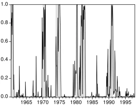
Our coincident index is designed to provide the best prediction of the state of the economy at timetgiven the information available at timet. Our probit analysis produces estimates of recession probabilities at each time period, conditional on the information available at that time14. Figure 3 plots these predicted probabilities. Based on a cuto¤ point of 0.5, the model predicts recessions and expansions with accuracy of 77% and 98% respectively. A naive comparison of the correct predictions of three probit regressions with IVCI, TCB and the XCI indices as explanatory variables shows that IVCI is more accurate in predicting recessions (46 correct predictions versus 37 for TCB and 31 for XCI), while all three indices perform equally well in predicting expansions. Note that
12We have downloaded this series from http://ksghome.harvard.edu/~.JStock.Academic.Ksg/xri/0012/xindex.asc. 13We also used the appropriately modi…ed “arti…cial regression” test of Davidson and McKinnon
(1993), and the results were qualitatively identical at the 5% signi…cance level.
this exercise uses only current information to predict the state of the economy.
This picture changes when we allow for “smoothing” using future information to detect turning points. We use the Bry and Boschan (1971) algorithm (a two-sided …lter) to extract peaks and troughs (i.e. turning points) of the three indices. We observe that, for turning points alone, the TCB index gets 9 out of the 12 turning points correctly, while IVCI gets 7 and XCI gets 6. For each index, time periods between peaks and troughs are labelled as recessions and assigned a value of one. Otherwise, periods are assigned a value of zero. These dummy variables are compared with the actual NBER Dating Committee’s dummy using a quadratic loss function. For the sample as a whole, TCB has a mean squared error of 0.9%, whereas IVCI and XCI have mean squared errors of 2.8% and 4.1% respectively. It is important to reiterate that our goal is to design an index that produces the best prediction of the state of economy based on the information available at timet;and not an index that produces the best prediction with the bene…t of hindsight. In real time, the user of the coincident index will not have future information to “smooth” the estimate of the likelihood of a recession. If the objective was to construct an index, whose Bry-Boschan smoothed states coincided with the NBER indicator, one could estimate the weights of coincident series that would produce the smallest mean squared error in that dimension. Our search over a two digit grid on the simplex resulted in 185 sets of weights that produced only two wrong predictions out of 450 data periods, which is half of the wrong predictions of the TCB index.15
4
Conclusion
The basic idea behind this paper is simple: use the information content in the NBER Business Cycle Dating Committee decisions to construct a coincident index of economic activity. Although several authors have devised sophisticated coincident indices with the ultimate goal of matching NBER recessions, no one has used the information in the NBER decisions to construct a coincident index. The second ingredient of our method is that we use canonical correlation analysis to …lter out the noisy information contained in the coincident series. As a result, our …nal index is only in‡uenced by the cyclical components of the coincident series. In our model, a structural equation relates the unobserved state of the economy to the cyclical components of the coincident series. We employ a two stage conditional maximum likelihood method to use the information in the NBER recession indicator about the unobserved state of the economy in order to estimate the parameters of this structural equation. The resulting index is a simple linear combination of the four coincident series originally proposed by Burns and Mitchell (1946).
15
As explained in the Introduction, we like to think that our method uncovers the “Missing Link” between the pioneering research of Burns and Mitchell (1946) and the deliberations of the NBER Business-Cycle Dating Committee. This is a consequence of the way we have constructed our coincident index: the coincident index is a linear combination of the four coincident series proposed by Burns and Mitchell that has a com-mon cycle with an unobserved state variable which is consistent with the deliberations of the NBER Business Cycle Dating Committee. It is noteworthy that our coincident index places the largest weight on employment (84%), which is in agreement with the opinion of the NBER Business Cycle Dating Committee (Hall et al., 2002, p. 9) that “employment is probably the single most reliable indicator [of recessions]”.
Our methodology also conveniently produces a one-step leading index of economic activity which is a linear combination of lags of coincident and leading variables. More-over, the probit model that produces our coincident index is, in fact, a model of the probability of recessions.
The performance of our constructed coincident index is promising. With speci…ca-tion tests against particular alternatives, we conclude that there is no gain in combining our index with either of the two currently popular coincident indices, namely the TCB and the XCI coincident indices. This means that, given our index, there is no useful information in the other two indices about the state of the economy. Although techni-cally we cannot conclude that our index encompasses the TCB and XCI indices, because those two indices do not use the information in the NBER dates in their construction, the speci…cation test results delineate the important question that motivated our pa-per, i.e., why do TCB and XCI indices ignore this vital piece of information in their construction?
In countries where there are no institutions similar to the NBER Business Cycle Dating Committee, simple rules such as two quarters of negative growth in the GDP or the quarterly version of the Bry and Boschan (1971) algorithm applied to quarterly GDP are used to identify recessions. A useful extension of the present paper will be to use our structural framework to identify the coincident index as the common cycle between the monthly coincident variables and the quarterly recession indicator or the quarterly GDP series. This extension is left for future research.
References
Akaike, H. (1976), “Canonical Correlation Analysis of Time Series and the Use of an Information Criterion”, in R.K. Mehra and D.G. Lainiotis (Eds) System Identi…-cation: Advances and Case Studies, New York: Academic Press, pp. 27-96.
Anderson, H. M. and F. Vahid (1998), “Testing Multiple Equation Systems for Com-mon Nonlinear Factors”, Journal of Econometrics,84, 1-37.
Balke, N.S. and T.B. Fomby (1997), “Threshold Cointegration”, International Eco-nomic Review, 38, 627-647.
Birchenhall, C., H. Jensen, D. Osborn and P. Simpson (1999), “Predicting US business cycle regimes”,Journal of Business and Economic Statistics, 17, 313-323.
Bry, G. and C. Boschan (1971),Cyclical Analysis of Time Series: Selected Procedures and Computer Programs, New York: NBER.
Burns, A. F. and Mitchell, W. C.(1946),Measuring Business Cycles. New York: Na-tional Bureau of Economic Research.
Chauvet, M. (1998), “An Econometric Characterization of Business Cycle Dynamics with Factor Structure and Regime Switching”, International Economic Review, 39, 969-996.
Davidson, R. and MacKinnon, J.G. (1993), “Estimation and Inference in Economet-rics,” Oxford: Oxford University Press.
Engle, R. F. and Kozicki, S. (1993), “Testing for Common Features”, Journal of Business and Economic Statistics, 11, 369-395, with discussions.
Engle, R. F. and Issler, J. V. (1995), “Estimating Sectoral Cycles Using Cointegration and Common Features”,Journal of Monetary Economics, 35, 83-113.
Estrella A. and F. S. Mishkin (1998), “Predicting U.S. Recessions: Financial Variables as Leading Indicators”, Review of Economics and Statistics, 80, 45-61.
Geweke, J. (1977), “The Dynamic Factor Analysis of Economic Time Series,” Chapter 19 in D.J. Aigner and A.S. Goldberger (eds) Latent Variables in Socio-Economic Models, Amsterdam: North Holland.
Hall, R., Feldstein, M., Bernanke, B., Frankel, J., Gordon, R. and Zarnowitz, V. (2002), “The NBER’s Business-Cycle Dating Procedure”, downloadable from http://www.nber.org/cycles/november2001/recessions.pdf.
Hamilton, J.D. (1994),Time Series Analysis, Princeton: Princeton University Press.
Hamilton, J.D. (1989), “A New Approach to the Economic Analysis of Nonstationary Time Series and the Business Cycle”,Econometrica, 57, 357-384.
Hecq, A., F. Palm and J.P. Urbain (2000), “Permanent-Transitory Decomposition in VAR Models with Cointegration and Common Cycles”, Oxford Bulletin of Eco-nomics and Statistics, 62, 511-532.
Hotelling, H. (1935), “The Most Predictable Criterion”,Journal of Educational Psy-chology, 26, 139-142.
Hotelling, H. (1936), “Relations Between Two Sets of Variates”,Biometrika, 28, 321-377.
Issler, J.V. and Vahid, F. (2001), “Common Cycles and the Importance of Transitory Shocks to Macroeconomic Aggregates,”Journal of Monetary Economics, 47, 449-475.
Lahiri, K. and G. Moore (1993), Editors, “Leading Economic Indicators: New Ap-proaches and Forecasting Records.” New York: Cambridge University Press.
Mizon, G.E. (1984), “The Encompassing Approach in Econometrics”, Chapter 6 in D.F. Hendry and K.F. Wallis (eds) Econometrics and Quantitative Economics, Oxford: Blackwell.
Newey, W. and K. West (1987), “A Simple Positive Semi-De…nite, Heteroskedasticity and Autocorrelation Consistent Covariance Matrix,” Econometrica, 55, 703-708.
Rivers, D. and Q.H. Vuong (1988), “Limited Information Estimators and Exogeneity Tests for Simultaneous Probit Models”,Journal of Econometrics, 39, 347-366.
Stock, J. and Watson, M.(1988a), “A New Approach to Leading Economic Indicators,” mimeo, Harvard University, Kennedy School of Government.
Stock, J. and Watson, M.(1988b), “A Probability Model of the Coincident Economic Indicator”, NBER Working Paper # 2772.
Stock, J. and Watson, M.(1989) “New Indexes of Leading and Coincident Economic Indicators”, NBER Macroeconomics Annual, pp. 351-95.
Stock, J. and Watson, M.(1991), “A Probability Model of the Coincident Economic Indicators”, in “Leading Economic Indicators: New Approaches and Forecasting Records,” K. Lahiri and G. Moore, Eds. New York: Cambridge University Press.
Stock, J. and Watson, M.(1993a), “A Procedure for Predicting Recessions with Lead-ing Indicators: Econometric Issues and Recent Experiences,” in “New Research on Business Cycles, Indicators and Forecasting,” J.H. Stock and M.W. Watson,
Stock, J. and Watson, M.(1993b), Editors, “New Research on Business Cycles, Indi-cators and Forecasting” Chicago: University of Chicago Press, for NBER.
The Conference Board (1997), “Business Cycle Indicators,” Mimeo, The Conference Board, downloadable from http://www.tcb-indicators.org/bcioverview/bci4.pdf.
Vahid, F. and Engle, R. F. (1993), “Common Trends and Common Cycles”,Journal of Applied Econometrics, 8, 341-360.
Vahid, F. and Engle, R.F.(1997), “Codependent Cycles,”Journal Econometrics, vol. 80, pp. 199-121.
Watson, M.W. (1994), “Business-Cycle Durations and Postwar Stabilization of the U.S. Economy,” American Economic Review, 84, 24-46.
Wooldridge, J.M.(1994), “Estimation and Inference for Dependent Processes,” in “Handbook of Econometrics IV,” R.F. Engle and D. McFadden, Editors. Ams-terdam: Elsevier Press.
Zellner, A. and C. Min (1999), “Forecasting Turning Points in Countries’ Output Growth Rates”,Journal of Econometrics, 88, 203 - 206.
A
Appendices
A.1
Statistical foundation of TCB and XCI indices
A coincident index, which is widely used by practitioners, is the index constructed by The Conference Board – TCB. This coincident index is a weighted average of the coincident variables – employment, output, sales and income, where weights are the reciprocal of the standard deviation of each component’s growth rate and add up to unity; see The Conference Board (1997).
Stock and Watson’s experimental coincident index(XCI)is based on an “unobserved single index” or “dynamic factor” model; see Geweke(1977), for example. There, the growth rate of the four coincident series (output, sales, income and employment) share
a common cycle,¢XCIt, which is a latent dynamic factor that represents (the change
in) “the state of the economy.” Denoting the growth rates of the coincident series as the vectorxt= (x1t; x2t; x3t; x4t)
0
;their proposed statistical model is as follows:
xt = ¯+°(L)¢XCIt+ut;
Á(L)¢XCIt = ±+´t;
whereÁ(L)and°(L)are scalar polynomials on the lag operatorL, andD(L)is a matrix
polynomial onL. The error structure is restricted so as to haveE 2 4 Ã ´t ²t ! Ã ´t ²t
!03
5=
diag(¾2´; ¾2² 1; :::; ¾
2
²4), andD(L) =diag[dii(L)], which makes innovations mutually
uncor-related.
The model (9) assumes that there is a single source of comovement among the growth rates of the coincident series –¢XCIt. Still, these series are allowed to have their own
idiosyncratic cycle, since the vector of error terms ut is composed of serially correlated
components that are mutually orthogonal. Hence, each of the four coincident series in
xt has two cyclical components: a common and an idiosyncratic one. In this view, the
“business cycle” is the intersection of the cycles in output, income, employment, and trade. Moreover, there is no guarantee that idiosyncratic cycles do not dominate the common cycle in explaining the variation of the four series in xt:
In contrast, in our view the “business cycle” is the union of the cycles in output, income, employment, and trade. There are no idiosyncratic cycles that can be put aside, the only part ofxtthat we leave out is the non-cyclical combination resulting from the
canonical correlation analysis. Comparing our method with Stock and Watson’s clearly shows that neither model is a special case of the other. Hence, neither model is nested within the other one, and comparisons between them have to be made using non-nested tests. Chauvet (1998) has generalized the framework in Stock and Watson by allowing a two-state mean for the latent factor ¢XCIt in (9), representing recession and
non-recession regimes.
A.2
Two stage conditional maximum likelihood estimation
Denoting by c1t;¢ ¢ ¢ ; ckt; (cit =®0ixt; i= 1;¢ ¢ ¢; k); the k basis cycles associated with
the …rst knon-zero canonical correlations, the NBER business-cycle indicator is linked to them through the latent variabley¤
t:
E(y¤t j It+h) =¯0+¯1c1t+¢ ¢ ¢+¯kckt+ut (10)
NBERt =
(
1 ifE(y¤
t jIt+h)<0
0 otherwise. :
The possible correlation betweenc1t;¢ ¢ ¢; ckt and the errors ut is modelled as follows,
cit = ¸i
¡ °0izt
¢
+vit; i= 1;¢ ¢ ¢ ; k (11)
à ut vt ! » N à 0; "
¾2u ¾0
vu
¾vu §vv
#!
where the vit,i= 1;¢ ¢ ¢; k, are collected into a k-vector vt,¸i and °0izt fori= 1;¢ ¢ ¢ ; k
come from the canonical-correlation analysis,§vvis ak£kdiagonal variance-covariance
measurement error, the basis cycles c1t;¢ ¢ ¢; ckt are correlated withut. Joint normality
of ut and vt implies:
ut=vt0±+´t
where±= §¡1
vv¾vu; ´t»N
¡
0; ¾2u¡¾0
vu§
¡1
vv¾vu¢and´tis independent ofvt:Substituting
forutin equation (10), we obtain,
E(yt¤ j It+h) =¯0+¯1c1t+¢ ¢ ¢+¯kckt+v
0
t±+´t (12)
NBERt =
(
1 if´t<¡(¯0+¯1c1t+¢ ¢ ¢+¯kckt+v0t±)
0 if´t¸ ¡(¯0+¯1c1t+¢ ¢ ¢+¯kckt+v0t±)
:
Notice that, by construction, all the regressors in (12) are uncorrelated with the error term ´t. As usual for probit models, the mean parameters µ= ¡¯0; ¯1; ¯2; ¯3; ±0¢0
and the variance parameter ¡¾2´ =¾2u¡¾0
vu§
¡1
vv¾vu
¢
are not separately identi…able. The convenient normalization ¾2´ = 1 will identify the mean parameters. Obtaining the two stage conditional maximum likelihood (2SCML) estimator proposed by Rivers and Vuong (1988) entails the following steps:
1. Regress cit,i= 1;¢ ¢ ¢ ; k, on ztto get bvit and§bvv, a consistent estimate of§vv.
2. From bvit, i= 1;¢ ¢ ¢ ; k, form bvt and then run a probit regression (12) to get
con-sistent estimates ofµ=¡¯0; ¯1; ¯2; ¯3; ±0¢0, denoted by bµ.
For inference onµ, if´t is i.i.d., the following central-limit theorem holds:
p
T³bµ¡µ´¡!d N(0; V);
where the appropriate formula for the asymptotic covariance matrixV is given in Rivers and Vuong (1988, p. 354).
The error term´tin (12), as explained in the text, is likely to be a moving average process since the NBER dating committee uses future information in deciding on the state of the economy. Since this future information is unpredictable at time t;it is still valid to useztas instruments for estimation. However, autocorrelation robust standard
B
Tables and …gures
Table 1: Coincident and Leading Series: De…nitions and Transformations
Series De…nition Transformation
Coincident Series
INDUSTRIAL PRODUCTION: TOTAL INDEX (1992=100,SA) –Yt ¢ ln (¢)
EMPLOYEES ON NONAG. PAYROLLS: TOTAL (THOUS.,SA) –Nt ¢ ln (¢)
MANUFACTURING & TRADE SALES (MIL$, 92 CHAINED $) –St ¢ ln (¢)
PERS. INCOME LESS TRANSF. PMTS. (CHAINED, BIL 92$,SAAR) –It ¢ ln (¢)
Leading Series
Table 2: Squared Canonical Correlations and Canonical-Correlation Test
Sq. Canonical Correlations Degrees of Freedom ¸2j and all smaller ¸2j = 0
¸2j P-Values (df corrected test)
0.5365 208 0.0000
0.3370 153 0.0000
0.2484 100 0.0000
0.1360 49 0.1768
Table 3: Correlation Matrix for Factors and NBER Recession-Indicator
Basis Basis Basis Leading Leading Leading NBER Cycle 1 Cycle 2 Cycle3 Factor 1 Factor 2 Factor 3
NBER 1
Basis Cycle 1 0.60 1
Basis Cycle 2 0.15 0 1
Basis Cycle 3 0.15 0 0 1
Leading Factor 1 0.63 0.73 0 0 1
Leading Factor 2 0.14 0 0.58 0 0 1
Table 4: Two Stage Conditional Maximum Likelihood Estimates
Regressor Est. Coe¤. Std. Error
c1t 65.21 8.86
c2t 28.05 6.41
c3t 13.00 6.75
Constant -0.33 0.19
p-value of overall signi…cance <0.01
McFadden R-Squared 0.71
% overall correct prediction 94.89
Table 5: Speci…cation Test Results
Dependent variable index1is¢IVCI index1 is¢IVCI is NBER index2 is¢ log(TCB) index2 is¢ log (XCI)
Regressor Coef f:
(Std: Err:)
Coef f:
(Std: Err:)
Coef f:
(Std: Err:)
Coef f:
(Std: Err:)
index1 ¡0:98
(0:46) ¡1
:08
(0:60) ¡0
:90
(0:23) ¡1
:41
(0:47)
index21 - ¡0:38
(1:02)
- ¡0:33
(0:72)
index31 - 1:87
(1:84) - (11::9611)
index2 ¡0:14
(0:42) ¡0
:52
(0:55) ¡0
:15
(0:13) ¡0
:06
(0:26)
index22 - 1:00
(0:78) - (00::3520)
index32 - ¡0:56
(1:19) - ¡0
:16
(0:15)
Constant 0:37
(0:04) (00::3105) (00::3604) (00::3005) P-value for “index1 is insigni…cant” 0:03 0:31 <0:001 <0:001 P-value for “index2 is insigni…cant” 0:74 0:35 0:24 0:26
In both tables, all equations are estimated using 4 lags of coincident and leading variables as instruments. The standard errors and p-values are calculated using the Newey-West estimator of the
-.03 -.02 -.01 .00 .01 .02 .03
1965 1970 1975 1980 1985 1990 1995
Income
-.05 -.04 -.03 -.02 -.01 .00 .01 .02 .03 .04
1965 1970 1975 1980 1985 1990 1995
Industrial Production
-.04 -.03 -.02 -.01 .00 .01 .02 .03 .04
1965 1970 1975 1980 1985 1990 1995
Sales
-.012 -.008 -.004 .000 .004 .008 .012 .016
1965 1970 1975 1980 1985 1990 1995
Employment
- . 0 3 - . 0 2 - . 0 1 . 0 0 . 0 1 . 0 2 . 0 3
6 5 7 0 7 5 8 0 8 5 9 0 9 5
X C I
- . 0 3 - . 0 2 - . 0 1 . 0 0 . 0 1 . 0 2 . 0 3
6 5 7 0 7 5 8 0 8 5 9 0 9 5
T C B
- . 0 3 - . 0 2 - . 0 1 . 0 0 . 0 1 . 0 2 . 0 3
6 5 7 0 7 5 8 0 8 5 9 0 9 5
I V C I
0.0 0.2 0.4 0.6 0.8 1.0
1965 1970 1975 1980 1985 1990 1995