❊♥s❛✐♦s ❊❝♦♥ô♠✐❝♦s
❊s❝♦❧❛ ❞❡
Pós✲●r❛❞✉❛çã♦
❡♠ ❊❝♦♥♦♠✐❛
❞❛ ❋✉♥❞❛çã♦
●❡t✉❧✐♦ ❱❛r❣❛s
◆◦ ✹✹✺ ■❙❙◆ ✵✶✵✹✲✽✾✶✵
❚❤❡ ▼✐ss✐♥❣ ▲✐♥❦✿ ❯s✐♥❣ t❤❡ ◆❇❊❘ ❘❡❝❡s✲
s✐♦♥ ■♥❞✐❝❛t♦r t♦ ❈♦♥str✉❝t ❈♦✐♥❝✐❞❡♥t ❛♥❞
▲❡❛❞✐♥❣ ■♥❞✐❝❡s ♦❢ ❊❝♦♥♦♠✐❝ ❆❝t✐✈✐t②
❏♦ã♦ ❱✐❝t♦r ■ss❧❡r✱ ❋❛rs❤✐❞ ❱❛❤✐❞
❖s ❛rt✐❣♦s ♣✉❜❧✐❝❛❞♦s sã♦ ❞❡ ✐♥t❡✐r❛ r❡s♣♦♥s❛❜✐❧✐❞❛❞❡ ❞❡ s❡✉s ❛✉t♦r❡s✳ ❆s
♦♣✐♥✐õ❡s ♥❡❧❡s ❡♠✐t✐❞❛s ♥ã♦ ❡①♣r✐♠❡♠✱ ♥❡❝❡ss❛r✐❛♠❡♥t❡✱ ♦ ♣♦♥t♦ ❞❡ ✈✐st❛ ❞❛
❋✉♥❞❛çã♦ ●❡t✉❧✐♦ ❱❛r❣❛s✳
❊❙❈❖▲❆ ❉❊ PÓ❙✲●❘❆❉❯❆➬➹❖ ❊▼ ❊❈❖◆❖▼■❆ ❉✐r❡t♦r ●❡r❛❧✿ ❘❡♥❛t♦ ❋r❛❣❡❧❧✐ ❈❛r❞♦s♦
❉✐r❡t♦r ❞❡ ❊♥s✐♥♦✿ ▲✉✐s ❍❡♥r✐q✉❡ ❇❡rt♦❧✐♥♦ ❇r❛✐❞♦ ❉✐r❡t♦r ❞❡ P❡sq✉✐s❛✿ ❏♦ã♦ ❱✐❝t♦r ■ss❧❡r
❉✐r❡t♦r ❞❡ P✉❜❧✐❝❛çõ❡s ❈✐❡♥tí✜❝❛s✿ ❘✐❝❛r❞♦ ❞❡ ❖❧✐✈❡✐r❛ ❈❛✈❛❧❝❛♥t✐
❱✐❝t♦r ■ss❧❡r✱ ❏♦ã♦
❚❤❡ ▼✐ss✐♥❣ ▲✐♥❦✿ ❯s✐♥❣ t❤❡ ◆❇❊❘ ❘❡❝❡ss✐♦♥ ■♥❞✐❝❛t♦r t♦ ❈♦♥str✉❝t ❈♦✐♥❝✐❞❡♥t ❛♥❞ ▲❡❛❞✐♥❣ ■♥❞✐❝❡s ♦❢ ❊❝♦♥♦♠✐❝ ❆❝t✐✈✐t②✴ ❏♦ã♦ ❱✐❝t♦r ■ss❧❡r✱ ❋❛rs❤✐❞ ❱❛❤✐❞ ✕ ❘✐♦ ❞❡ ❏❛♥❡✐r♦ ✿ ❋●❱✱❊P●❊✱ ✷✵✶✵
✭❊♥s❛✐♦s ❊❝♦♥ô♠✐❝♦s❀ ✹✹✺✮
■♥❝❧✉✐ ❜✐❜❧✐♦❣r❛❢✐❛✳
The Missing Link: Using the NBER Recession Indicator
to Construct Coincident and Leading Indices of Economic
Activity
1João Victor Issler2
Graduate School of Economics — EPGE Getulio Vargas Foundation Praia de Botafogo 190 s. 1100
Rio de Janeiro, RJ 22253-900 Brazil
Farshid Vahid
Department of Econometrics and Business Statistics Monash University
P.O. Box 11E Victoria 3800
Australia
This Version: May, 2002
1Acknowledgments: João Victor Issler acknowledges the hospitality of Monash University and Farshid Vahid acknowledges the hospitality of the Getulio Vargas Foundation. We have ben-eÞted from comments and suggestions of Heather Anderson, Antonio Fiorencio, Clive Granger, Don Harding, Alain Hecq, Soren Johansen, Carlos Martins-Filho, Helio Migon, Ajax Moreira, Adrian Pagan, and Mark Watson, who are not responsible for any remaining errors in this paper. João Victor Issler acknowledges the support of CNPq-Brazil and PRONEX. Farshid Vahid is grateful to the Australian Research Council Small Grant scheme and CNPq Brazil for Þnancial assistance.
Abstract
We use the information content in the decisions of the NBER Business Cycle Dat-ing Committee to construct coincident and leadDat-ing indices of economic activity for the United States. We identify the coincident index by assuming that the coincident vari-ables have a common cycle with the unobserved state of the economy, and that the NBER business cycle dates signify the turning points in the unobserved state. This model allows us to estimate our coincident index as a linear combination of the coinci-dent series. We establish that our index performs better than other currently popular coincident indices of economic activity.
Keywords: Coincident and Leading Indicators, Business Cycle, Canonical Correlation,
Instrumental Variable Probit, Encompassing.
1
Introduction
Suppose that we are asked to construct an index of health status of a patient. Also, suppose that we know that the best indicator of the health of the patient is the results of a blood test. However, blood samples cannot be taken too frequently, and test results are only available with a lag, sometimes too long to be useful. Our index therefore must be a function of variables such as blood pressure, pulse rate and body temperature that are readily available at regular frequencies. In order to estimate the best way to combine these variables into an index, would we (i) use the historical data on these variables only, or, (ii) use the historical blood test results as well? The answer is, obviously, the latter. This analogy, we hope, illustrates what is missing in the recent attempts to construct new coincident indices of economic activity for the United States. In this literature, researchers have used historical data on coincident series only, and ignored the vital information in the NBER recession indicator.
Since Burns and Mitchell (1946) there has been a great deal of interest in making inference about the “state of the economy” from sets of monthly variables that are believed to be either concurrent or to lead the economy’s business cycles (the so called “coincident” and “leading” indicators respectively). Although the business-cycle status of the economy is not directly observable, our most educated estimate of its turning points is embodied in the binary variable announced by the NBER Business Cycle Dating Committee. These announcements are based on the consensus of a panel of experts, and they are made some time (usually six months to one year) after the time of a turning point in the business cycle. NBER summarizes its deliberations as follows:
“The NBER does not deÞne a recession in terms of two consecutive quarters
of decline in real GNP. Rather, a recession is a recurring period of decline in total output, income, employment, and trade, usually lasting from six months to a year, and marked by widespread contractions in many sectors of the economy.”
(Quoted from http://www.nber.org/cycles.html)
indices have been proposed that are based on sophisticated statistical methods of ex-tracting a common latent dynamic factor from the coincident variables that comprise the traditional index; see, e.g., Stock and Watson (1988a, 1988b, 1989, 1991, 1993a), and Chauvet (1998).
The basic idea behind this paper is simple: use the information content in the NBER Business Cycle Dating Committee decisions, which are generally accepted as the chronology of the U.S. business-cycles1, to construct a coincident and a leading index of economic activity.
The NBER’s Dating Committee decisions have been used extensively to validate various models of economic activity. For example, to support his econometric model, Hamilton (1989) compares the smoothed probabilities of the “recessionary regime” im-plied by his Markov switching model with the NBER recession indicator. Since then, this has become a routine exercise for evaluating variants of Markov-switching models, see Chauvet (1998) for a recent example. Stock and Watson (1993a) use the NBER re-cession indicator to develop a procedure to validate the predictive performance of their experimental recession index. Estrella and Mishkin (1998) use the NBER recession indi-cator to compare the predictive performance of potential leading indiindi-cators of economic activity. However, as far as we know, no one has actually used the NBER recession
indi-cator toconstruct coincident and leading indicators. We therefore ask “Why not?”. In
our opinion, this is much more appealing than imposing stringent statistical restrictions to construct a common latent dynamic factor, hoping that it represents the economy’s business cycle.
The method that we employ here is based on a structural equation that links the NBER recession indicator to the coincident series. Because we are interested in con-structing indices of business-cycle activity, we only use the cyclical parts of the coincident series in this structural equation. This ensures that noise in the coincident series does not affect the Þnal index2. We estimate this equation using limited information quasi-maximum likelihood method. Natural candidates for the instrumental variables used in this method are the variables that are traditionally used to construct the leading index.
With formal speciÞcation tests we establish that data does not reject the assumptions
of our model.
The coincident index proposed here is a simple Þxed-weight linear combination of
the coincident series. Likewise, our leading index is also a simple Þxed-weight linear
combination of the leading series. This means that coincident and leading indices will be readily available to all users, who will not have to wait for them to be calculated and announced by a third party. The indices constructed by The Conference Board — TCB,
1See Stock and Watson (1993a, p. 98).
2The extraction of the cyclical part of the coincident series is performed using canonical-correlation
formerly constructed by the Department of Commerce, are used much more widely than other proposed indices, because of their ready availability.
We like to think that our method uncovers the “Missing Link” between the pioneer-ing research of Burns and Mitchell (1946), who proposed the coincident and leadpioneer-ing variables to be tracked over time, and the deliberations of the NBER Business Cycle
Dating Committee who deÞne a recession in terms of these same coincident variables
as “... a recurring period of decline in total output, income, employment, and trade, usually lasting from six months to a year, and marked by widespread contractions in many sectors of the economy”. Another feature of the present research effort is that it
integrates two different strands of the modern macroeconometrics literature. The Þrst
seeks to construct indices of and to forecast business-cycle activity, and is perhaps best
exempliÞed by the work of Stock and Watson (1988a, 1988b, 1989, 1991, 1993a), the
collection of papers in Lahiri and Moore (1993) and in Stock and Watson (1993b). The second seeks to characterize and test for common-cyclical features in macroeconomic data, where abusiness-cycle feature is regarded as a similar pattern of serial-correlation
for different macroeconomic series, showing that they display short-run co-movement;
see Engle and Kozicki (1993), Vahid and Engle (1993, 1997), and Hecq, Palm and Ur-bain (2000) for the basic theory and Engle and Issler (1995) and Issler and Vahid (2001) for applications.
The structure of the rest of the paper is as follows. In Section 2 we present the basic ingredients of our methodology in a non-technical way, leaving the technical details for the Appendix. Section 3 presents the coincident and leading indices, and Section 4 concludes.
2
Theoretical underpinning of the indexes
In this Section we explain the method that we use for constructing the coincident and leading indices of economic activity. Technical details are included in the Appendix.
2.1 Determining a basis for the cyclical components of coincident vari-ables
We require that the coincident index be a linear combination of the cyclical components of coincident variables. This means that in our view, the “business cycle” is a linear
combination of the cycles of the four coincident series (output, income, employment
and trade), and there is no unimportant cyclical ßuctuation in these variables that is
excluded. This contrasts with the single latent dynamic index view of a coincident index (e.g., Stock and Watson 1989 and Chauvet 1998), which restricts the “business cycle” to be a single common cyclical factor shared by the coincident variables. In order to
coincident variables to have other idiosyncratic cyclical factors, and this provides no control over how strong these idiosyncratic cycles are relative to the common cycle; see the discussion in Appendix A.1.
We deÞne as “cyclical” any variable which can be linearly predicted from the past
information set3. The past information set includes lags of both sets of coincident
and leading variables. The inclusion of lags of leading variables in addition to lags of coincident variables in the information set, in effect, serves two purposes. First, it combines the estimation of coincident and leading indicator indices. Second, it allows for the possibility of asymmetric cycles in coincident series by including lags of variables such as interest rates and the spread between interest rates which are known to be nonlinear processes (Anderson 1997, Balke and Fomby 1997) as exogenous predictors. There are inÞnitely many linear combinations of the coincident variables that are predictable from the past, that is, that are cyclical. We use canonical-correlation analysis toÞnd a basis for the space of these cycles.
Canonical-correlation analysis, introduced by Hotelling (1935, 1936), has been used
in multivariate statistics for a long time. It was Þrst used in multivariate time
se-ries analysis by Akaike (1976). Akaike aptly referred to the canonical variates as “the channels of information interface between the past and the present” and he referred to canonical correlations as the “strength” of these channels. We explain the concept brießy in our context, leaving more technical details for the Appendix.
Denote the set of coincident variables (income, output, employment and trade) by the vectorxt= (x1t, x2t, x3t, x4t)
0
and the set ofm(m≥4)“predictors” by the vectorzt(this includes lags ofxtas well as lags of the leading variables). Canonical correlations analysis transformsxtinto four independent linear combinationsA(xt) = (α01xt,α02xt,α03xt,α04xt)
with the property that α0
1xt is the linear combination of xt that is most (linearly) predictable from zt, α02xt is the second most predictable linear combination of xt from ztafter controlling forα01xt,and so on4. These linear combinations will be uncorrelated with each other and they are restricted to have unit variances so as to identify them uniquely up-to a sign change. By-products of this analysis are four linear combination of
3Although this de
Þnition may sound different from the engineering deÞnition of “cyclical”, which is
a process that is explained by dominant regular periodic functions (such as cosine waves), it is similar to it. Cramér Representation Theorem states that any stationary process can be written as integrals of cosine and sine functions of different frequencies with independent stochastic amplitudes, and as long as the process is not white noise, some of these periodic functions will dominate the rest in explaining
the total variation in the process. This justiÞes using “not white noise” or “predictable from the past”
as a deÞnition for “cyclical”.
4The fact that canonical correlations analysis studies channels oflinear dependence betweenxand
z does not necessarily imply that it will be only useful for linear multivariate analysis. By including
nonlinear basis functions (e.g. Fourier series, Tchebyschev polynomials) in z, one can use canonical
zt,Γ(zt) = (γ10zt,γ02zt,γ03zt,γ04zt),with the property thatγ0izt is the linear combination of zt that has the highest squared correlation with α0ixt, for i = 1,2,3,4. Again, the elements of Γ(zt) are uncorrelated with each other, and they are uniquely identiÞed up-to a sign switch with the additional restriction that all four have unit variances. The regressionR2betweenα0
ixtandγ0iztfori=1,2,3,4,which we denote by ¡
λ21,λ22,λ23,λ24¢, are the squared canonical correlations between xt and zt.
In the present application, we call (α0
1xt,α02xt,α03xt,α04xt) the “basis cycles” in xt. Our view that cycles are predictable from the past information, justiÞes using this term. It is important to note that moving fromxttoA(xt)is just a change of coordinates. In particular, no structure is placed on these variables from outside, and no information is thrown away in this transformation. Hence, the information content in A(xt)is neither more nor less than the information content in xt.
The advantage of this basis change is that it allows us to determine if the cyclical be-havior of the coincident series can be explained by less than four basis cycles. Note that in the Þrst basis cycle, i.e. the linear combination of xt with maximal correlation with the past, reveals the combination of coincident series with the most pronounced cycli-cal feature. Analogously, the linear combination associated with the minimal canonicycli-cal correlation reveals the combination of the xt with the weakest cyclical feature. We can use a simple statistical-test procedure to examine whether the smallest canonical corre-lation (or a group of canonical correcorre-lations) is statistically equal to zero; see Appendix A.2. If this hypothesis is not rejected, then the linear combination corresponding to the statistically insigniÞcant canonical correlation cannot be predicted from the past, i.e. it is white-noise, and therefore can be dropped from the set of basis cycles. In that case, we can conclude that all cyclical behavior in the four coincident series can be written in terms of less than four basis cycles.
Hence, the use of linear combination of xt’s that are not associated with a zero
canonical correlation is equivalent to using only the cyclical components of the coincident series. Any linear combination of the signiÞcant basis cycles is a linear combination of coincident variables, which is convenient for our purposes, because it implies that our coincident index will be a linear combination of the coincident variables themselves.
2.2 Estimating a structural equation for the unobserved business cycle state
One might think that to estimate the weights associated with each basis cycle it suffices to estimate a simple probit model with the NBER indicator as the binary dependent variable and the basis cycles associated with the non-zero canonical correlations as ex-planatory variables. Since the basis cycles are linear combinations of the four coincident series, we will ultimately end up explaining the NBER indicator by a linear combina-tion of the coincident series. However, it is important to note that the coincident index that we are after is a linear combination of the coincident series that has cyclical fea-tures similar to the unobserved state of the economy5. The NBER recession indicator is
important because it embodies some information about the unobserved business cycle state of the economy. As it will be clear below, the linear combination of the coincident series that has a serial correlation pattern similar to that of the unobserved state of the economy, is neither the conditional expectation of the NBER recession indicator given the past information set, nor the conditional expectation of the NBER indicator given the coincident series.
We state the key assumption that enables us to estimate the coincident index here:
Assumption 1: There exists a linear index of (the cyclical parts of) the coincident
series that has the exact same correlation pattern with the past information as the unobserved state of the economy.
Note that we have enclosed “the cyclical parts of” in parentheses because it is redun-dant. Although the index that has the same correlation pattern with the past will only involve the signiÞcant basis cycles (i.e. will not involve white noise combinations of the coincident series), these basis cycles are themselves linear combinations of coincident series. Hence, the index will ultimately be a linear combination of coincident series.
Let y∗
t denote the unobserved state of the economy and {c1t, c2t, c3t} denote the signiÞcant basis cycles of the coincident series at time t. Assumption 1 clearly implies
that there must be a linear combination of y∗
t and {c1t, c2t, c3t} that is unpredictable from the information before time t. That is,
E(y∗
t −β0−β1c1t−β2c2t−β3c3t|It−1) = 0. (1) whereIt−1is the information available at timet−1.Ifyt∗was observed, we could estimate
β1,β2 and β3 directly by GMM or limited information maximum likelihood.
However,y∗
t is not observed. Instead, we have the NBER indicator that is equal to 1
when, to the best knowledge of the NBER Dating Committee at timet+h,the economy
5Using the technical terms introduced in Engle and Kozicki (1993), we are assuming that the
unob-served business cycle state of the economy and the coincident variables have aserial correlation common
was in a recession at time t. That is, when the “smoothed” estimate of the unobserved state of the economy based on information at time t+his below a critical value6.
NBERt= (
1 ifE(y∗
t |It+h)<0
0 otherwise.
Using equation (1), we obtain:
E(y∗
t |It−1) = β0+β1E(c1t|It−1) +β2E(c2t|It−1) +β3E(c3t|It−1) = β0+β1c1t+β2c2t+β3c3t+ωt, whereE(ωt|It−1) = 0,
and obviouslyωt is correlated withcit, i=1,2,3.Because we can always write
E(yt∗|It+h) =E(y∗t |It−1) +ξt+ξt+1· · ·+ξt+h,
whereξt+i is the “surprise” associated with new information arriving in period t+i. It is straightforward to show that:
E(y∗t |It+h) = β0+β1c1t+β2c2t+β3c3t+ut, ut = ωt+ξt+ξt+1· · ·+ξt+h,
where ut is unforecastable given information at time t−1, i.e., E(ut|It−1) = 0, has a “forward” M A(h) structure, and is correlated with cit, i=1,2,3.
In order to estimateβ1,β2 andβ3 consistently, we need to use an estimation method designed for estimation of a single structural equation with a limited dependent vari-able. All of such methods use instrumental variables. In our case, obvious instrumental variables would be the zt variables (i.e. lags of coincident and leading variables). No-tice that canonical-correlation analysis produces estimates of γ0
1zt,γ02zt,γ03zt,andγ04zt, which are the best linear predictors for each of the basis cycles respectively.
Several alternative estimators have been proposed for the consistent estimation of parameters of a single equation with a limited dependent variable in a simultaneous equations model. These estimators differ in their ease of calculation versus their degree
of efficiency. We use the two stage conditional maximum likelihood (2SCML) estimator
proposed by Rivers and Vuong (1988) due to its relative simplicity. Because we ignore
the dynamic structure of ut in constructing the likelihood function, i.e., the model
is “dynamically incomplete” in the sense of Wooldridge (1994), autocorrelation-robust standard errors have to be used; see the Appendix for details.
Using the empirical results that will be presented fully in the next section, we as-sume that the four coincident series can be explained by three signiÞcant basis cycles
6
{c1t, c2t, c3t}. Denoting the NBER indicator byNBERt,theÞrst stage of the 2SCML es-timation involves regressing{c1t, c2t, c3t}on the instrumentsztand saving the residuals, which we denote by{ˆv1t,vˆ2t,vˆ3t}.In the second stage, both the basis cycles{c1t, c2t, c3t} and the residuals of the Þrst stage{ˆv1t,vˆ2t,vˆ3t}are included in the probit model7:
Pr (NBERt=1) =Φ(−(β0+β1c1t+β2c2t+β3c3t+β4vˆ1t+β5vˆ2t+β6vˆ3t)),
where Φis the standard normal cumulative distribution function. The estimates ofβ1,
β2, andβ3 from the second stage probit will be the 2SCML estimates. Our coincident index is then given by:
Coincident indext = cβ1c1t+cβ2c2t+cβ3c3t
= cβ1α01xt+βc2α 0
2xt+cβ3α 0 3xt
= ³cβ1α01+βc2α02+βc3α03´xt,
which shows that it is a linear combination of the coincident series xt. Similarly, if we replace c1t, c2t, c3t with their best predictors γ01zt, γ02zt, γ03zt in the above formula, we obtain our leading index that is a linear combination of the leading series zt.
In summary, our complete statistical model is the following:
NBERt =
(
1 ifE(y∗
t |It+h)<0
0 otherwise.
E(y∗
t | It+h) =ψ0+ψ 0
xt 4×1+
ut (3)
xt = Π
4×mmz×t1+ εt,
whereut may be correlated withεt,ut and εtare jointly normal, and Π has rank 3.
2.3 Directed speciÞcation tests for our coincident index
In our econometric model in (3), we have assumed that y∗
t and xt have the same cor-relation pattern with zt (which implies that zt can be used as instruments for xt, or thatutand ztare uncorrelated), that the errors are jointly normal, and thatΠ has less than full rank, speciÞcally rank 3. There are also other assumptions about the choice of variables in xt and zt. After obtaining our coincident index, it is possible to test these
underlying assumptions. However, we only test our model against speciÞc directions.
The reason is that we are putting forward an econometric model that we claim to be more appropriate than the existing models which lead to a coincident index constructed from the same four coincident variables. Therefore, as an alternative to the speciÞcation in (3), we do not consider other variables inxt orzt because that will notÞt within the
7
The negative sign, which is a slight difference from the textbook presentation of probit models, is a
objectives of this paper. The speciÞc direction that we test our model against is im-plied in the following question. Given our coincident index, is there any information in alternative coincident indices based on the same coincident variables that helps explain the business cycle state of the economy? Natural candidates of alternative indices are TCB’s (Dept. of Commerce) and Stock and Watson experimental coincident indices. TheÞrst is chosen because it is a simple linear combination of the coincident series that is widely used by practitioners. The second is chosen because it is the result of the Þrst comprehensive research project on constructing a coincident index based on a statistical model; see Appendix A.1 for more details on both indices.
Letindex1t denote our index andindex2t denote one of the two alternative indices. Our speciÞcation tests is based on a test of signiÞcance of the coefficient of index2t in the linear probability model
NBERt=θ0+θ1index1t+θ2index2t+et, (4)
where the error term is allowed to be correlated with the right hand side variables and
zt are used as instrumental variables. We use a linear probability model rather than
a probit model to make the test free of particular type of distributional assumptions8.
Since the linearity assumption in equation (4) is too simplistic, we add higher powers of index1t and index2t to the right-hand side of equation (4),
NBERt=θ0+θ1index1t+θ01index21t+θ 00
1index31t+θ2index2t+θ02index22t+θ 00
2index32t+et. (5) Again, the right hand side variables are allowed to be correlated with the errors andzt are used as instrumental variables. The speciÞcation test for our model is a test of the null hypothesis ofθ2 =θ02 =θ
00
2 = 0in equation (5). Of course, linear probability models are heteroskedastic, and, for reasons explained in the previous section, the errors may also be serially correlated. Therefore, we use a robust estimate of the covariance matrix to do hypothesis testing.
If the alternative coincident indices were constructed on the basis of the same infor-mation set as our index, the above speciÞcation tests could be interpreted as tests of
our index encompassing the alternative indices (see Mizon 1984). However, since the
NBER recession indicator is not used in the construction of either of the two alternative indices, it would be technically incorrect to conclude that our index encompasses those alternatives when we fail to reject θ2 = θ02 = θ
00
2 = 0 in equation (5). What we can
conclude when we fail to reject θ2 =θ02 = θ 00
2 = 0 is that no linear combination of our
index with the alternative indices provides a proxy for the unobserved business cycle state of the economy that is signiÞcantly superior to our index.
8Alternatively, one can take the probit speci
Þcation as the correct speciÞcation under the null, and
An alternative test for coincident indices is to measure how useful each of them is in describing the actual peaks and troughs of U.S. economic activity. Because all three indices aim at describing the current state of the economy, we can verify their relative success in this task by measuring the peaks and troughs of economic activity implied by their time-series behavior, comparing the results with what we observe in terms of U.S. peaks and troughs. The NBER Dating Committee’s decisions are used to determine the latter9.
There are several ways of determining peaks and troughs in a given time series. By far, the most used procedure in business-cycle analysis is the Bry and Boschan (1971) algorithm. Recently, there has been a revival of interest in this algorithm for business cycle research (see Watson, 1994, and Harding and Pagan, 2002). In the second test performed here, for all three indices (IVCI, TCB and XCI), we extract their respective
peaks and troughs using the Bry and Boschan algorithm10. Time periods between peaks
and troughs are labelled as recessions and assigned a value of one. Otherwise, periods are assigned a value of zero. For a group of coincident indices these dummy variables can be compared with the actual NBER Dating Committee’s dummy using a quadratic loss function. Loss function results may be interpreted as a measurement of the percentage of time periods that a given index misclassiÞes the state of the economy.
3
Calculating coincident- and leading-indicator indices
3.1 IdentiÞcation of the basis cycles
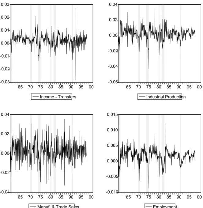
We begin our analysis by considering the coincident series, which are deÞned in Table 1, and are plotted in Figure 1, where shaded areas represent the NBER dating of recession periods. All four series show signs of dropping during recessions, although this behav-ior is more pronounced for Industrial Production (∆lnYt) and Employment (∆lnNt). These two series also show a more visible cyclical pattern, whereas, for example, it is hard to notice the cyclical pattern in Sales (∆lnSt) or Income (∆lnIt). Before modelling the joint cyclical pattern of the coincident series in (∆lnIt, ∆lnYt, ∆lnNt, ∆lnSt), we performed cointegration tests to verify if the series in (lnIt,lnYt,lnNt,lnSt) share a
common long-run component. As in Stock and Watson (1989), weÞnd no cointegration
among these variables.
Conditional on the evidence of no cointegration for the elements of(lnIt,lnYt,lnNt,lnSt),
we model them as a Vector Autoregression (VAR) in Þrst differences. Besides
(∆lnIt, ∆lnYt, ∆lnNt, ∆lnSt) and their lags, the VAR also contains the lags of
9We thank Mark Watson for suggesting this exercise to us. Indeed, he suggested as well that we could
go a step further, choosing the weights of coincident series that would best Þt the NBER’s committee
peaks and troughs. We leave that for future research.
transformed (mostly by log Þrst differences) leading series as a conditioning set. The latter is a sensible choice because we should expect,a priori, that these leading series are helpful in forecasting the coincident series. A list of these leading series is also presented in Table 1. They were used by Stock and Watson(1988a) and comprise a subset of the variables initially chosen by Burns and Mitchell (1946) to be leading indicators11.
The Akaike Information Criterion chose a VAR of order 2. Conditional on aV AR(2)
we calculated the canonical correlations between the coincident series (∆lnIt, ∆lnYt,
∆lnNt, ∆lnSt) and the respective conditioning set, comprising of two lags of (∆lnIt,
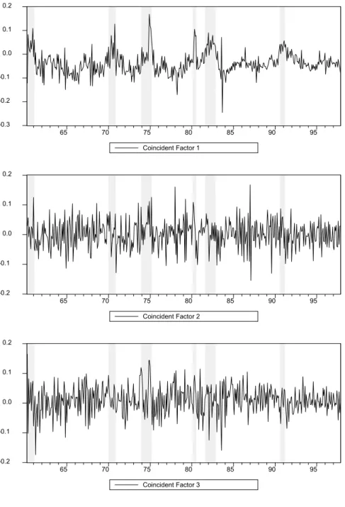
∆lnYt,∆lnNt,∆lnSt) and of two lags of the leading series. The canonical-correlation test results in Table 2 allow the conclusion that there is only one linear combination of the coincident series which is white noise. Hence, the cyclical behavior of (∆lnIt,∆lnYt,
∆lnNt,∆lnSt) can be represented by three orthogonal canonical factors. These factors,
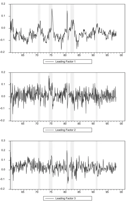
(c1t, c2t, c3t), were labelled as the coincident basis cycles and are a linear combination of the coincident series. A plot of them is presented in Figure 2. Figure 3, on the other hand, presents the estimates of the linear combinations of the leading series in the canonical-correlation analysis, (γ0
1zt,γ02zt,γ03zt), labelled leading factors.
Below, we show the linear combinations of the four coincident indicators that yield the three basis cycles:
c1t c2t c3t
=
1.03 0.31 19.44 −0.68
−1.68 1.12 1.12 4.64
−0.27 7.78 −13.46 −2.33 ×
∆lnIt
∆lnYt
∆lnNt
∆lnSt
(6)
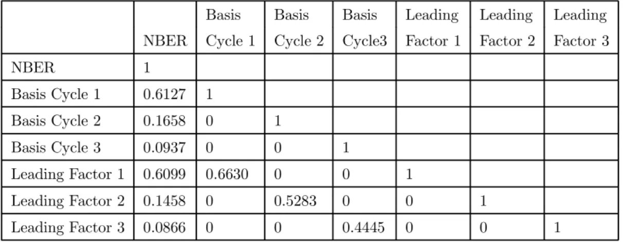
A correlation matrix for all six (coincident and leading) factors is presented in Table 3. To investigate their ability in explaining NBER recessions we include in this correlation matrix the NBER recession indicator dummy (which is equal to one during periods
identiÞed by NBER as recessions and zero otherwise). As could be expected a priori,
theÞrst factor (either coincident or leading) is the one with the highest correlation with
the NBER dummy variable, followed by the second, andÞnally by the third.
3.2 “The Missing Link”: using the NBER information in computing the coincident index
The structural model in (3) enables us to incorporate the information in the NBER recession indicator in constructing a coincident index of economic activity. It also incor-porates the information resulted from the canonical correlation analysis, namely that there are only three signiÞcant basis cycles in the four coincident series. We use the two stage conditional maximum likelihood (2SCML) estimator proposed by Rivers and
11Stock and Watson smooth some of these leading indicators. Here, we make no use of such
Vuong (1988) to obtain instrumental variable estimates for the coefficients of each basis cycle.
The 2SCML estimates are presented in Table 4. After rewriting the basis cycles as linear combinations of the coincident series and normalizing the weights to add up to unity, we obtain our index, which we call the instrumental-variable coincident index
(IV CIt):
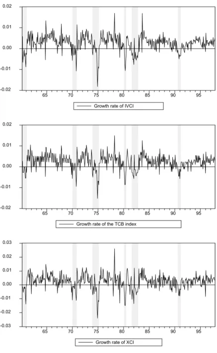
∆IV CIt= 0.02×∆lnIt+ 0.13×∆lnYt+ 0.80×∆lnNt+ 0.05×∆lnSt. (7)
Equation (7) shows that most of the weight is given to employment, and that em-ployment and industrial production together get 93% of the weight. A plot of this index is presented in Figure 4. This is not surprising given our previous analysis of Figure 1, since these two series have a more pronounced coherence with the NBER recession indicator. It also agrees with the latest memo of the Business Cycle Dating Committee (Hall et al. 2002, p. 9) where they state “employment is probably the single most reliable indicator [of recessions]”. It is interesting to compare our index with alternative indices in the literature. The corresponding weights that are used by the Conference Board to calculate the coincident index12 are(0.28,0.13,0.48,0.11).The striking diff
er-ence between our weights and those of the TCB index is that income (It) is weighed
much more heavily in the TCB index than in ours, and employment (Nt) is weighed
more heavily in our index than in theirs.
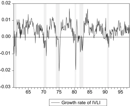
Finally, as a by-product of this analysis, we can construct a leading index, which uses the same weights estimated by instrumental-variable probit and the leading fac-tors (γ0
1zt,γ02zt,γ03zt) weighed by their respective canonical correlations. This index is labelled ∆IV LIt and is presented in Figure 5. It must be emphasized that this is only a one step-ahead leading index. In order to create several step-ahead leading indices, our model must be enlarged to include forecasting equations for the leading variables in zt. Since best forecasting equations for some of the leading variables (such as interest
rates) are nonlinear, we believe that proper several step-ahead leading indices cannot be linear. However, the construction of such indices is beyond the scope of the present paper.
3.3 Comparisons with Existing Coincident Indices
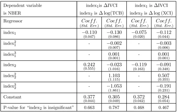
We perform the speciÞcation tests described in Section 2.3 regarding the TCB index and
the experimental index13 (XCI) proposed by Stock and Watson (1989). The results of
estimating equations (4) and (5), once with the TCB index and once with the XCI index as the alternative index, are presented in Table 5. This table also shows the p-values
12The Conference Board Index is also known as the Department of Commerce Index (or the DOC
Index).
of the null hypothesis of “given our index, the alternative index is insigniÞcant” in each equation. It can be seen from this table that the coefficients of our index are signiÞcant, whereas there is no evidence that the coefficients of the other two indices are signiÞcantly different from zero. The results of these tests clearly indicate that, controlling for our index, there is no useful information in either the TCB or the XCI indices in explaining the business cycle state of the economy.
We have labelled this a speciÞcation test since our coincident index models directly the state of the economy, as decided by the NBER Business Cycle Dating Committee, whereas the other two indices do not. To implement a more “neutral” test for these three coincident indices, we decided to measure how useful each of them is in describing the actual peaks and troughs of U.S. economic activity. As discussed at the end of Section 2.3, we verify their relative success in this task by measuring the peaks and troughs of economic activity implied by their time-series behavior, comparing the results with peaks and troughs implied by the NBER Dating Committee’s decisions.
We use the Bry and Boschan (1971) algorithm to extract peaks and troughs of all three indices, and confront the results with the actual NBER Dating Committee’s decisions using a quadratic loss function. The results show that our index, IVCI, has the smallest loss function overall: 0.028 versus 0.032 for the next index, and 0.041 for the last one. Hence, IVCI has a 2.8% chance of erroneously classifying the state of the economy in sample, which is better than the performance of other existing coincident indices.
The reason for the performance of IVCI can be analyzed by looking closely at speciÞc boom and recession episodes. Our index makes its largest error in missing the onset of the 1973 recession from 12/1973 through 7/1974. However, IVCI outperforms the TCB and XCI indices in several occasions where these two indices give a false alarm of a recession. The single most important of such episodes occurred during the period 8/1980 through 7/1981. It is worth noticing that XCI produces the largest number of false alarms of a recession among the three indices. A possible explanation for the favorable behavior of IVCI is the fact that our index places a larger weight on employment relative to the
other two. Because there are costs in hiring and Þring employees, employment may
4
Conclusion
The basic idea behind this paper is simple: use the information content in the NBER Business Cycle Dating Committee decisions to construct a coincident index of economic activity. Although several authors have devised sophisticated coincident indices with the ultimate goal of matching NBER recessions, no one has used the information in the NBER decisions to construct a coincident index. The second ingredient of our method is that we use canonical correlation analysis toÞlter out the noisy information contained in the coincident series. As a result, our Þnal index is only inßuenced by the cyclical components of the coincident series. In our model, a structural equation relates the unobserved state of the economy to the cyclical components of the coincident series. We use a two stage conditional maximum likelihood method to use the information in the NBER recession indicator about the unobserved state of the economy in order to estimate the parameters of this structural equation. The resulting index is a simple linear combination of the four coincident series originally proposed by Burns and Mitchell (1946).
As explained in the Introduction, we like to think that our method uncovers the “Missing Link” between the pioneering research of Burns and Mitchell (1946) and the deliberations of the NBER Business-Cycle Dating Committee. This is a consequence of the way we have constructed our coincident index: the coincident index is a linear com-bination of the four coincident series proposed by Burns and Mitchell that has a common cycle with an unobserved state variable which is consistent with the deliberations of the NBER Business Cycle Dating Committee. It is noteworthy that our coincident index places the largest weight on employment (80%), which is in agreement with the latest opinion of the NBER Business Cycle Dating Committee (Hall et al. 2002, p. 9) that “employment is probably the single most reliable indicator [of recessions]”.
Our methodology also conveniently produces a one-step leading index of economic activity which is a linear combination of lags of coincident and leading variables. More-over, the probit model that produces our coincident index is in fact a model of probability of recessions. Therefore, this model can easily produce estimates of the probability of a recession.
The performance of our constructed coincident index is promising. With speciÞ
ca-tion tests against particular alternatives, we conclude that there is no gain in combining our index with either of the two currently popular coincident indices, namely the TCB and the XCI coincident indices. This means that given our index, there is no useful information in the other two indices about the state of the economy. Although techni-cally we cannot conclude that our index encompasses the TCB and XCI indices, because those two indices do not use the information in the NBER dates in their construction,
the speciÞcation test results delineate the important question that motivated our
construction?
In countries where there are no institutions similar to the NBER Business Cycle Dating Committee, simple rules such as two quarters of negative growth in the GDP or the quarterly version of Bry and Boschan (1971) algorithm applied to the quarterly GDP are used to identify recessions. A useful extension of the present paper will be to use our structural framework to identify the coincident index as the common cycle between the monthly coincident variables and the quarterly recession indicator or the quarterly GDP series. This extension is left for future research.
References
Akaike, H. (1976), “Canonical Correlation Analysis of Time Series and the Use of an
Information Criterion”, in R.K. Mehra and D.G. Lainiotis (Eds) System IdentiÞ
-cation: Advances and Case Studies, New York: Academic Press, pp. 27-96.
Anderson, T. W. (1984), An Introduction to Multivariate Statistical Analysis (2nd
ed.). NewYork: John Wiley and Sons.
Anderson, H. M. and F. Vahid (1998), “Testing Multiple Equation Systems for
Com-mon Nonlinear Factors”, Journal of Econometrics,84, 1-37.
Balke, N.S. and T.B. Fomby (1997), “Threshold Cointegration”, International
Eco-nomic Review, 38, 627-647.
Bry, G. and C. Boschan (1971),Cyclical Analysis of Time Series: Selected Procedures
and Computer Programs, New York: NBER.
Burns, A. F. and Mitchell, W. C.(1946),Measuring Business Cycles. New York:
Na-tional Bureau of Economic Research.
Chauvet, M. (1998), “An Econometric Characterization of Business Cycle Dynamics
with Factor Structure and Regime Switching”, International Economic Review,
39, 969-996.
Davidson, R. and MacKinnon, J.G. (1993), “Estimation and Inference in Economet-rics,” Oxford: Oxford University Press.
Engle, R. F. and Kozicki, S. (1993), “Testing for Common Features”, Journal of
Business and Economic Statistics, 11, 369-395, with discussions.
Engle, R. F. and Issler, J. V. (1995), “Estimating Sectoral Cycles Using Cointegration
and Common Features”, Journal of Monetary Economics, 35, 83-113.
Estrella A. and F. S. Mishkin (1998), “Predicting U.S. Recessions: Financial Variables
Geweke, J. (1977), “The Dynamic Factor Analysis of Economic Time Series,” Chapter
19 in D.J. Aigner and A.S. Goldberger (eds) Latent Variables in Socio-Economic
Models, Amsterdam: North Holland.
Hall, R., Feldstein, M., Bernanke, B., Frankel, J., Gordon, R. and Zarnowitz, V. (2002), “The NBER’s Business-Cycle Dating Procedure”, downloadable from http://www.nber.org/cycles/recessions.pdf.
Hamilton, J.D. (1994),Time Series Analysis, Princeton: Princeton University Press.
Hamilton, J.D. (1989), “A New Approach to the Economic Analysis of Nonstationary
Time Series and the Business Cycle”,Econometrica, 57, 357-384.
Harding, D. and A.R. Pagan (2002), “Dissecting the Cycle: A Methodological
Inves-tigation”, Journal of Monetary Economics, 49, 365-381.
Hecq, A., F. Palm and J.P. Urbain (2000), “Permanent-Transitory Decomposition in
VAR Models with Cointegration and Common Cycles”, Oxford Bulletin of
Eco-nomics and Statistics, 62, 511-532.
Hotelling, H. (1935), “The Most Predictable Criterion”,Journal of Educational
Psy-chology, 26, 139-142.
Hotelling, H. (1936), “Relations Between Two Sets of Variates”,Biometrika, 28, 321-377.
Issler, J.V. and Vahid, F. (2001), “Common Cycles and the Importance of Transitory
Shocks to Macroeconomic Aggregates,”Journal of Monetary Economics, 47,
449-475.
Lahiri, K. and G. Moore (1993), Editors, “Leading Economic Indicators: New
Ap-proaches and Forecasting Records.” New York: Cambridge University Press.
Mizon, G.E. (1984), “The Encompassing Approach in Econometrics”, Chapter 6 in
D.F. Hendry and K.F. Wallis (eds) Econometrics and Quantitative Economics,
Oxford: Blackwell.
Newey, W. and K. West (1987), “A Simple Positive Semi-DeÞnite, Heteroskedasticity
and Autocorrelation Consistent Covariance Matrix,” Econometrica, 55, 703-708.
Rivers, D. and Q.H. Vuong (1988), “Limited Information Estimators and Exogeneity
Tests for Simultaneous Probit Models”, Journal of Econometrics, 39, 347-366.
Stock, J. and Watson, M.(1988b), “A Probability Model of the Coincident Economic Indicator”, NBER Working Paper # 2772.
Stock, J. and Watson, M.(1989) “New Indexes of Leading and Coincident Economic
Indicators”, NBER Macroeconomics Annual, pp. 351-95.
Stock, J. and Watson, M.(1991), “A Probability Model of the Coincident Economic
Indicators”, in “Leading Economic Indicators: New Approaches and Forecasting
Records,” K. Lahiri and G. Moore, Eds. New York: Cambridge University Press.
Stock, J. and Watson, M.(1993a), “A Procedure for Predicting Recessions with
Lead-ing Indicators: Econometric Issues and Recent Experiences,” in “New Research
on Business Cycles, Indicators and Forecasting,” J.H. Stock and M.W. Watson, Eds., Chicago: University of Chicago Press, for NBER.
Stock, J. and Watson, M.(1993b), Editors, “New Research on Business Cycles, Indi-cators and Forecasting” Chicago: University of Chicago Press, for NBER.
The Conference Board (1997), “Business Cycle Indicators,” Mimeo, The Conference Board, downloadable from http://www.tcb-indicators.org/bcioverview/bci4.pdf.
Vahid, F. and Engle, R. F. (1993), “Common Trends and Common Cycles”,Journal
of Applied Econometrics, 8, 341-360.
Vahid, F. and Engle, R.F.(1997), “Codependent Cycles,”Journal Econometrics, vol.
80, pp. 199-121.
Watson, M.W. (1994), “Business-Cycle Durations and Postwar Stabilization of the
U.S. Economy,” American Economic Review, 84, 24-46.
Wooldridge, J.M.(1994), “Estimation and Inference for Dependent Processes,” in “Handbook of Econometrics IV,” R.F. Engle and D. McFadden, Editors. Ams-terdam: Elsevier Press.
A
Econometric and statistical techniques
A.1 Statistical foundation of TCB and XCI indices
A coincident index, which is widely used by practitioners, is the index constructed by The Conference Board — TCB. This coincident index is a weighted average of the coincident variables — employment, output, sales and income, where weights are the reciprocal of the standard deviation of each component’s growth rate and add up to unity; see The Conference Board (1997).
Stock and Watson’s experimental coincident index(XCI)is based on an “unobserved
growth rate of the four coincident series (output, sales, income and employment) share a common cycle,∆XCIt, which is a latent dynamic factor that represents (the change
of) “the state of the economy.” Denoting the growth rates of the coincident series in a vectorxt= (x1t, x2t, x3t, x4t)
0
, their proposed statistical model is as follows:
xt = β+γ(L)∆XCIt+ut,
φ(L)∆XCIt = δ+ηt,
D(L)ut = ²t, (8)
whereφ(L)andγ(L)are scalar polynomials on the lag operatorL, andD(L)is a matrix
polynomial onL. The error structure is restricted so as to haveE
à ηt ²t ! à ηt ²t !0
=
diag(σ2η,σ2²1, ...,σ2²4), andD(L) =diag[dii(L)], which makes innovations mutually uncor-related.
The model (8) assumes that there is a single source of comovement among the growth rates of the coincident series — ∆XCIt. Still, these series are allowed to have their own idiosyncratic cycle, since the vector of error terms ut is composed of serially correlated components that are mutually orthogonal. Hence, each of the four coincident series in
xt has two cyclical components: a common and an idiosyncratic one. In this view, the
“business cycle” is the intersection of the cycles in output, income, employment, and
trade. Moreover, there is no guarantee that idiosyncratic cycles do not dominate the common cycle in explaining the variation of the four series in xt.
In contrast, in our view, the “business cycle” is theunion of the cycles in output, income, employment, and trade. There are no idiosyncratic cycles that can be put aside, the only part ofxtthat we leave out is the non-cyclical combination resulting from the canonical-correlation analysis. Comparing our method with Stock and Watson’s clearly shows that neither model is a special case of the other. Hence, neither model is nested within the other one, and comparisons between them have to be made using non-nested tests. Chauvet (1998) has generalized the framework in Stock and Watson by allowing
a two-state mean for the latent factor ∆XCIt in (8), representing recession and
non-recession regimes.
A.2 Canonical correlations
Consider two (stationary) random vectorsx0
t= (x1t, x2t, ..., xnt)andzt0 = (z1t, z2t, ..., zmt),
m≥nsuch that: µ
xt zt ¶ ∼ µµ 0 0 ¶ , µ
ΣXX ΣXZ
ΣZX ΣZZ
¶¶ .
A0 (n×n)=
α0 1 α0 2 .. . .. . α0 n
and Γ0
(n×m)= γ0 1 γ0 2 .. . .. . γ0 n such that:
1. The elements ofA0
xt have unit variance and are uncorrelated with each other:
E(A0
xtx0tA) =A 0
ΣXXA=In
2. The elements ofΓ0
zt have unit variance and are uncorrelated with each other:
E(Γ0ztz 0 tΓ) =Γ
0
ΣZZΓ=In, and,
3. The i-th element ofA0x
t is uncorrelated with thej-th element of Γ0zt,i6=j. For i=j, this correlation is a called canonical correlation, denoted byλi, such that:
E(A0xtz 0
tΓ) =A 0
ΣXZΓ=Λ,
where, Λ=
λ1 0 · · · 0 0 λ2 0 · · · 0
..
. . .. ...
..
. . .. 0
0 · · · 0 λn
, and,
1≥|λ1|≥|λ2|≥...≥|λn|≥0.
The following basic results in Anderson (1984) and Hamilton (1994) are worth reporting here.
Proposition 1 The k-th canonical correlation between xt andztis given by k-th highest
root of ¯ ¯ ¯ ¯ ¯
−λΣXX ΣXZ
ΣZX −λΣZZ
¯ ¯ ¯ ¯
¯ = 0, denoted by λk. The linear combinations αk and γk associated withà λk can be found by making λ=λk in
−λΣXX ΣXZ
ΣZX −λΣZZ
! Ã αk
γk !
= 0, considering also the unit-variance restrictions
Proposition 2 LetX= (x1,x2, ..., xT)0 andZ= (z1, z2, ..., zT)be samples ofT observa-tions of xt andzt. The n Þrst eigenvalues of the matrixH= (X0X)−1X0Z(Z0Z)−1Z0X are consistent estimates of the squared populational canonical correlations(λ21,λ22, ...,λ2n). The corresponding eigenvectors are consistent estimates of the parameters in A.
More-over, the Þrst n eigenvalues of H are identical to the Þrst n eigenvalues of the matrix
G = (Z0
Z)−1Z0 X(X0
X)−1X0
Z, whose corresponding eigenvectors are consistent
esti-mates of the elements of Γ.
Proposition 3 The likelihood ratio test statistic for the null hypothesis that the smallest
n−k canonical correlations are jointly zero, Hk :λk+1 = λk+2 = ...=λn = 0, can be computed using the squared sample canonical correlations bλ2i, i =k+1,· · · , n, in the following fashion:
LR=−T n X
i=k+1
ln(1−λb2i).
Moreover, the asymptotic distribution of this likelihood-ratio test statistic is chi-squared,
as follows:
LR−→d χ2(n−k)(m−k).
Canonical-correlation analysis can be applied in the present context for analyzing a large multivariate data set, summarizing the correlations between a group of stationary series xand a group of stationary seriesz. For example, we suppose that the coincident
series in xt can be modelled using a Vector Autoregression (VAR), using its own the
lags, xt−1,· · ·, xt−p, and also the lags of some other (leading) series,wt−1,· · ·, wt−p, as
follows:
xt=A1xt−1+· · ·+Apxt−p+B1wt−1+· · ·+Bpwt−p+εt, (9) whereεt is a white-noise process.
Here, we are interested in summarizing the correlations between the variables in xt and the variables in zt =
¡ x0
t−1,· · ·, x 0 t−p, w
0
t−1,· · ·, w 0 t−p
¢0
. In this framework, the cyclicalfeatureinxthas to arise from the elements inzt, sinceεtis a white-noise process, devoid of any cyclical features; see Engle and Kozicki(1993).
A.3 Two stage conditional maximum likelihood estimation
Denoting by c1t,· · · , ckt, (cit =α0ixt, i=1,· · ·, k), the k basis cycles associated with the Þrst knon-zero canonical correlations, the NBER business-cycle indicator is linked to them through the latent variabley∗
t:
E(yt∗ | It+h) =β0+β1c1t+· · ·+βkckt+ut (10)
NBERt =
(
1 ifE(y∗
t |It+h)<0
The possible correlation betweenc1t,· · ·, ckt and the errors ut is modelled as follows,
cit = λi ¡
γ0izt ¢
+vit, i=1,· · · , k (11) Ã ut vt ! ∼ N Ã 0, "
σ2u σ0 vu σvu Σvv
#!
where the vit,i=1,· · ·, k, are collected into a k-vector vt,λi and γ0izt fori=1,· · · , k come from the canonical-correlation analysis,Σvvis ak×kdiagonal variance-covariance matrix of vt, σvu is a k×1 vector of covariances between ut and vt. Because of mea-surement error, the basis cyclesc1t,· · · , cktare correlated withut. Joint normality ofut and vt implies:
ut=v 0 tδ+ηt
whereδ=Σ−1
vvσvu,ηt∼N ¡
0,σ2u−σ0
vuΣ−vv1σvu ¢
andηtis independent ofvt.Substituting forut in equation (10), we obtain,
E(y∗
t | It+h) =β0+β1c1t+· · ·+βkckt+v0tδ+ηt (12)
NBERt =
(
1 ifηt<−(β0+β1c1t+· · ·+βkckt+vt0δ)
0 ifηt≥ −(β0+β1c1t+· · ·+βkckt+vt0δ) .
Notice that, by construction, all the regressors in (12) are uncorrelated with the error term ηt. As usual for probit models the mean parameters θ =¡β0,β1,β2,β3,δ0¢0
and the variance parameter ¡σ2η =σ2u−σ0
vuΣ−vv1σvu ¢
are not separately identiÞable. The
convenient normalization σ2η = 1 will identify the mean parameters. Obtaining the
two stage conditional maximum likelihood (2SCML) estimator proposed by Rivers and Vuong (1988) entails the following steps:
1. Regress cit,i=1,· · · , k, on ztto get bvit andΣbvv, a consistent estimate ofΣvv.
2. From bvit, i= 1,· · · , k, form bvt and then run a probit regression (12) to get con-sistent estimates ofθ=¡β0,β1,β2,β3,δ0¢0, denoted by bθ.
For inference onθ, ifηt is i.i.d., the following central-limit theorem holds: √
T³bθ−θ´−→d N(0, V),
where the appropriate formula for the asymptotic covariance matrixV is given in Rivers
and Vuong(1988, p. 354).
B
Tables and
Þ
gures
Table 1: Coincident and Leading Series: DeÞnitions and Transformations
Series DeÞnition Transformation
Coincident Series
INDUSTRIAL PRODUCTION: TOTAL INDEX (1992=100,SA) —Yt ∆ln (·) EMPLOYEES ON NONAG. PAYROLLS: TOTAL (THOUS.,SA) —Nt ∆ln (·) MANUFACTURING & TRADE SALES (MIL$, 92 CHAINED $) —St ∆ln (·) PERS. INCOME LESS TRANSF. PMTS. (CHAINED, BIL 92$,SAAR) — It ∆ln (·) Leading Series
MFG UNFIL.ORD.: DUR.GOODS IND., TOT.(82$,SA) = MDU/PWDMD ∆ln (·)
MANUFACT. & TRADE INVENT.:TOTAL (MIL OF CHAINED 1992, SA) ∆ln (·)
NEW PRIV. OWNED HOUSING: UNITS AUTH. BUILD. PERMITS SAAR ∆ln (·)
IND. PRODUCTION: DURABLE CONSUMER GOODS (1992=100,SA) ∆ln (·)
INT. RATE: U.S.TRS. CONST MATUR.,10-YR.(% PER ANN,NSA) ∆(·)
INT. RATE SPREAD = 3 MONTHS - 10 YEARS (FYGM3-FYGT10) NONE NOMINAL WEIGHTED EXCHANGE RATE OF G7 (EXCL. CANADA) ∆ln (·)
EMPLOYEES ON NONAG. PAYROLLS: SERVICE-PROD.(THOUS.,SA) ∆ln (·)
Table 2: Squared Canonical Correlations and Canonical-Correlation Test
Sq. Canonical Correlations Degrees of Freedom λ2j and all smaller λ2j = 0
λ2j P-Values
0.4397 104 0.0000
0.2791 75 0.0000
0.1976 48 0.0000
0.0654 23 0.1332
Table 3: Correlation Matrix for Factors and NBER Recession-Indicator
Basis Basis Basis Leading Leading Leading NBER Cycle 1 Cycle 2 Cycle3 Factor 1 Factor 2 Factor 3
NBER 1
Basis Cycle 1 0.6127 1
Basis Cycle 2 0.1658 0 1
Basis Cycle 3 0.0937 0 0 1
Leading Factor 1 0.6099 0.6630 0 0 1
Leading Factor 2 0.1458 0 0.5283 0 0 1
Table 4: Two Stage Conditional Maximum Likelihood Estimates
Regressor Est. Coeff. Std. Error
c1t 75.13 10.71
c2t 32.56 7.45
c3t 14.01 8.27
Constant -0.15 0.23
Table 5: SpeciÞcation Test Results
Dependent variable index1is∆IVCI index1 is∆IVCI is NBER index2 is∆log(TCB) index2 is∆log (XCI)
Regressor Coef f.
(Std. Err.)
Coef f. (Std. Err.)
Coef f. (Std. Err.)
Coef f. (Std. Err.)
index1 −0.110
(0.047) −0 .130
(0.086) −0 .075
(0.020) −0 .112 (0.044)
index21 - −0.002
(0.007)
- −0.003 (0.006)
index31 - 0.001
(0.001) - (00..00001)1
index2 0.242
(0.555) −(10..016)023 −0 .119
(0.163) −0 .091
(0.348)
index22 - 1.103
(1.115) - (00..507355)
index32 - −1.053
(1.861) - −0 .191
(0.231)
Constant 0.377
(0.044) (00..305049) (00..372042) (00..284054) P-value for “index2 is insigniÞcant” 0.663 0.787 0.468 0.467
In both tables, all equations are estimated using 2 lags of coincident and leading variables as
instruments. The standard errors and p-values are calculated using the Newey-West estimator of the
-0.03 -0.02 -0.01 0.00 0.01 0.02 0.03
65 70 75 80 85 90 95 00
Income - Transfers
-0.06 -0.04 -0.02 0.00 0.02 0.04
65 70 75 80 85 90 95 00
Industrial Production
-0.04 -0.02 0.00 0.02 0.04
65 70 75 80 85 90 95 00
Manuf. & Trade Sales
-0.010 -0.005 0.000 0.005 0.010 0.015
65 70 75 80 85 90 95 00
Employment
-0.3 -0.2 -0.1 0.0 0.1 0.2
65 70 75 80 85 90 95 Coincident Factor 1
-0.2 -0.1 0.0 0.1 0.2
65 70 75 80 85 90 95 Coincident Factor 2
-0.2 -0.1 0.0 0.1 0.2
65 70 75 80 85 90 95 Coincident Factor 3
-0.2 -0.1 0.0 0.1 0.2
65 70 75 80 85 90 95 00 Leading Factor 1
-0.2 -0.1 0.0 0.1 0.2
65 70 75 80 85 90 95 00 Leading Factor 2
-0.2 -0.1 0.0 0.1 0.2 0.3
65 70 75 80 85 90 95 00 Leading Factor 3
-0.02 -0.01 0.00 0.01 0.02
65 70 75 80 85 90 95 Growth rate of IVCI
-0.02 -0.01 0.00 0.01 0.02
65 70 75 80 85 90 95 Growth rate of the TCB index
-0.03 -0.02 -0.01 0.00 0.01 0.02 0.03
65 70 75 80 85 90 95 Growth rate of XCI
-0.03 -0.02 -0.01 0.00 0.01 0.02
65 70 75 80 85 90 95
Growth rate of IVLI