Funda¸c˜
ao Getulio Vargas
Ensaios em Econometria Aplicada
Tese de submetida `a Escola de P´os-Gradua¸c˜ao em Economia da Funda¸c˜ao
Getulio Vargas como quesito para a obten¸c˜ao T´ıtulo de Doutor em Economia.
Aluno: Rafael Martins de Souza
Orientador: Jo˜ao Victor Issler
Rio de Janeiro
Escola de P´
os-Gradua¸c˜
ao em Economia - EPGE
Funda¸c˜
ao Getulio Vargas
Ensaios em Econometria Aplicada
Tese de submetida `a Escola de P´os-Gradua¸c˜ao em Economia da Funda¸c˜ao
Getulio Vargas como quesito para a obten¸c˜ao T´ıtulo de Doutor em Economia.
Aluno: Rafael Martins de Souza
Banca Examinadora:
Jo˜ao Victor Issler (Orientador, EPGE/FGV)
Prof. Marco Antonio Bonomo (EPGE/FGV)
Caio Ibsen Rodrigues de Almeida (EPGE/FGV)
Marcelo C. Medeiros (DE/PUC-Rio)
Paulo Pichetti (EESP/FGV)
Rio de Janeiro
Abstract
This thesis has three chapters. Chapter 1 explores literature about exchange rate pass-through,
approaching both empirical and theoretical issues. In Chapter 2, we formulate an estate space
model for the estimation of the exchange rate pass-through of the Brazilian Real against the US
Dollar, using monthly data from August 1999 to August 2008. The state space approach allows us
to verify some empirical aspects presented by economic literature, such as coefficients inconstancy.
The estimates offer evidence that the pass-through had variation over the observed sample. The
state space approach is also used to test whether some of the “determinants” of pass-through are
related to the exchange rate pass-through variations observed. According to our estimates, the
variance of the exchange rate pass-through, monetary policy and trade flow have influence on the
exchange rate pass-through. The third and last chapter proposes the construction of a coincident
and leading indicator of economic activity in the United States of America. These indicators
are built using a probit state space model to incorporate the deliberations of the NBER Dating
Cycles Committee regarding the state of the economy in the construction of the indexes. The
estimates offer evidence that the NBER Committee weighs the coincident series (employees in
non-agricultural payrolls, industrial production, personal income less transferences and sales) differently
way over time and between recessions. We also had evidence that the number of employees in
non-agricultural payrolls is the most important coincident series used by the NBER to define the periods
iv
Resumo
A tese est´a dividida em trˆes cap´ıtulos. O cap´ıtulo 1 trata de uma revis˜ao de literatura sobre
pass-through, abordando aspectos emp´ıricos e te´oricos. O segundo cap´ıtulo trata da estima¸c˜ao de
um modelo de espa¸co de estados para estima¸c˜ao dos pass-through da taxa de cˆambio no Brasil de
agosto 1999 a agosto 2008. A abordagem espa¸co de estados permite contemplar alguns aspectos
emp´ıricos apresentados pela literatura econˆomica, tais como a inconstˆancia dos parˆametros. As
estimativas ofereceram evidˆencia de que o pass-through no Brasil variou no per´ıodo estudado.
Ainda, a abordagem por espa¸co de estados permite que se estude os“determinantes” (ou vari´aveis
associadas) do pass-through. Com isto tivemos evidˆencia de que a variˆancia da taxa de cˆambio, a
pol´ıtica monet´aria e o fluxo de com´ercio afetam o pass-through. O terceiro e ´ultimo artigo da tese
trata da constru¸c˜ao de um indicador coincidente e antecedente da atividade econˆomica nos Estados
Unidos da Am´erica. Nele utiliza-se um modelo probit de espa¸co de estados para incorporar as
decis˜oes do NBER Dating Cycles Committee na constru¸c˜ao dos ´ındices. A estimativas ofereceram
evidˆencia de que o comitˆe do NBER pondera as s´eries coincidentes (total de empregados em
atividades n˜ao agr´ıcolas, produ¸c˜ao industrial, renda pessoal menos transferˆencias governamentais
e vendas) de maneira diferente ao longo do tempo e entre as recess˜oes. Tamb´em evidenciou-se que
a s´erie coincidente total de empregados em setores n˜ao-agr´ıcolas ´e a principal s´erie considerada
Agradecimentos
Agrade¸co,
A Deus, por me permitir caminhar at´e aqui, apesar de todas as dificuldades.
Ao meu orientador, Prof. Jo˜ao Victor Issler pelo apoio, incentivo e exemplo profissional. Ao
Prof. Pedro Cavalcanti Gomes Ferreira que abriu as portas da EPGE quando eu era, ainda, um
aluno de gradua¸c˜ao para fazer bolsa de inicia¸c˜ao cient´ıfica.
`
A Funda¸c˜ao Getulio Vargas, `a CAPES e ao CNPq pelo suporte financeiro.
Aos amigos de San Diego, Daniel, Daniel Aiex e Eillen. O conv´ıvio com vocˆes foi inesquec´ıvel.
A gratid˜ao ´e eterna.
A todos os amigos da EPGE. Em especial ao Jos´e Diogo, ao Orlando, ao James, ao Fl´avio,
ao Luiz Felipe, `a Amanda, ao Pedro, ao Gustavo, ao Gabriel e ao Hilton. Obrigado por todos os
momentos.
Aos meus amigos de longa data, Aline e Ralph, que, mesmo quando estavam em pa´ıses distantes,
estivem sempre pr´oximos o suficente para me encorajar e me incentivar nos momentos dif´ıcies.
Aos meus novos colegas de trabalho, Luisa e Gustavo, que pela paciˆencia, incentivo e for¸ca na
reta final.
Aos meus pais, Marlene e Ronaldo, e ao meu irm˜ao Samuel, por todo amor, incentivo,
encora-jamento, participa¸c˜ao... Descrever toda a importˆancia da nossa fam´ılia ´e imposs´ıvel. A gratid˜ao ´e
infinita.
`
A Mozuca, pela sua paciˆencia, benevolˆencia, altru´ısmo, seu trato carinhoso, sua calma, sua
vi
Key words and phrases: Exchange rate pass-through, business cycles, indicators of economic
activity, state space models, Kalman filter.
Palavras-Chave: Pass-throughda taxa de cˆambio, ciclo de neg´ocios, indicadores de atividade
Contents
I
Exchange Rate Pass-Through
1
1 A Discussion on Exchange Rate Pass-Through 2
1.1 Introduction . . . 2
1.2 Empirical Evidences on Exchange Rate Pass-Through . . . 4
1.3 Pass-Through Determinants . . . 8
1.3.1 Macroeconomic Determinants . . . 8
1.3.2 Output Gap . . . 8
1.3.3 Microeconomic Determinants of Pass-Through . . . 11
1.4 The economic model . . . 12
2 Pass-Through Estimation in Brazil 15 2.1 Introduction . . . 15
2.2 Econometric Framework . . . 16
2.2.1 Linear state space models under restrictions . . . 16
2.2.2 Model Selection and Inference . . . 19
2.3 Econometric Setting and Estimation . . . 19
CONTENTS viii
2.3.1 Time Varying Coefficients . . . 19
2.3.2 Determinants . . . 30
2.4 Conclusions . . . 35
II
Coincident and Leading Indexes of Economic Activity
37
3 A State Space Model for Indices of Economic Activity 38 3.1 Introduction . . . 383.2 The model . . . 41
3.2.1 Determining a basis for the cyclical components of coincident variables . . . 41
3.2.2 Estimating a structural equation for the unobserved business cycle state . . 43
3.2.3 The iterated extended Kalman filter and smoother . . . 49
3.2.4 The Kalman Filter and Smoother Instrumental Variables Index . . . 51
3.3 Results . . . 54
3.3.1 The Data . . . 54
3.3.2 The Basis Cycles . . . 54
3.3.3 Estimates . . . 57
3.3.4 Predicting Recessions in Real Time . . . 65
List of Figures
2.1 IPA-OG smoothed coefficient of Δ log𝑒𝑡, Δ log𝑒𝑡−1 and Δ log𝑦𝑡−1. . . 25
2.2 IPA-OGPA smoothed coefficient of Δ log𝑒𝑡, Δ log𝑒𝑡−1and Δ log𝑦𝑡−1. . . 26
2.3 IPA-OGPI smoothed coefficient of Δ log𝑒𝑡, Δ log𝑒𝑡−1(top), Δ log𝑦𝑡−1and Δ log𝑦𝑡−6 (bottom). . . 27
2.4 IPA-OG long run pass-through. . . 28
2.5 IPA-OGPA long run pass-through. . . 28
2.6 IPA-OGPI long run pass-through. . . 29
2.7 Tested determinants of pass-through: Monetary policy, (solid line), variance of ex-change rate (dashed line) and international trade (dotted line). . . 31
3.1 Coincident Series. . . 55
3.2 Coincident Cycles (growth rate) plot. . . 58
3.3 Filtered and Smoothed weights. . . 59
3.4 Predicted and Smoothed probabilities using data from 1960:06 to 2007:03. . . 61
3.5 Predicted and Smoothed probabilities using data from 1960:06 to 2007:03. . . 63
3.6 Filtered and Smoothed weights. . . 64
LIST OF FIGURES x
3.7 1990 Recession. . . 66
3.8 2001 Recession. . . 67
List of Tables
2.1 Some quality of fit statistics of the adjusted models. . . 23
2.2 Information criteria observed values for incomplete, null and complete pass-through exchange rate models. . . 24
2.3 P-values of the tests for null and complete pass-through exchange rate. . . 24
2.4 Estimates of the IPA-OG, IPA-OGPA and IPA-OGPI series (p-values between paren-thesis). . . 30
2.5 Estimated parameters and corresponding p-values (in parenthesis). . . 34
2.6 Estimated parameters and corresponding p-values (in parenthesis). . . 34
3.1 Coincident and leading variables. . . 56
3.2 Squared canonical correlations and canonical-correlation test. . . 57
3.3 Descriptive statistics of the filtered (left) and smoothed (right) coefficients. . . 60
3.4 Accuracy of estimation based on a cut-off point of 0.5. . . 62
3.5 Descriptive statistics of the smoothed weights. . . 65
3.6 Predicted probabilities associated for period from 2007:08 to 2008:07 . . . 69
Part I
Exchange Rate Pass-Through
A Discussion on Exchange Rate
Pass-Through
1.1
Introduction
The exchange rate pass-through degree is the elasticity between exchange rate and domestic prices.
In other words, it is the percentage impact on 1% change in exchange rate into domestic prices.
In an open economy, domestic prices can be affected by external shocks, whether by currency
relative price adjustment or by movements in international supply and demand. The exchange
rate pass-through highlights how sensitive each market is to fluctuations in exchange rate.
The study of exchange rate pass-through has intensified since 1980. The literature focuses on
the behavior of the impact of exchange rate on prices and their determinants. However, the real
motivation for these studies was the study of the Purchase Power Parity Puzzle (PPP). The PPP
CHAPTER 1. A DISCUSSION ON EXCHANGE RATE PASS-THROUGH 3
assumption states that all variation in exchange rate is passed-through into prices. The major
conclusion from empirical studies in the last years is that the PPP is not valid in the short run;
therefore, exchange rate pass-through into prices is less than one. However, there is some evidence
in favor of the validity of PPP on long run.
The pass-through estimation could provide a test for the existence of the purchase power parity.
If the PPP were valid in the long term, the pass-through would be complete and the sum of the
pass-through coefficients would have to sum to one. Otherwise, the long run pass-through would
be incomplete and the effect of variations in exchange rate into prices would be restricted.
The importance of exchange rate pass-through has increased since the adoption of the inflation
targeting regime. Fraga, Goldfajn and Minella (2003) have shown that the problem of having a
high exchange rate pass-through degree is that it implies a greater difficulty for attaining inflation
targets. A greater exchange rate pass-through means that the domestic economy is more sensitive
to external shocks, consequently the impact of exogenous shocks into domestic prices is amplified.
Exchange rate pass-through also seens to affect the inflation forecast. According to Goldfajn
and Werlang (2000), the exchange rate pass-through into prices is directly associated with inflation
forecast error. With a smaller pass-through, the domestic economy is more stable and less affected
by external factors. Therefore, a smaller pass-through means that the difference between inflation
expectations and inflation targets is smaller. In other words, a small pass-through generates a
minor inflation forecast error. Consequently, a small pass-through is associated with a major
transparency of inflation path and a minor volatility in price variations in the economy, rising
social welfare and monetary policy efficiency.
The exchange rate pass-through into prices is one of the main drivers to optimal monetary
inflation volatility is dependent on how sensitive prices are to exchange rate variations. They
begin their argument by explaining that the nature of the trade-off between different exchange
rate regimes is quite different in industrial countries from the trade-off in emerging ones. Using a
DGE Model (Dynamic General Equilibrium Model), they argue that the critical distinction is the
exchange rate pass-through into prices. With very high exchange rate pass-through, policies that
stabilize output require high exchange rate volatility, which implies high inflation volatility. But
with limited or delayed pass-through, this trade-off is less pronounced and a flexible exchange rate
policy that stabilizes output can do so without high inflation volatility.
Another study that emphasizes the importance of exchange rate pass-through in an inflation
targeting regime is that of Fraga, Goldfajn and Minella(2003). They have shown that the problem
of having a high exchange rate pass-through degree is that it implies a greater difficulty for attaining
inflation targets. The larger the exchange rate pass-through, the more sensitive the domestic
economy to external shocks, that is, the impact of exogenous shocks on domestic prices is amplified
by a larger exchange rate pass-through.
1.2
Empirical Evidences on Exchange Rate Pass-Through
A main factor in pass-through estimation is the difficulty of using aggregated data and the known
problem of aggregation bias. This factor favors a disaggregating process for prices, and tries to
capture the exchange rate pass-through for each good or each market. Campa and Goldberg (2005)
present results where estimates are better across industries than across countries with aggregate
data. These authors also say that the major source of pass-through variations are competition
CHAPTER 1. A DISCUSSION ON EXCHANGE RATE PASS-THROUGH 5
across industries. Menon (1996) supports these findings pointing to the aggregation bias, indicating
that disaggregated data provides more accurate estimates and captures the impact of exchange
rates on commodities prices more precisely.
Campa and Goldberg (2005) and Pollard and Coughlin (2005) follow this trend of disaggregated
estimation of pass-through. Their approach permits a more individual analysis for each market,
relating pass-through with market power and degree of competition. This type of analysis allows
more plausible explanations for aggregated pass-through behavior. Campa and Goldberg (2005)
observe that the US has seen a change in composition of certain industries in its import basket.
Industries with a bigger pass-through, such as energy and raw materials, have shown a decrease
in their share in the US imports basket, reducing the aggregate pass-through. The proportion of
tradable and non-tradable goods is important to analyze the aggregate exchange rate pass-through
because tradables are more sensitive to changes in exchange rate than the non-tradables. Therefore,
the greater the share of tradable goods, the higher the exchange rate pass-through.
Some results about pass-through estimation can be seen in Goldberg and Knetter (1997), where
the exchange rate pass-through to US inflation was approximately 50% after 6 months. Campa
and Goldberg (2005) estimate pass-through for 25 OECD countries. They found a pass-through of
26%, in the short term, and 41% in the long term for the US. The average pass-through estimated
for OECD countries in the short and long run was 61% and 77%, respectively.
Sekine (2006) estimated exchange rate pass-through for six developed countries (United States,
Japan, Germany, United Kingdom, France and Italy) by taking into account their time-varying
natures. The author incorporates that characteristic by allowing permanent shifts in pass-through
parameters. He found that pass-through has declined over time in all major industrial countries
estimations.
Calvo and Reinhart (2000) have shown that the pass-through degree of emerging countries is
four times greater than that of developed countries. Additionally, these authors calculate that the
variance of inflation compared with the variation of exchange rate is 43% for emerging countries
and 13% for developed ones.
In the case of the Brazilian economy, there are few studies estimating the exchange rate
pass-through. Belaisch (2003) used a VAR specification controlling for petroleum shocks and estimated
the exchange rate pass-through into IPCA approximately 6% after 3 months. He also estimated
other price indeces and found that the pass-through to IPA (34%) was larger than to IGP (27%),
which is larger than IPCA. Carneiro, Monteiro and Wu (2002) used a non-linear estimation for
pass-through into IPCA, in an attempt to capture possible asymmetries in exchange rate variations
into prices. Their estimate was 6,4%, on average.
Albuquerque and Portugal (2003) used a time varying estimation for the IGP, IPCA and IPA.
They found evidence of time varying pass-through in Brazil, although they used a complicated
period (1980-2002). Their data set was prejudiced by multiple exchange rate regimes, multiple
changes in economic policies and some financial crisis. Their state equation estimates for IPA
were not significant, with the exception of the persistence term. For IPCA, their estimates were
approximately 6% on average. However, since 1995 their exchange rate pass-through to IPCA was
not significantly different from null.
After the estimation of exchange rate pass-through, studies started to explain its behavior and
the reasons for so much variation across countries, across time and across industries. The reasons
could be in the exchange rate pass-through determinants. According to Goldfajn and Werlang
CHAPTER 1. A DISCUSSION ON EXCHANGE RATE PASS-THROUGH 7
exhibit smaller pass-through. Another result is that the exchange rate pass-through changes with
time horizon, reaching its peak at 12 months in the case of Brazil. These authors analyzed four
variables as pass-through determinants: real exchange rate misalignment, initial inflation, output
gap and openness degree. Their results indicate that all variables have important correlations with
exchange rate pass-through, depending on the countries’ characteristics, although real exchange
rate misalignment and inflation environment were the most important.
Inflation is positively correlated to exchange rate pass-through. Empirical evidence suggests
that the larger the inflation persistence, the larger inflation rate. Hence, there is more volatily in
the macroeconomic variables than the exchange rate pass-through.
According to Taylor (2000), a low inflation environment implies a decrease in exchange rate
pass-through. He argues that low and more stable inflation should be associated with less persistent
inflation. Hence, the low inflation and the monetary policy that has delivered it have led to lower
pass-through by a reduction in expected persistence of cost and price movements.
Gagnon and Ihrig (2001) argue that recent adoptions of anti-inflationary policies and the rise in
central bank credibility are important factors to explain the diminishing effects of inflation on the
exchange rate pass-through. When inflation is low and the commitment of the central bank to keep
inflation stable has credibility, the economic agents become less inclined to quickly pass-through
costs variations to prices.
According to Choudri and Hakura (2003) there exists strong evidence of a positive and
sig-nificant relation between average inflation and pass-through. The authors argue that a limited
pass-through gives more freedom for a independent monetary policy, benefiting the
1.3
Pass-Through Determinants
Since there are many studies trying to identify the causes of the exchange rate pass-through, we
summarize some the possible exchange “determinants”, proposed by these studies. According to
Menon (1996), Goldfajn and Werlang (2000), Taylor (2000) and Campa and Goldberg (2002), the
main drivers of price sensibility to exchange rate changes can be inferred. From the Macroeconomic
point of view, the pass-through depends on the openness degree of the economy, the output gap,
inflation persistence and real exchange rate misalignments. From the standpoint of disaggregated
analysis, the exchange rate pass-through is associated with the competition degree of each industry
and with a firm’s market power (with the elasticity price-demand).
1.3.1
Macroeconomic Determinants
1.3.2
Output Gap
The output gap is defined by the deviation of a product in relation to its long term value; in other
words, the difference between observed product and the value it was supposed to be according to
its long term trend. The evidence of past studies shows a positive correlation between pass-through
and output gap. The larger the difference between GNP and its potential, the greater the demand
pressure over prices. This fact generates an inflation environment, raising the probability that
firms pass-through changes in costs into prices. Therefore, in an environment where the output
CHAPTER 1. A DISCUSSION ON EXCHANGE RATE PASS-THROUGH 9
Inflation Environment
According to Goldfajn and Werlang (2000), the variable inflation environment is defined as the
frequency which agents remark their prices based on past inflation. In countries with an inflationary
environment, it is easier for the agents to pass-through cost changes and increase prices. As a result,
the larger the inflationary environment – and the more persistent the inflation – the easier it is
for agents to pass-through exchange rate increases into prices. This reasoning is corroborated by
Taylor(2000), who suggests a correlation between inflation and exchange rate pass-through using
the inflation persistence as a channel of transmission. The model indicates that observed changes
in pass-through, or firms’ market power, are partly originated from changes in the persistence of
expected movements in cost and competitor prices. In this sticky price model, the pass-through
to prices depends on how permanent the increase of cost is. The greater the half-life of a rise in
marginal cost, the more firms will revise prices. For this reason, if exchange rate depreciation is
transitory, firms will pass-through to prices some of this increase in costs. However, the greater the
persistence of exchange rate depreciation, the greater the pass-through will be. Taylor(2000) argues
that persistence in cost changes is related to price stability. Therefore, in a stable environment, the
inflation persistence will be smaller. As a result, the half-life of cost changes will decrease causing
a smaller pass-through.
Openness Degree
The openness degree of an economy depends on the presence of tradable goods, which determine
how sensitive prices are to changes in exchange rates. This degree can be defined as the sum
of imports and exports as a proportion of GNP. In a more open economy, we expect that the
rate pass-through to inflation.
Real Exchange ate Disalignment
According to Goldfajn and Vald´es (1999), a real exchange rate over valuated results a mean factor
on future inflation composition. If the real exchange rate is below its long term value, agents make
up the expectation of future devaluations, adjusting relative prices. However, if exchange rate
variation are not adjusted by relative prices, it will imply an increase in internal inflation in relation
to external inflation. As a result, an over valuated real exchange rate implies future depreciations
because the exchange rate is supposed to meet its steady state in the future. The agents will
take on this expectation of future depreciation, amplifying the effect on prices. Consequently, the
exchange rate pass-through will be negative associated with the difference of real exchange rate
and its long run value. The more over valuated the real exchange rate, the greater the expectations
of future devaluations, which will lead to an increase in the prices.
Variance of Exchange Rate
Large movements in exchange rate are associated with a higher exchange rate pass-through to
prices. If the variance of exchange rate is large, then the cost of changing prices decreases and
price-makers have more incentive to pass-through cost changes to prices. The idea is that if the
cost variation is large, then it is easier for the price maker to pass-through this cost changes to
prices.
Changing listed prices entails menu costs, such as the cost of printing new price lists and
the cost of notifying consumers of new prices. In order to justify the cost of raising prices, the
CHAPTER 1. A DISCUSSION ON EXCHANGE RATE PASS-THROUGH 11
substantial and is not likely to reverse itself, the cost of changing prices will be small in proportion
to the profit generated by the higher price. Furthermore, a significant cost increase affecting all
competitors simultaneously reduces the impact of a price hike on a company’s reputation. Price
changes therefore occur more frequently when exchange rate movements are large.
Devereux and Yetman (2002) developed a simple theoretical model of endogenous exchange
rate pass-through. The model ignores many factors that might limit pass-through, and focuses
exclusively on the role of price rigidities. Their main argument was that exchange rate
pass-through is determined by the types of shocks in the economy and the persistence of the shocks.
For a given size of the menu cost of price changes, firms will choose a higher frequency of price
adjustment if the average rate of inflation is higher and the nominal exchange rate is more volatile.
Thus, large movements in exchange rate and an inflationary environment are associated with a
higher exchange rate pass-through.
1.3.3
Microeconomic Determinants of Pass-Through
A main factor to analyze the exchange rate pass-through into disaggregated prices is the degree
of competition on the price setting sector. When the competition increases in an industry, the
market power of firms diminishes and the producers can pass-through less cost change to consumers
without losing market-share. Therefore, in a highly competitive environment, the exchange rate
pass-through will be limited and the producers will absorb cost increases – accepting less
mark-ups – and will not fully pass-through exchange rate variations to prices, with the intention to
protect market-share. Therefore, there is a negative relation between competition and exchange
rate pass-through.
more elastic the demand, the more consumers will respond to price changes, which implies that
producers have a limited ability to pass-through costs changes. Therefore, the more inelastic the
demand, the more producers will pass-through exchange rate variations into prices. This implies
the existence of a negative correlation between pass-through and elasticity price-demand.
Campa and Goldberg (2005) also argue that the aggregated pass-through have declined because
of the change in composition of certain industries in the import basket. Industries with a larger
pass-through have shown a decrease in their share in the US imports basket. At the same time,
industries with prices that are less sensitive to exchange rate devaluations experience a growth in
market share. The authors give the example of the reduction in the US energy sectors share, which
has an exchange rate pass-through of 70%, and raw materials (pass-through of 64%).
1.4
The economic model
The theoretical framework used to formulate the econometric models in the next chapter is directly
inspired by articles as Olivei (2002), Pollard and Coughlin (2005) and Campa and Goldberg (2002),
among others. The law of one price says that the price of any good, say good 𝑥, denoted by a
common currency should be the same in any two markets:
𝑃𝐻=𝐸𝑃𝐹, (1.1)
where 𝐻 is the home country,𝐹 is the foreign country and𝐸 is the home currency price of the
foreign currency. Given some costs, such as transportation and barriers to trade, the absolute
version of the law of one price usually does not hold. Instead, another version may hold, for
CHAPTER 1. A DISCUSSION ON EXCHANGE RATE PASS-THROUGH 13
𝑃𝐻 =𝛼𝐸𝑃𝐹, (1.2)
where𝛼indicates the deviation from the law of one price.
The model is built assuming that the foreign price of a good 𝑥, 𝑃𝐹, is determined by the
markup over marginal cost,
𝑃𝐹 =𝑀 𝑎𝑟𝑘𝑢𝑝 ⋅ 𝑚𝑐, (1.3)
where𝑚𝑐is the marginal cost.
Markup is a function of industry-specific factors,𝜙, and the general macroeconomic conditions,
proxied by the exchange rate, E, as follows:
𝑀 𝑎𝑟𝑘𝑢𝑝=𝜙𝐸𝛿, (1.4)
where 𝛿 is the elasticity of the exchange rate. Marginal cost 𝑚𝑐 is determined by the prices of
substitutes goods and services,𝑃𝑆, the cost of inputs of good𝑥in the producer country,𝑊, and
income,𝑌, as follows:
𝑚𝑐=𝑃𝜋
𝑆𝑊𝜓
1𝑌𝜓2 (1.5)
Rewriting the above equations, we have:
𝑃𝐻=𝛼𝜙𝐸(1+𝛿) ⋅ 𝑊𝜓1
𝑃𝑆𝜋𝑌𝜓 1
, (1.6)
log𝑃𝐻= log(𝛼𝜙)⋅log𝐸(1+𝛿) ⋅ log(𝑃𝜋 𝑆𝑊𝜓
1𝑌𝜓2), (1.7)
we get a additive model, as follows:
𝑝𝐻 = log(𝛼𝜙) + (1 +𝛿)𝑒+𝜋𝑝
𝑆+ +𝜓1𝑤+𝜓2𝑦, (1.8)
where the small caps represents variables logs.
Goldberg and Knetter (1997) show that the econometric model specification generated in
equa-tion (1.8) is exactly the same as any other widely accepted theoretical approach to study prices and
exchange rate pass-through, such as the pricing-to-market model presented by Krugman (1997).
Chapter 2
Pass-Through Estimation in Brazil
2.1
Introduction
The are few studies estimating the exchange rate pass-through in Brazil. In this chapter we present
a state space model to estimate the exchange rate pass-through in Brazil from August 1999 to
August 2008. The state space framework is suitable to build a econometric model based on the
economic model discussed in section 1.8 that is suitable to address some stylized facts presented
on the literature on exchange rate pass-through.
One of the motivations of the proposed econometric model is that, as argued by Parsley (1995),
stability of exchange rate pass-through is not well tested in common econometric specifications of
pass-through equations. Therefore, the state space formulation is suitable to build linear models
with time varying coefficients, allowing us to fill this gap in the literature. There are recent
contributions using state space models, such as Sekine (2002) and Albuquergue e Portugal (2005),
but they do not cover some key aspects of interest. For example, a importante contribuition of
our study is that we used novel the techniques presented by Pizzinga, Fernandes and Contreras
(2008) and Pizzinga (2009) to estimate the model with constraints in the time varying coefficients
to address the PPP puzzle in this framework.
We go further exploring the proprieties of state space models. We estimated a modified version
of the econometric model to test whether some “determinants” of exchange rate pass-through are
related to variations of the exchange rate pass-through over time. This is possible because we can
specify a movement equation to the time varying coefficients with explanatory variables. Although
our methodology does not allow to claim what is the direction of the casual effects, it offers new
evidence on the so called “determinants” by the literature.
With the purpose of controlling for aggregation bias, we estimate both specifications for different
levels of aggregation of the wholesales Brazilian price index used. The model is estimated for the
IPA-OG series, including its versions for industrial products, the IPA-OGPI, and agricultural
products, IPA-OGPA.
2.2
Econometric Framework
2.2.1
Linear state space models under restrictions
We define alinear Gaussian state space model by the followingmeasurementequation,state
equa-tion and initial state vector:
𝑌𝑡=𝑍𝑡𝛽𝑡+𝑑𝑡+𝜀𝑡 , 𝜀𝑡∼𝑁 𝐼𝐷(0, 𝐻𝑡)
𝛽𝑡+1=𝑇𝑡𝛽𝑡+𝑐𝑡+𝜂𝑡 , 𝜂𝑡∼𝑁 𝐼𝐷(0, 𝑄𝑡)
𝛽1∼𝑁(𝑏1, 𝑃1).
(2.1)
CHAPTER 2. PASS-THROUGH ESTIMATION IN BRAZIL 17
the latter gives the state evolution through a Markovian structure. The random errors 𝜀𝑡 and
𝜂𝑡 are independent (of each other and of 𝛾1), and the system matrices 𝑍𝑡, 𝑑𝑡, 𝐻𝑡, 𝑇𝑡, 𝑐𝑡 and
𝑄𝑡 are deterministic. Notice that𝑑𝑡 and 𝑐𝑡 are generally reserved to the inclusion of exogenous
explanatory variables.
For a given time series of size 𝑛and any 𝑡,𝑗, ℱ𝑗 ≡𝜎(𝑌1, . . . , 𝑌𝑗), ˆ𝛽𝑡∣𝑗 ≡𝐸(𝛽𝑡∣ℱ𝑗) and ˆ𝑃𝑡∣𝑗 ≡
𝑉 𝑎𝑟(𝛽𝑡∣ℱ𝑗). TheKalman filtering consists of recursive equations for these first and second order
conditional moments. The formulae and their respective deductions corresponding to predicting
(𝑗 =𝑡−1), filtering (𝑗 =𝑡) and smoothing (𝑗 = 𝑛), as detailed in the estimation of unknown parameters in the system matrices by (quasi) maximum likelihood, can be found in Harvey (1989)
and Durbin and Koopman (2001).
Now, suppose the following: for each 𝑡, 𝐴𝑡𝛽𝑡 =𝑞𝑡, where 𝐴𝑡 is a known 𝑘×𝑚 fixed matrix
and 𝑞𝑡 = (𝑞𝑡1, . . . , 𝑞𝑡𝑘)′ is a 𝑘×1 observable vector, may be random. Also suppose that 𝑞𝑡 is
ℱ𝑡-measurable. A restricted estimation of this type can be achieved under therestricted Kalman filtering, presented in Pizzinga and Fernandes (2008) and summarized in the following algorithm:
Let𝑡be an arbitrary time period.
1. Re-write the linear restrictions as
𝐴𝑡,1𝛽𝑡,1+𝐴𝑡,2𝛽𝑡,2= [𝐴𝑡,1𝐴𝑡,2]
(
𝛽𝑡,′1, 𝛽′𝑡,2 )′
=𝑞𝑡, (2.2)
where𝐴𝑡,1 is a 𝑘×𝑘full rank matrix.
2. Solve (2.2) for𝛽𝑡,1:
3. Take (2.3) and replace it in the measurement equation of model (2.1):
𝑌𝑡 = 𝑍𝑡,1𝛽𝑡,1+𝑍𝑡,2𝛽𝑡,2+𝜀𝑡
= 𝑍𝑡,1(𝐴−1𝑡,1𝑞𝑡−𝐴−1𝑡,1𝐴𝑡,2𝛽𝑡,2)+𝑍𝑡,2𝛽𝑡,2+𝜀𝑡
= 𝑍𝑡,1𝐴−1𝑡,1𝑞𝑡−𝑍𝑡,1𝐴−1𝑡,1𝐴𝑡,2𝛽𝑡,2+𝑍𝑡,2𝛽𝑡,2+𝜀𝑡
⇒𝑌𝑡∗ ≡ 𝑌𝑡−𝑍𝑡,1𝐴−1𝑡,1𝑞𝑡=(𝑍𝑡,2−𝑍𝑡,1𝐴−1𝑡,1𝐴𝑡,2)𝛽𝑡,2+𝜀𝑡
≡ 𝑍𝑡,∗1𝛽𝑡,2+𝜀𝑡.
4. Postulate a transition equation for the unrestricted state vector 𝛽𝑡,2 and finally get the
followingreduced linear state space model:
𝑌∗
𝑡 =𝑍𝑡,∗2𝛽𝑡,2+𝜀𝑡 , 𝜀𝑡∼(0, 𝐻𝑡)
𝛽𝑡+1,2=𝑇𝑡,2𝛽𝑡,2+𝑐𝑡,2+𝑅𝑡,2𝜂𝑡,2 , 𝜂𝑡,2∼(0, 𝑄𝑡,2)
𝛽1,2∼(𝑎1,2, 𝑃1,2).
(2.4)
5. Apply the usual Kalman filter to the model in (2.4) and obtain ˆ𝛾𝑡,2∣𝑗, for all𝑗 ≥𝑡.
6. Reconstitute the estimates ˆ𝛽𝑡,2∣𝑗:
ˆ
𝛽𝑡,1∣𝑗=𝐴−1𝑡,1𝑞𝑡−𝐴−1𝑡,1𝐴𝑡,2𝛽ˆ𝑡,2∣𝑗. (2.5)
As Pizzinga and Fernandes (2008) claim, an interesting feature of this approach is that there is
no need to worry about specifying the state vector equation until the reduced form is achieved in the
4th step of the described algorithm. This avoids any risk of obtaining an augmented measurement
equation that is theoretically inconsistent with the original state equation. Another good property
that should be noted, and that will be used later in this paper, is that the reduced restricted
Kalman filtering enables us to investigate the plausibility of the assumed linear restrictions by
CHAPTER 2. PASS-THROUGH ESTIMATION IN BRAZIL 19
2.2.2
Model Selection and Inference
One of the purposes of this study is to identify the most adequate number of lags in the exchange
rate. The hypotheses of completeness (or absence) of exchange rate pass-through will also be
verified. To accomplish this we use the following steps:
1. Diagnostic tests with the (standardized) residuals.
2. Information criteria, such as𝐴𝐼𝐶 and𝐵𝐼𝐶.
3. Predictive power by comparing𝑃 𝑠𝑒𝑢𝑑𝑜𝑅2 and𝑀 𝑆𝐸 measures.
Finally, the statistical significance of the parameters of measurement and state equation will
be tested under a likelihood ratio (𝐿𝑅) testing approach. Since both the reduced and the
com-plete model maintain the standards of good properties of maximum likelihood estimation (cf.
Pagan, 1980), it follows that, asymptotically, 𝐿𝑅≡2 [𝑙𝑜𝑔𝐿𝑀 𝑎𝑥,𝐶𝑜𝑚𝑝−𝑙𝑜𝑔𝐿𝑀 𝑎𝑥,𝑅𝑒𝑑]∼𝜒21, where
𝑙𝑜𝑔𝐿𝑀 𝑎𝑥,𝑅𝑒𝑑 represents the maximum of the log-likelihood for a model with a particular
explana-tory variable dropped from the specification.
2.3
Econometric Setting and Estimation
2.3.1
Time Varying Coefficients
The dependent series are the Wholesale Price Index, Global Supply (IPA-OG), Wholesale Price
Index, Global Supply - Industrial Products (IPA-OGPI) and Wholesale Price Index Global Supply
- Agricultural Products (IPA-OGPA) all created by the Getulio Vargas Foundation in Brazil. The
IPA are the best proxy for a producer price index in Brazil and for this reason they are used in
the Pizzinga and Fernandes (2008) technique can be. The monthly average commercial exchange
rate (bid), the monthly GDP, both published by Banco Central do Brasil (the institution that has
a similar role to the American FED in Brazil) and the American PPI, Industrial Commodities
are the explanatory variables. These variables are chosen because they are good proxies to the
variables presented in equation 1.8. The GDP is proxy for income, the PPI is proxy for the cost of
production in the foreign country. As the indexes analyzed work are aggregates of many different
goods, no substitute index prices was adopted in this study.
The sample has data from August 1999 to August 2008. A longer period would be desirable,
however Brazilian economic history lacks longer periods of economic stability. For example, from
March 1994 to January 1999 Brazil experienced the adoption of the Real Plan to fight high inflation.
Much of the strength of this new plan was set on the fixed exchange rate system. However,
a sequence of international crises in the nineties made Brazil change this regime for a floating
exchange rate with inflation targeting regime in February 1999. As it always takes time for economic
agents to adapt themselves to new environments and since we also need to use some lags in the
exchange rate to correctly specify our model, we decided to estimate the proposed model using
observations since August 1999.
Since we decided to investigate whether exchange rates had a contemporaneous effect on
Brazil-ian wholesale prices, it is necessary to correctly deal with a possible endogeneity between the log
difference of exchange rate and the price indexes. This is done using the results in Kim (2006).
The instrumental variables used for the growth rate of the exchange rate are lags in the growth
rate of the exchange rate itself, lags in growth rate of the American PPI, industrial commodities,
lags in growth rate of Brazilian consumer price index, IPC, and the Brazilian IPA-OG. Among
CHAPTER 2. PASS-THROUGH ESTIMATION IN BRAZIL 21
auxiliary regressions.
We now present our state space model for the exchange rate pass-through for a given index
price. The model is composed by a measurement equation, namely,
Δ log 𝑝𝑡=∑𝑚𝑘=0𝛽𝑘𝑡Δ log 𝑒𝑡−𝑘+𝛽(𝑚+1)𝑡Δ log𝑝𝑡−1+𝜓0+𝜓1Δ log 𝑝𝑝𝑖𝑡−1+𝜓2Δ log 𝑦𝑡−1+𝜀𝑡,
𝜀𝑡∼𝑁 𝐼𝐷(0, 𝜎2)
(2.6)
and state equation, as follows:
𝛽𝑡+1=𝛽𝑡+𝜂𝑡, 𝜂𝑡∼𝑁 𝐼𝐷(0, 𝑄). (2.7)
The former equation linearly relates the observed monthly log-variation of the domestic price index
to the log-variation of exchange rate from time 𝑡 to time 𝑡−𝑚 and to the American Producer Price Index,𝑝𝑝𝑖 and to a demand variable,𝑦𝑡−1. The coefficients of Δ𝑙𝑜𝑔 𝑒𝑡−𝑘 in equation (2.8)
are the state coefficients and their dynamics are given in equation (2.9).1 The lagged term𝑝
𝑡−1is
introduced to deal with persistence observed in the inflation indexes. As proposed by Kim (2006),
we added residual terms from the auxiliary regression in the measurement equation to control
for endogeneity. The matrix𝑄𝑚×𝑚 is set diagonal for simplicity. As in Sekine(2006), the estate
equation implies that all shocks have permanent effect on the time varying coefficients. Although,
it seems a oversimplifying assumption, it has many advantages. For example, small variance terms
in matrix 𝑄 provides evidence that the constant coefficients is the most adequate formulation.
The exchange rate through literature has many studies arguing that the exchange rate
pass-through is declining over time. Therefore, a stationary moving average formulation in the estate
1
Many attempts were made with different lags structures in the explanatory variables. The lag structure adopted
equation would imply a undesirable mean reversion behavior on the coefficients movement that is
not supported by the literature. Finally, specifications with up to 12 lag exchange rate terms were
tested. An AR(1) formulation for the coefficients would have (at least) 24 more parameters than
the adopted in this study, which would imply in a worthless computational enforce.
As proposed by Kim (2006), we added residual terms from the auxiliary regression in the
mea-surement equation to control for endogeneity. The reducing method from the previous subsection
has been used in order to impose the restrictions of the Purchasing Parity (PPP) or Producer
Currency Pricing (PCP) hypotheses, that is, ∑𝑚+1
𝑖=0 𝛽𝑖𝑡 = 1, and of the Local Currency Pricing
(LCP) hypothesis, i.e. null pass-through ∑𝑚
𝑖=1𝛽𝑖𝑡 = 0. The completeness of the exchange rate
passing-through means that all the variation of the exchange rate is passed to the domestic prices.
This is a key question for Economic Theory, since accepting it is implies accepting the PPP
hy-pothesis. On the other hand, the accepting that null exchange rate pass-through model is the
most adequate scenario implies that the exchange rate movements do not have an effect in the
domestic prices, and it follows that the monetary authority need not be concerned with exchange
rate movements to make monetary policy with price indexes.
The proposed model shows a good fit for all IPA-OG cited series, as can be seen in table 2.1,
below. For IPCA-MP the goodness of fit was not good, as expected. Since ICPA-MP is a index
of controlled prices, its movements are determined by political decisions, contracts and other ways
not considered by our economic model. Besides that, the estimation results for this series are
present to illustrate the methodology propose by Pizzinga and Fernandes (2008). For IPA-OGPI
series we included a 6 lags term for the dependent variable to control for autocorrelation pattern
in the residuals.
CHAPTER 2. PASS-THROUGH ESTIMATION IN BRAZIL 23
Table 2.1: Some quality of fit statistics of the adjusted models.
Model Pseudo𝑅2 MSE
IPA-OG 0.635 0.616
IPA-OGPA 0.378 3.796
IPA-OGPI 0.711 0.461
IPCA-MP 0.014 2.513
pass-through hypotheses are acceptable for the data, as seen in table 2.3. According to the values
of the AIC and BIC criteria, we have no evidence that both hypothesizes of none and full exchange
rate pass-though are the most adequate for the IPA-OG, IPA-OGPA and IPA-OGPI. Therefore, we
have evidence that there exist a partial exchange rate pass-through in Brazil in the sample period
for these series. The exception is the series IPCA-MP, the monitored consumer prices index. Since
the prices are controlled by the government, we do not expect to have a pass-through greater than
zero for this series, as we are using monthly data. 2. This is confirmed by the results. The model
for IPCA-MP shows some evidence that its exchange rate pass-through is zero in the long run, as
indicated by the AIC and BIC information criteria. This is a excepted result as the government
decisions regarding prices rely more on political aspects than on economic ones.
According to previous findings, the relation between exchange rate changes and inflation seems
to be statistically significant for different prices indexes series analyzed in this study, as can be seen
in Figures 2.1, 2.2 and 2.3. From these figures, we have evidence that coefficients have vared in
Brazil since 1999. Moreover, these figures indicate that this relation is declining over time, which
2
In Brazil, the controlled prices, such as rent, public transportation, educational, among others, have a annual
schedule of readjustment. Additionally, the political agenda decides whether some cost raise will passed through
Table 2.2: Information criteria observed values for incomplete, null and complete pass-through
exchange rate models.
Series Criterium unrestricted no pass-through full pass-through
IPA-OG
AIC 2.065 2.461 3.082
BIC 2.338 2.684 3.306
IPA-OGPA
AIC 3.987 4.119 5.077
BIC 4.260 4.343 5.300
IPA-OGPI
AIC 2.129 3.191 2.940
BIC 2.452 3.464 3.213
IPCA-MP
AIC 2.685 2.683 4.049
BIC 2.958 2.907 4.272
Table 2.3: P-values of the tests for null and complete pass-through exchange rate.
suggests that the estimates with constant pass-through coefficients are not valid.
Our results suggest that the contemporaneous effect of dollar variation in the analyzed index
prices variations is greater than zero. Its estimated values are mostly constant over time, but
the lagged effects are varying for the IPA-OG, IPA-OGPA and IPA-OGPI series. Therefore, it
is important to point out that almost all of the exchange rate pass-through verified is due to the
amount of the lagged exchange rate variation passed through to prices. This is reinforced by the fact
that the confidence interval for the smoothed coefficient of lagged exchange rate variation contains
zeros in some periods and does not in others. This may favor the macroeconomic environment
effect over pass-through. Some possible explanations for this are that depending on the credibility
CHAPTER 2. PASS-THROUGH ESTIMATION IN BRAZIL 25
2000 2001 2002 2003 2004 2005 2006 2007 2008
0.1 0.2
2000 2001 2002 2003 2004 2005 2006 2007 2008
−0.25 0.00 0.25
2000 2001 2002 2003 2004 2005 2006 2007 2008
0.55 0.60 0.65 0.70
Figure 2.1: IPA-OG smoothed coefficient of Δ log𝑒𝑡, Δ log𝑒𝑡−1and Δ log𝑦𝑡−1.
change the speed of his price adjustment. These hypotheses are going to be investigated later.
The inclusion of the lagged dependent variable with a time varying parameter helps us
inves-tigate whether there is variability of inflation persistence. For example, there are some authors
that argue that persistence in the inflation rate is greater during high inflation periods. If were
the case, the higher long run pass-through during high inflation periods could be a consequence
of higher persistence. Our estimates show that this is not the case for the series analyzed.
Al-though constant, the persistence is very high and statistical significant, around 0.60, for every
series. The lagged 6 IPA-OGPI term in Figure 2.3 is not significant, however it controls for serial
autocorrelation in the residuals. Therefore, we decide to keep it in the model to avoid inconsistent
estimators.
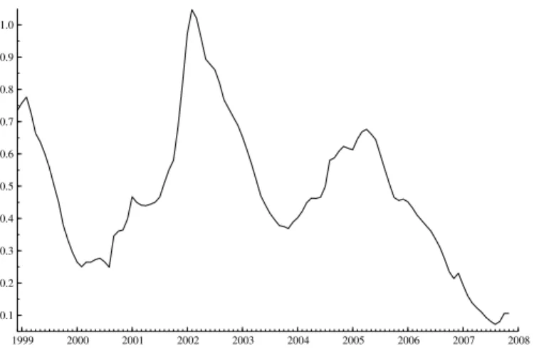
The estimates shown in figures 2.4, 2.5 and 2.6 are the long run estimates for the pass-through.
2000 2001 2002 2003 2004 2005 2006 2007 2008 0.00
0.25 0.50
2000 2001 2002 2003 2004 2005 2006 2007 2008
0.0 0.5
2000 2001 2002 2003 2004 2005 2006 2007 2008
0.5 0.6
Figure 2.2: IPA-OGPA smoothed coefficient of Δ log𝑒𝑡, Δ log𝑒𝑡−1 and Δ log𝑦𝑡−1.
over time. Although there are some periods in which it is not verified (i.e. from 2002 to 2003 and
from 2005 to 2006), its value keeps declining until where we see slightly increase 2008.
The high persistence produces high variations in the long run pass-through. For example, it
reaches values as high as 0.90 during the crisis period of 1999 and 2002 for all studied series. It
highlights the importance of the autoregressive term in the measurement equation for the long run.
The agricultural prices have had a step decline since 1999. Since the two peaks of 1999 and
2002, the long run pass-through has declined and converged to almost 0.20. One of the possible
explanations to this is a increase in the competition.
Industrial prices have a similar behavior, with more intense decline. After reaching values
around 1 in 2002, the exchange rate pass-through estimated values were around 0.1, 10% of the
value in the crisis period. It is important to notice that there was a peak in the decreasing trend
CHAPTER 2. PASS-THROUGH ESTIMATION IN BRAZIL 27
2000 2005
0.00 0.05 0.10 0.15 0.20
2000 2005
−0.2 0.0 0.2
2000 2005
0.55 0.60 0.65
2000 2005
0.00 0.05 0.10 0.15
Figure 2.3: IPA-OGPI smoothed coefficient of Δ log𝑒𝑡, Δ log𝑒𝑡−1(top), Δ log𝑦𝑡−1 and Δ log𝑦𝑡−6
(bottom).
the same time, world demand was growing sharply. This led to an increase in demand of industrial
goods because of a lack of competition. Therefore, cost movements and exchange rate changes
were more easily passed through to prices, including exchange rate changes. That is a possible
reason why the pass-through increased in this period. The central bank was forced to implement
a strong restrictive monetary policy that caused a reversion in inflation expectations and reduced
the exchange rate pass-through.
An important fact is the increase in pass-through in 2003 before the Brazilian elections. The
fear of macroeconomic policy changes caused a decrease in foreign investments. The expectation
was that the exchange rate would be devalued for a long time, consequently, agents anticipated
this expected devaluation and changed their prices. However, they realized that economic policies
2000 2001 2002 2003 2004 2005 2006 2007 2008 0.1
0.2 0.3 0.4 0.5 0.6 0.7 0.8
Figure 2.4: IPA-OG long run pass-through.
2000 2001 2002 2003 2004 2005 2006 2007 2008
0.2 0.3 0.4 0.5 0.6 0.7 0.8
CHAPTER 2. PASS-THROUGH ESTIMATION IN BRAZIL 29
1999 2000 2001 2002 2003 2004 2005 2006 2007 2008
0.1 0.2 0.3 0.4 0.5 0.6 0.7 0.8 0.9 1.0
Figure 2.6: IPA-OGPI long run pass-through.
through this valuation of domestic currency.
These results strongly reinforce the belief that the pass-through is declining in Brazil for
whole-sale prices. It is important to note that 1999 and 2002 were periods of much domestic uncertainty.
In January 1999, Brazil shifted from fixed to a flexible exchange rate regime and suffered a strong
crisis of credibility. According to the Calvo and Reinhart (2000) both lack of credibility and
volatility of exchange rate are linked to a high exchange rate pass-through.
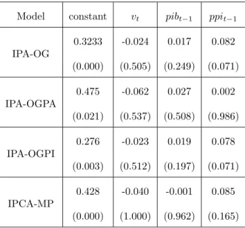
We tested whether the explanatory variables are significant in the model and we found that none
of the coefficients in the measurement equation were significant at the usual levels of significance.
Likelihood tests were conducted for the constant coefficients in the model. The results in Table
Table 2.4: Estimates of the IPA-OG, IPA-OGPA and IPA-OGPI series (p-values between
paren-thesis).
Model constant 𝑣𝑡 𝑝𝑖𝑏𝑡−1 𝑝𝑝𝑖𝑡−1
IPA-OG
0.3233 -0.024 0.017 0.082
(0.000) (0.505) (0.249) (0.071)
IPA-OGPA
0.475 -0.062 0.027 0.002
(0.021) (0.537) (0.508) (0.986)
IPA-OGPI
0.276 -0.023 0.019 0.078
(0.003) (0.512) (0.197) (0.071)
IPCA-MP
0.428 -0.040 -0.001 0.085
(0.000) (1.000) (0.962) (0.165)
at the usual significance levels3.
2.3.2
Determinants
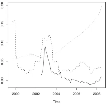
Some of the changes in the Brazilian economy appear to have exacerbated fluctuations in exchange
rates. The liberalization of capital flows in the last two decades and the increase in the scale of
cross-border financial transactions have increased exchange rate movements. Currency crises in
emerging market economies are unique examples of high exchange rate volatility. In Brazil, these
large movements in exchange rate may be associated with greater pass-through to prices as seen
in Figure 2.7.
Given the results presented in the previous section, we reformulate the model. Since the
3
CHAPTER 2. PASS-THROUGH ESTIMATION IN BRAZIL 31
2000 2002 2004 2006 2008
0.00
0.05
0.10
0.15
0.20
Time
Figure 2.7: Tested determinants of pass-through: Monetary policy, (solid line), variance of
ex-change rate (dashed line) and international trade (dotted line).
coefficients of the contemporaneous effect of the exchange rate on the wholesale price indexes are
mostly constant, we decide to introduce them with constant coefficients. The same was done to
the persistence coefficients. In addition, all variables statistically null in the former model were
excluded from the actual one. The only exception was the error term to control for endogeneity
of the contemporaneous log difference of exchange rate pass-through. Futhermore, we tried to test
the importance of some determinants of exchange rate pass-through. For this purpose, we made
changes in state equation and we introduced some explanatory variables in the state equation. As
Δ log 𝑝𝑡=𝛽1𝑡Δ log 𝑒𝑡−1+𝜓0+𝜓1Δ log 𝑒0+𝜓2Δ log𝑝𝑡−1+𝜀𝑡, 𝜀𝑡∼𝑁 𝐼𝐷(0, 𝜎2) (2.8)
𝛽𝑡+1=𝛽𝑡+𝛾𝑑𝑡+𝜂𝑡, 𝜂𝑡∼𝑁 𝐼𝐷(0, 𝑄). (2.9)
The former equation linearly relates the observed monthly log-variation of price to the log-variation
of exchange rate from time𝑡to time time𝑡−1 and to its own value at time𝑡−1. The coefficient
of Δ𝑙𝑜𝑔 𝑒𝑡−1 in equation (2.8) is the state coordinate and its dynamics are given in equation (2.9).
This equation now has the explanatory variable (or “determinant”),𝑑𝑡, with coefficient 𝛾and an
error term with variance𝑄.
Guided by the literature presented in the previous sections, we tested four explanatory variables
for the latent exchange rate pass-through coefficients: the difference between the exchange rate
variance of daily log returns from time𝑡 to time 𝑡−1, 𝑑𝑣𝑑𝑛𝑒𝑟𝑡; the variation of the ratio of the
inflation expectation and the inflation target set by the central bank from time𝑡 to time 𝑡−1,
𝑑𝑝𝑚𝑡; the log difference of the trade flow (given by the sum of exports and imports) divided by
the real GDP from time𝑡to time𝑡−1,𝑑𝑙𝑓 𝑙𝑜𝑤𝑡; and the log difference of the Brazilian IPCA (a
consumer price index computed by the Brazilian Census Bureau, IBGE) from time𝑡to time𝑡−1. We also included one lag for each variable because all these variables are likely to be endogenous.
The coefficient gamma represents the effect of each “determinant” over the dynamic of exchange
rate pass-through.
The monetary policy measure is the change in inflation expectation over the inflation target.
In an inflation targeting regime, the central bank uses one monetary policy rule to accommodate
inflation expectations close to the target set before. In an attempt to identify the success of the
CHAPTER 2. PASS-THROUGH ESTIMATION IN BRAZIL 33
average of the difference of inflation expectations of 12 months ahead over the inflation target. To
control for the monetary policy’s forward looking behavior, we set a moving weight, as follows
𝑝𝑚𝑡= (1/12)(𝐸𝑡(𝜋𝑡+12)−¯𝜋𝑡+12) + (1−𝑗/12)(𝐸𝑡+1(𝑡+ 13)−𝜋𝑡+13), (2.10)
for𝑗= 1, . . . ,12.
Mishkin (2008) stated that the correlation between inflation and the rate of nominal exchange
rate depreciation can indeed be high in an unstable monetary environment in which nominal shocks
fuel both high inflation and exchange rate depreciation. Furthermore, the evidence suggests that
even countries where inflation and exchange rate depreciation appear to be fairly closely linked
over time, have experienced a sizable decline in pass-through following the adoption of improved
monetary policies. To test if the credibility of the Brazilian Central Bank has been decreasing the
exchange rate pass-through, we created a monetary policy variable as the inflation expectation (by
Boletim FOCUS) over the inflation target. The credibility and the efficiency of the monetary policy
tend to hinder the ability of price makers to adjust their prices. In an stable inflation environment,
the agents are less likely to adjust their prices.
Taylor (2000) argues that the exchange rate pass-through has a positive relation to the
per-sistence of costs changes. If the volatility of changes in exchange rates is associated with its
persistence, smaller volatility periods will be followed by a smaller degree of pass-through. The
volatility in exchange rate can represent uncertainty in the economy, where large exchange rate
movements could more be easily passed through to prices.
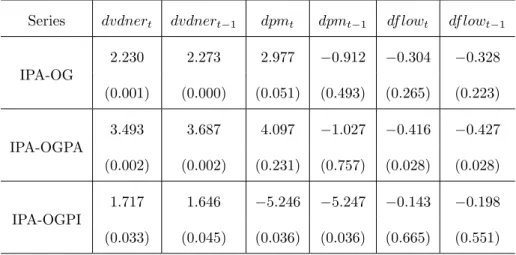
Our results show a statistical significant association between exchange rate volatility and
pass-through. In periods with high uncertainty, large variations in exchange rate are positively correlated
Table 2.5: Estimated parameters and corresponding p-values (in parenthesis).
Series 𝑑𝑣𝑑𝑛𝑒𝑟𝑡 𝑑𝑣𝑑𝑛𝑒𝑟𝑡−1 𝑑𝑝𝑚𝑡 𝑑𝑝𝑚𝑡−1 𝑑𝑓 𝑙𝑜𝑤𝑡 𝑑𝑓 𝑙𝑜𝑤𝑡−1
IPA-OG
2.230 2.273 2.977 −0.912 −0.304 −0.328 (0.001) (0.000) (0.051) (0.493) (0.265) (0.223)
IPA-OGPA
3.493 3.687 4.097 −1.027 −0.416 −0.427 (0.002) (0.002) (0.231) (0.757) (0.028) (0.028)
IPA-OGPI
1.717 1.646 −5.246 −5.247 −0.143 −0.198 (0.033) (0.045) (0.036) (0.036) (0.665) (0.551)
Table 2.6: Estimated parameters and corresponding p-values (in parenthesis).
Series 𝑑𝑙𝑛𝑡𝑟𝑎𝑑𝑒𝑓 𝑙𝑜𝑤/𝐺𝐷𝑃𝑡 𝑑𝑙𝑛𝑡𝑟𝑎𝑑𝑒𝑓 𝑙𝑜𝑤/𝐺𝐷𝑃𝑡−1 𝑑𝑙𝑛𝐼𝑃 𝐶𝐴𝑡 𝑑𝑙𝑛𝐼𝑃 𝐶𝐴𝑡−1
IPA-OG
−0.178 −0.179 −0.005 −0.005 (0.551) (0.569) (0.484) (0.423)
IPA-OGPA
−0.535 −0.565 −0.007 −0.006 (0.033) (0.026) (0.322) (0.291)
IPA-OGPI
−0.224 −0.136 −0.001 −0.002 (0.447) (0.666) (0.858) (0.817)
pass-through dynamics for all price indexes, more strongly agricultural prices. The trade openness
variable is only significant for exchange rate pass-through to agricultural prices. If an economy
is more open to foreign goods, it will face more competition and market power of producers will
decrease. For the whole IPA and for industrial products, the increase in imports share is less
pronounced and the effect over pass-through decline is not statistically significant. In the case of
CHAPTER 2. PASS-THROUGH ESTIMATION IN BRAZIL 35
the sector and reduced the propensity to pass-through cost changes to prices.
For the monetary policy variable, we found mixed results. For agricultural prices, the monetary
policy did not explain the pass-through. However, the exchange rate pass-through to industrial
prices was negatively associated with the monetary policy, where a large misalignment between
inflation expectations and the target is related to a smaller pass-through. We found that credibility
and a smaller deviation of expectation over the inflation target decrease the incentives to readjust
prices for the IPA only.
The variable𝑑𝑙𝑛𝐼𝑃 𝐶𝐴was introduced as an attempt to capture the inflationary environment.
With this variable we did not obtain evidence that the inflation environment affects the exchange
rate pass-through, as shown by table 2.6.
2.4
Conclusions
In this paper we estimated the evolution of the exchange rate pass-through for some wholesale
indexes prices in Brazil with a Gaussian state space model.
Using our formulation we were able to investigate some important aspects as endogeneity
be-tween exchange rate pass-through and the indexes prices, aggregation effects and persistence
vari-ation over time. We were also able to investigate the significance of some possible “determinants”
of exchange rate pass-through.
The estimates shown suggest that the the short run and long run exchange rate pass-through
are declining over time. Around 2002, the presidential election year President Lula ran for office,
the short run pass-through had risen to approximates one. Since then, the short run pass-through
variable are constant over time, indicating that the persistence of inflation is not varying. This
implies that if the long run pass-through changes over time, it is be due to the variation of the
short run pass-through.
We did not find strong evidence that there are important endogeneity from Brazilian wholesale
price indexes on exchange rate.
The data for the wholesales indexes does not support the null and the full exchange rate
pass-through hypotheses. This reinforces the belief that there exists a positive, although incomplete,
exchange rate pass-through in Brazil. For illustration propose, we estimated our model to a
Brazilian price index for monitored prices. In this case the estimates confirmed our previous belief
that there is no exchange rate pass-through for monitored prices.
Finally, we motivated and tested the importance of set exchange rate pass-through determinants
suggested by the literature on exchange rate pass-through. We obtained strong evidence that the
variance of exchange rate causes a greater pass-through to prices. We also obtained evidence that
some variables are able to explain the pass-through of some index prices but not of others. For
example, we found evidence that adjusting monetary policy led to a reduction in the pass-through
to industrial prices but not to agricultural prices. On the other hand, an increase in trade flow
results in a decrease the pass-through to agricultural prices but not to industrial prices. We had
Part II
Coincident and Leading Indexes of
Economic Activity
A State Space Model for Indices
of Economic Activity
3.1
Introduction
Traditionally, business-cycle research has focused on sophisticated econometric models aiming to
capture the main features of either GDP or of the four coincident variables that the NBER is
said to follow (employment, industrial production, income and sales) to estimate coincident and
leading indices of economic activity, establish business-cycle turning points, as well as to estimate
their respective probability of occurrence; see Stock and Watson (1988a, 1988b, 1989, 1991, 1993a),
Hamilton (1989), Kim and Nelson (1998), Harding and Pagan (2003), Hamilton (2003), and
Chau-vet and Piger (2008),inter-alia. Arguably, these models mis a key variable that should be included
in them – the NBER decisions on U.S. turning points as determined by its business-cycle dating
CHAPTER 3. A STATE SPACE MODEL FOR INDICES OF ECONOMIC ACTIVITY 39
committee. Although this information is usually available with a considerable lag, there is no
reason not to include it ex-post on econometric models. This point was forcefully made in Issler
and Vahid (2006).
There has been a recent trend of incorporating NBER dating-committee decisions into different
business cycle econometric models. Although some of these contributions are independent, they all
recognize that one should not discard the informational content of these decisions when constructing
econometric models; see Birchenhall et al. (1999), Dueker (2005), Issler and Vahid, and Chauvet
and Hamilton (2006). A key aspect of the NBER dating committee is that there are some changes in
its members through time. Additionally, shocks hitting the economy affect GDP and key economic
variables that the NBER is said to follow in a different manner, either happens because these
shocks vary across time (i.e., supply shocks in one recession and demand shocks in another) or
because some of these relationships are indeed not stable. Thus, in building econometric models
using the NBER-committee decisions we should consider the possibility of time-varying weights in
econometric relationships.
Our first original contribution is to propose a state-space model with time-variable weights
using the decisions to construct coincident and leading indices of economic activity for the U.S.
economy. Our model is a probit regression of NBER decisions on the coincident series, where
instrumental-variable techniques are needed to consistently estimate time-varying weights of this
index. In estimation, we apply the extended iterated Kalman filter and use the Rivers and Voung
(1988) procedure to correct for simultaneity. Also, we account for the fact that NBER decisions
on whether there is or not a recession at time𝑡 is made well into the future, i.e., in time𝑡+ℎ,
ℎ >0.