STOCHASTIC PROGRAMS BASED ON EXTENDED POLYHEDRAL RISK MEASURES
VINCENT GUIGUES
Abstract. We consider risk-averse convex stochastic programs expressed in terms of extended polyhedral
risk measures. We derive computable confidence intervals on the optimal value of such stochastic programs using the Robust Stochastic Approximation and the Stochastic Mirror Descent (SMD) algorithms. When the objective functions are uniformly convex, we also propose a multistep extension of the Stochastic Mirror Descent algorithm and obtain confidence intervals on both the optimal values and optimal solutions. Nu-merical simulations show that our confidence intervals are much less conservative and are quicker to compute than previously obtained confidence intervals for SMD and that the multistep Stochastic Mirror Descent algorithm can obtain agood approximate solution much quicker than its nonmultistep counterpart. Our confidence intervals are also more reliable than asymptotic confidence intervals when the sample size is not much larger than the problem size.
AMS subject classifications: 90C15, 90C90.
1. Introduction
Consider the convex stochastic optimization problem (1.1)
min f(x) :=R[g(x, ξ)], x∈X,
whereξ∈Lp(Ω,F,P;Rs) is a random vector with support Ξ and with
• g:E×Rs→Ra Borel function which is convex inxfor everyξandP-summable inξfor everyx; • X a closed and bounded convex set in a Euclidean spaceE;
• Ran extended polyhedral risk measure [11]; and • f :X →Ra convex Lipschitz continuous function.
Given a sampleξ1, . . . , ξN from the distribution ofξ, our goal is to obtainonline nonasymptotic computable
confidence intervals for the optimal value of (1.1) using as estimators of the optimal valuevariants of the
Stochastic Mirror Descent (SMD) algorithm. By computable confidence interval, we mean a confidence
interval that does not depend on unknown quantities. For instance, the confidence intervals from [19] and [12] are obtained using SMD and a variant of SMD but are not computable since they require the evaluation of the objective functionf at the approximate solution and typically for problems of form (1.1) this evaluation cannot be performed exactly. The terminology online, taken from [17], refers to the fact that the confidence intervals are computed in terms of the sampleξN = (ξ
1, . . . , ξN) used to solve problem (1.1), whereas offline
confidence intervals use an additional sample ξN˜ = (ξ
N+1, . . . , ξN+ ˜N) independent on ξN. Contrary to
asymptotic confidence intervals that are valid as the sample size tends to infinity, nonasymptotic confidence bounds use probability inequalities that are valid for all sample sizes, but they can be more conservative for this reason.
Before deriving a confidence interval on the optimal value of stochastic program (1.1), we need to define estimators of this optimal value. A natural estimator for this optimal value is the empirical estimator which is obtained replacing the risk measure in the objective function by its empirical estimation.1 In the case of risk-neutral convex problems (whenR=Eis the expectation), asymptotic and consistency properties of this estimator have been studied extensively. The asymptotic distribution of the empirical estimator is obtained
Key words and phrases. Stochastic Optimization, Risk measures, Multistep Stochastic Mirror Descent, Robust Stochastic Approximation.
1Note, however, that in this case a solution method still needs to be specified to solve the corresponding approximate
problem.
using the Delta method (see [28], [34]) and the Functional Central Limit Theorem. This distribution and the consistency of the estimator were derived in [6], [31], [32] [14], [21], [2], [3], [4]. In [18] the confidence intervals are built using a multiple replication procedure while a single replication is used in [2]. The paper [5] deals more specifically with the computation of asymptotic confidence intervals for the optimal value of risk-neutral multistage stochastic programs. These results were extended to some stochastic programs with integer recourse in [16] and [8].
Less papers have focused on the determination of nonasymptotic confidence intervals on the optimal value of a stochastic convex program. This problem was however studied in [22] for risk-neutral convex problems using Talagrand inequality ([35], [36]). Similar results, using large-deviation type results are obtained in [33] and in [15], [16] for integer models. Instead of using the empirical estimator, the optimal value of (1.1) can be estimated using algorithms for stochastic convex optimization such as the Stochastic Approximation (SA) [26], the Robust Stochastic Approximation (RSA) [24], [25], or the Stochastic Mirror Descent (SMD) algorithm [19]. This approach is used in [19] and [17] where nonasymptotic confidence intervals on the optimal value of a stochastic convex program are derived.
The SMD algorithm applied to stochastic programs minimizing the Conditional Value-at-Risk (CVaR, introduced in [27]) of a cost function was studied in [17]. However, we are not aware of papers deriving confidence intervals for the optimal values of stochastic risk-averse convex programs expressed in terms of large classes of risk measures, namely law invariant coherent or extended polyhedral risk measures (EPRM).
In this context, the contributions of this paper are the following:
(A) the description and convergence analysis of Stochastic Mirror Descent is based on three important assumptions: (i) convexity of the objective function, (ii) a stochastic oracle provides stochastic subgradients, and (iii) bounds on some exponential moments are available. We extend the SMD algorithm to solve risk-averse stochastic programs that minimize an EPRM of the cost. We provide conditions on these risk measures such that the aforementioned conditions (i), (ii), and (iii) hold and give a formula for stochastic subgradients of the objective function in this situation. Examples of EPRM satisfying these conditions are the expectation, the CVaR, some spectral risk measures, the optimized certainty equivalent, the expected utility with piecewise affine utility function, and any linear combination of these. We also observe that such stochastic programs can be reformulated as risk-neutral stochastic programs with additional variables and constraints, making the SMD for risk-neutral problems directly applicable to these reformulations.
(B) We provide conditions ensuring that assumptions (i), (ii), and (iii) are satisfied for two-stage sto-chastic risk-neutral programs and give again formulas for stosto-chastic subgradients of the objective function in this case.
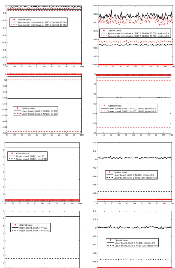
(C) We define a new computable nonasymptotic online confidence interval on the optimal value of a risk-neutral stochastic convex program using SMD. Numerical simulations show that this confidence interval is much less conservative than the online confidence interval from [17] and is more quickly computed.
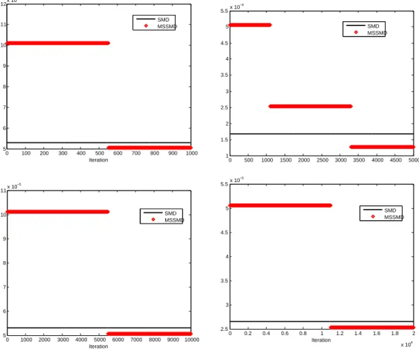
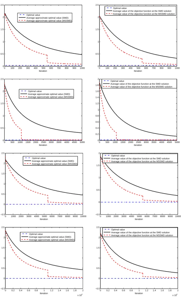
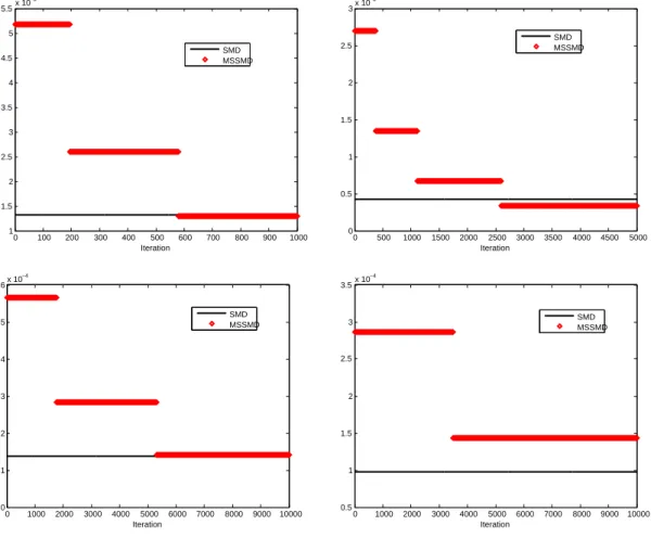
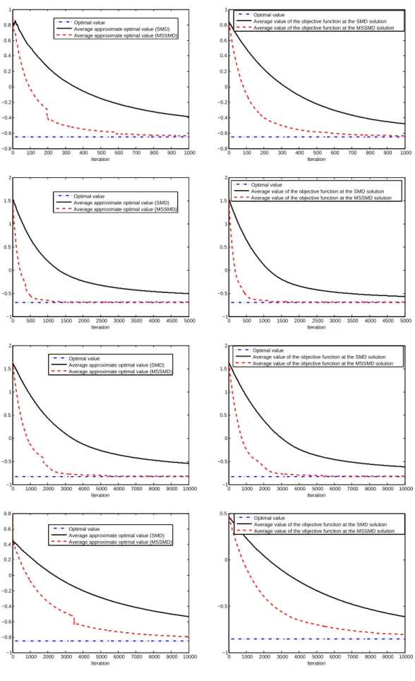
(D) We apply the ideas of the multistepmethod of dual averagingdescribed in [12] to propose a multistep Stochastic Mirror Descent algorithm. We also analyse the convergence of this variant of SMD and provide computable confidence intervals on the optimal value using this algorithm (contrary to [12] where for the stochasticmethod of dual averagingthe confidence intervals were not computable). We present the results of numerical simulations showing the interest of the multistep variant of SMD on two stochastic (uniformly) convex optimization problems.
(E) We study the convergence of SMD when the objective function is uniformly convex.
produces an approximate optimal value gN for (1.1) and a confidence interval for that optimal value. In
the particular case when the objective function f is uniformly convex, we additionally provide confidence intervals for the optimal solution of (1.1). Applying the techniques discussed in [12] to the SMD algorithm, multistep versions of the Stochastic Mirror Descent algorithm are proposed and studied in Section 4 in the case when f is uniformly convex. Confidence intervals for the optimal value of (1.1) obtained using these multistep algorithms are also given. In Section 5 numerical simulations illustrate our results: we show the interest of the multistep variant of SMD over its traditional, nonmultistep, implementation. Finally, in Section 6, we comment on future directions of research.
We use the following notation. For a vector x ∈ Rn, x+ is the vector with i-th component given by
x+(i) = max(x(i),0). We denote byf′(x) one of the subgradient(s) of convex functionf atx. For a norm
k · kof a Euclidean spaceEassociated to a scalar producth·,·i, the normk · k∗conjugate tok · kis given by
kyk∗= max x:kxk≤1hx, yi.
We denote theℓpnorm of a vectorxinRnbykxkp. The ball of centerx0and radiusRis denoted byB(x0, R). By ΠY, we denote the metric projection operator onto the setY, i.e., ΠY(x) = arg miny∈Y ky−xk2. For a
nonempty setX ⊆Rn, the polar coneX∗ is defined byX∗={x∗ :hx, x∗i ≤0, ∀x∈X}, whereh·,·iis the standard scalar product onRn. Byξt= (ξ
1, . . . , ξt), we denote the history of the process up to timet and
byFt the sigma-algebra generated by ξt. We will denote the Hessian matrix of f at xby f′′(x). Finally,
unless stated otherwise, all relations between random variables are supposed to hold almost surely.
2. Class of problems considered and assumptions
Consider problem (1.1) withRan EPRM:
Definition 2.1. [11] Let (Ω,F,P) be a probability space and let K(z) = (K1(z), . . ., Kn2,2(z))⊤ for given
functions2 K
1, . . . , Kn2,2 : R → R. A risk measure R on Lp(Ω,F,P) with p ∈ [2,∞) is called extended polyhedral if there exist matrices A1, A2, B2,0, B2,1, and vectors a1, a2, c1, c2 such that for every random
variableZ∈Lp(Ω,F,P)
(2.2) R(Z) =
infc⊤
1y1+E[c⊤2y2]
y1∈Rk1, y2∈Lp(Ω,F,P;Rk2), A1y1≤a1, A2y2≤a2a.s.,
B2,1y1+B2,0y2=K(Z)a.s. In what follows, we make the following assumption onK in (2.2):
(A0’) The functionK(z) is affine: K(z) =zk2+ ˜k2 for some vectorsk2,˜k2. Representation (2.2) can alternatively be written
(2.3) R(Z) =
infy1 c
⊤
1y1+E[Q(y1, Z)]
A1y1≤a1, where the recourse functionQ(y1, z) is given by
(2.4) Q(y1, z) =
infy2 c
⊤ 2y2
A2y2≤a2
B2,0y2=zk2+ ˜k2−B2,1y1.
In other words,R(Z) is the optimal value of a two-stage stochastic program whereZ appears in the right-hand side of the second-stage problem. It follows that we can re-write (1.1) as
(2.5)
( inf
y1,x
c⊤ 1y1+E
h
Qy1, g(x, ξ) i
A1y1≤a1, x∈X,
2The number of componentsn
2,2ofKcould be denoted bynto alleviate notation. We chose to use, as in [11], the notation
n2,2where these one-period EPRM are seen as special cases of multiperiod (T-periods) EPRM for which additional parameters
with Q(·,·) given by (2.4). This problem is of the form (1.1) with R the expectation and with x, g(x, ξ), and X respectively replaced by ˜x = (y1, x), ˜g(˜x, ξ) = c⊤1y1+Q
y1, g(x, ξ)
, and ˜X ={x˜ = (y1, x) : x∈
X, A1y1≤a1}.
For this reason, in Sections 3 and 4, we focus on risk-neutral stochastic problems of the form (2.6)
min f(x) :=E[g(x, ξ)], x∈X.
However, our analysis is based on some assumptions on f, X, and ξ, to be described in the next section. When reformulating risk-averse problem (1.1) under the form (2.6), introducing additional variables and constraints, one has to make some assumptions on the problem structure and on the EPRM in such a way that this reformulation (2.6) of the problem satisfies our assumptions. This issue is addressed in Subsection 2.3.
2.1. Assumptions. For problem (2.6), in addition to the assumptions onf andX mentioned in the intro-duction, we make the following assumptions:
Assumption 1. All subgradients of the objective function are bounded onX: there exists 0≤L <+∞such thatkf′(x)k∗≤Lfor every x∈X.
Note that Assumption 1 holds iff is finite in a neighborhood ofX.
Stochastic Oracle. We assume that samples ofξcan be generated and the existence of astochastic ora-cle: att-th call to the oracle,x∈X being the query point, the oracle returnsg(x, ξt)∈Rand a measurable
selectionG(x, ξt) of a stochastic subgradientG(x, ξt)∈∂xg(x, ξt), whereξ1, ξ2, ...is an i.i.d sample ofξ. We treatg(x, ξ) as an estimate off(x) andG(x, ξ) as an estimate of a subgradient of f atx.
Assumption 2. Our estimates are unbiased:
∀x∈X :f(x) =Eξ[g(x, ξ)] and f′(x) :=Eξ[G(x, ξ)]∈∂f(x).
From now on, we set
(2.7) δ(x, ξ) =g(x, ξ)−f(x), ∆(x, ξ) =G(x, ξ)−f′(x),
so that
Eξ[δ(x, ξ)] = 0, Eξ[∆(x, ξ)] = 0.
In the sequel, we assume that the observation errors of our oracle satisfy some assumptions (introduced in [19]) additional to having zero means. Specifically, ourminimalassumption is the following:
Assumption 3. For someM1, M2∈(0,∞) and for allx∈X
(2.8)
(a) Ehδ2(x, ξ)i
≤ M2 1, (b) Ehk∆(x, ξ)k2
∗
i
≤ M2 2.
Under our minimal assumption, we will obtain an upper bound on the average error on the optimal value of (1.1). To obtain a confidence interval on this optimal value, we will need a stronger assumption:
Assumption 4. For someM1, M2∈(0,∞) and for allx∈X it holds that
(2.9)
(a) Ehexp{δ2(x, ξ)/M2 1}
i
≤ exp{1},
(b) Ehexp{k∆(x, ξ)k2
∗/M22} i
≤ exp{1}.
Note that condition (2.9) is indeed stronger than condition (2.8): if a random variableY satisfiesEhexp{Y}i≤
exp{1}then by Jensen inequality, using the concavity of the logarithmic function,E
h
Yi=E
h
lnexp{Y}i≤
For a given confidence level, a smaller confidence interval can be obtained under an even stronger assump-tion:
Assumption 5. For someM1, M2∈(0,∞) and for allx∈X it holds that
(2.10) (a) E
h
exp{δ2(x, ξ)/M2 1}
i
≤ exp{1},
(b) k∆(x, ξ)k∗ ≤ M2almost surely.
Observe that the validity of (2.10) for allx∈X and someM1, M2 implies the validity of (2.9) for allx∈X with the sameM1, M2.
The computation of the confidence intervals on the optimal value of (1.1) using the SMD and multistep SMD algorithms presented in Sections 3 and 4 requires the knowledge of constantsL, M1, andM2satisfying the assumptions above. For instance, the best (smallest) constants M1, M2 satisfying Assumption 4 are
M1= supx∈Xπ[δ(x,·)] andM2= supx∈Xπ[k∆(x,·)k∗] whereπis the Orlicz semi-norm given by π[g] = infM ≥0 : E{exp{g2(ξ)/M2}} ≤exp{1} .
For many problems of form (1.1) withR=Ethe expectation operator, upper bounds on these best constants can be computed analytically, see for instance [19], [17], [10]. Throughout the paper, we will use two (classes) of problems of form (1.1) for which we will detail the computation of the parameters necessary to obtain the confidence intervals on their optimal value given in Sections 3 and 4, in particular parameters L, M1, and
M2 introduced above:
(1) The first class of problems writes
(2.11)
(
minf(x) =E
h
α0ξ⊤x+α21
(ξ⊤x)2+λ 0kxk22
i
x∈X :={x∈Rn:Pin=1xi =a, xi≥b, i= 1, . . . , n},
where n≥3, α1, a > 0,b, λ0 ≥0, withb < a/n, and the support Ξ of ξ is a part of the unit box {ξ= [ξ1;...;ξn]∈Rn:kξk∞≤1}.3
Ifa= 1 andb = 0, takingk · k=k · k1, k · k∗ =k · k∞, straightforward computations (see [10])
show that Assumptions 1-5 are satisfied for this problem with L=|α0|+α1, M1 = 2|α0|+ 0.5α1, andM2= 2|α0|+α1.
Now ifa= 1 andb= 0, takingk · k=k · k2=k · k∗, andG(x, ξ) =α0ξ+α1(ξξ⊤+λ0I)x, we have for everyx∈X that
kG(x, ξ)−E[G(x, ξ)]k2 ≤ |α0|kξ−E[ξ]k2+α1k(ξξ⊤−V)xk2
≤ 2|α0|√n+α1√nkξξ⊤−Vk∞≤2|α0|√n+ 2α1√n, kE[G(x, ξ)]k2 ≤ α0kE[ξ]k2+α1√nkE[ξξ⊤] +λ0Ik∞
≤ α0√n+α1(1 +λ0)√n,
and Assumptions 1 and 4 hold with L = α0√n+α1(1 +λ0)√n, M1 = 2|α0|+ 0.5α1, and M2 = 2|α0|√n+ 2α1√n.
(2) The second class of problems amounts to minimizing a linear combination of the expectation and the CVaR of some random linear function:
(2.12)
minf(x) =α0E[ξ⊤x] +α1CV aRε(ξ⊤x)
Pn
i=1xi= 1, x≥0,
where α1, α0 ≥0, 0 < ε < 1, the support Ξ of ξ is a part of the unit box {ξ = [ξ1;...;ξn] ∈Rn :
kξk∞≤1}, and
CVaRε(ξ⊤x) = min x0∈R
x0+E
ε−1[ξ⊤x
−x0]+
is the Conditional Value-at-Risk of level 0 < ε < 1, see [27]. Observing that |ξ⊤x| ≤ 1 a.s., the above problem is of the form (1.1) with X = {x= [x0;x1;...;xn]∈ Rn+1 : |x0| ≤1, x1, ..., xn ≥
0, Pni=1xi = 1}and
g(x, ξ) =α0ξ⊤[x1;...;xn] +α1
x0+ 1
ǫ[ξ
⊤[x1;...;x
n]−x0]+
.
3Ifb=a/nthen there is only one feasible point given byx
We will also consider a perturbed version of this problem given by
(2.13)
minα0E[ξ⊤x] +α1 x0+E
ε−1[ξ⊤x−x0]++λ
0k[x0;x1;...;xn]k22 −1≤x0≤1,Pni=1xi= 1, xi≥0, i= 1, . . . , n,
for λ0 > 0. For problem (2.13), taking k · k = k · k2 = k · k∗, we compute (see [10]) L =
q
α2
1(1−1ε)2+n(α0+ α1
ε )2+ 2λ0,M1= 2(α0+ α1
ε ), andM2=
q
α1
ε
2
+ 4n α0+αε1 2
.
2.2. Two-stage stochastic convex programs. Consider the case when (1.1) is a two-stage risk-neutral stochastic convex program, i.e., R = E is the expectation, x is the first-stage decision variable, f(x) =
f1(x) +Eξ[Q(x, ξ)] whereQ(x, ξ) is the second-stage cost given by
(2.14) Q(x, ξ) =
miny f2(x, y, ξ)
y∈ S(x, ξ) ={y:g2(x, y, ξ)≤0, Ax+By=ξ}
for some function g2 taking values inRm and some random vectorξ∈Lp(Ω,F,P) with p≥2 and support
Ξ. We make the following assumptions:
(A0) X ⊂Rp′ is a nonempty, compact, and convex set;
(A1) f1 is convex, proper, lower semicontinuous, and is finite in a neighborhood ofX;
(A2) for every x∈X andy∈Rq the functionf2(x, y,·) is measurable and for everyξ∈Ξ, the function
f2(·,·, ξ) is differentiable, convex, and proper;
(A3) for everyξ∈Ξ, the functiong2(·,·, ξ) is convex and differentiable;
(A4) for every x∈X and for everyξ∈Ξ the setS(x, ξ) is compact and there existsyx,ξ∈ S(x, ξ) such
thatg2(x, yx,ξ, ξ)<0.
With the notation of Section 1, we have f(x) = E[g(x, ξ)] where g(x, ξ) = f1(x) +Q(x, ξ). Assumptions (A1), (A2), and (A3) imply the convexity off. Assumptions (A2) and (A4) imply that for everyξ∈Ξ, the second-stage costQ(x, ξ) is finite which implies the finiteness ofδ(x, ξ) for everyx∈X. Relations (2.8)(a), (2.9)(a), and (2.10)(a) in respectively Assumptions 3, 4, and 5 are thus satisfied. Assumptions (A2), (A3), and (A4) imply that for every ξ ∈ Ξ, the function x → Q(x, ξ) is subdifferentiable on X with bounded subgradients at any x ∈ X. For fixed x∈ X and ξ ∈Ξ, let y(x, ξ) be an optimal solution of (2.14) and consider the dual problem
(2.15) sup
(λ,µ)
θx,ξ(λ, µ)
for the dual function
θx,ξ(λ, µ) = inf
y f2(x, y, ξ) +λ
⊤(Ax+By
−ξ) +µ⊤g2(x, y, ξ).
Let (λ(x, ξ), µ(x, ξ)) be an optimal solution of (2.15) (for problem (2.14), λ(x, ξ) and µ(x, ξ) are optimal Lagrange multipliers for respectively the equality and inequality constraints). Then for any x ∈ X and
ξ∈Ξ, denoting byI(x, y, ξ) :={i∈ {1, . . . , m}:g2,i(x, y, ξ) = 0} the set of active inequality constraints at y for problem (2.14),
s(x, ξ) =∇xf2(x, y(x, ξ), ξ) +A⊤λ(x, ξ) +
X
i∈I(x,y(x,ξ),ξ)
µi(x, ξ)∇xg2,i(x, y(x, ξ), ξ)
belongs to the subdifferential∂xQ(x, ξ) and is bounded (see [9] for instance for a proof). As a result, for any x∈X, denoting by s1(x) an arbitrary element from∂f1(x), f′(x) :=E[G(x, ξ)] is a subgradient off atx
forG(x, ξ) =s1(x) +s(x, ξ) and recalling that (A1) holds,kG(x, ξ)k∗ is bounded for anyx∈X andξ∈Ξ.
It follows that Assumption 1 is satisfied as well as Relations (2.8)(b), (2.9)(b), and (2.10)(b) in respectively Assumptions 3, 4, and 5.
2.3. Risk-averse stochastic convex programs. Consider reformulation (2.5) of problem (1.1). To guar-antee the convexity of the objective function in this problem as well as Assumptions 1-5, we make the following assumptions onRandg:
(A1’) Complete recourse: Y1 :={y1 :A1y1≤a1}is nonempty and bounded and{B2,0y2:A2y2 ≤a2}=
(A2’) The feasible set
(2.16) D={λ= (λ1, λ2)∈Rn2,2×Rn2,1 : λ2≤0, B⊤2,0λ1+A⊤2λ2=c2}
of the dual of the second-stage problem (2.4) is nonempty. (A3’) The setDgiven by (2.16) is bounded.
(A4’) For the setDgiven by (2.16), we have thatD ⊆ {−k2}∗×Rn2,1.
(A5’) For everyξ∈Ξ, the functiong(·, ξ) is convex and lower semicontinuous onX and the subdifferential
∂xg(x, ξ) is bounded for every x∈X.
IfX is closed, bounded, and convex, (A1’) implies that ˜X is also closed, bounded and convex. Moreover, we can show that assumptions (A1’), (A2’), (A3’), (A4’), and (A5’) imply that the objective function in (2.5) is convex and has bounded subgradients:
Lemma 2.2. Consider the objective function f(˜x) = c⊤ 1y1+E
h
Qy1, g(x, ξ) i
of (2.5) in variable x˜ =
(y1, x). Assume that (A1’), (A2’), (A3’), (A4’), and (A5’) hold. Then
(i) Qy1, g(x,ξ˜)
is finite for everyξ˜and every x˜∈X˜;
(ii) for every ξ˜∈Ξ, the function x˜ →Q˜ξ˜(˜x) =Q
y1, g(x,ξ˜)
is convex and has bounded subgradients
onX˜;
(iii) f is convex and has bounded subgradients on X˜.
Proof. Since (A1’) holds, for everyy1∈Y1and everyz∈R, the feasible set of problem (2.4) which defines
Q(y, z) is nonempty. Due to (A2’), the feasible set of the dual of this problem is nonempty too. It follows that both the primal and the dual have the same finite optimal value (this shows item (i)) and by duality we can expressQ(y1, z) as the optimal value of the dual problem:
(2.17) Q(y1, z) = max
(λ1,λ2)∈D
λ⊤
1(zk2+ ˜k2−B2,1y1) +λ⊤2a2 withDgiven by (2.16). Next, observe thatQ(y1,·) is monotone:
(2.18) ∀y1∈Y1, ∀z1, z2∈R, z1≥z2⇒ Q(y1, z1)≥ Q(y1, z2). Indeed, ifz1≥z2, for every (λ1, λ2)∈ D, since (A4’) holds, we haveλ⊤1k2≥0 and
λ⊤
1(z1k2+ ˜k2−B2,1y1) +λ⊤2a2≥λ⊤1(z2k2+ ˜k2−B2,1y1) +λ⊤2a2
for every y1 ∈ Y1. Taking the maximum when (λ1, λ2) ∈ D in each side of the previous inequality gives Q(y1, z1)≥ Q(y1, z2). Now take ˜ξa realization ofξand ˜x= (y1, x),x˜0= (y01, x0)∈X˜. Using the convexity ofg(·,ξ˜), we have
g(x,ξ˜)≥g(x0,ξ˜) +G(x0,ξ˜)⊤(x−x0)
recalling thatG(x0, ξ) is a measurable selection of a stochastic subgradient ofg(·, ξ) atx0. Combining this inequality and (2.18) gives
˜
Qξ˜(˜x) =Q
y1, g(x,ξ˜)
≥ Qy1, g(x0,ξ˜) +G(x0,ξ˜)⊤(x−x0)
for everyy1∈Y1. Next, we have thatQ(y1, z) is convex and its subdifferential is given by
∂Q(y1, z) =
−B⊤ 2,1λ1
λ⊤ 1k2
: (λ1, λ2)∈ Dy1,z
whereDy1,z is the set of optimal solutions to the dual problem (2.17). Denoting by (λ1(y1, z), λ2(y1, z)) an optimal solution to (2.17), we then have
˜
Qξ˜(˜x) =Q
y1, g(x,ξ˜)
≥Q˜ξ˜(˜x0) +
−B⊤
2,1λ1(y01, g(x0,ξ˜))
λ1(y0
1, g(x0,ξ˜))⊤k2G(x0,ξ˜) ⊤
˜
x−x˜0
.
It follows that for every ˜ξ,Qξ˜(·) is convex and its subdifferential is given by
∂Q˜ξ˜(y01, x0) =
−B⊤ 2,1λ1
λ⊤
1k2G(x0,ξ˜)
: (λ1, λ2)∈ Dy0 1, g(x0,ξ˜)
SinceDy0
1, g(x0,ξ˜)is a subset of the bounded setDand since (A5’) holds, all subgradients of ˜Qξ˜(·) are bounded for every ˜ξ∈Ξ: we have proved (ii). Item (iii) follows from (ii) and the fact thatf is finite in a neighborhood
of ˜X.
It follows from Lemma 2.2-(iii) that Assumption 1 is satisfied. We also haveδ(˜x, ξ) =Qξ(˜x)−E[Qξ(˜x)],
which is finite for everyξ and ˜x∈ X˜ using Lemma 2.2-(i). It follows that relations (2.8)(a), (2.9)(a), and (2.10)(a) in respectively Assumptions 3, 4, and 5 are satisfied. Finally Lemma 2.2-(ii) shows that relations (2.8)(b), (2.9)(b), and (2.10)(b) in respectively Assumptions 3, 4, and 5 are also satisfied. This shows that we can use the developments of Sections 3.1, and 3.2 to solve the two-stage stochastic risk-averse convex optimization problem (1.1) and to obtain a confidence interval on its optimal value when Ris an EPRM and when assumptions (A0’), (A1’), (A2’), (A3’), (A4’), and (A5’) are satisfied.
Risk-averse stochastic programs expressed in terms of EPRMs share many properties with risk-neutral stochastic programs. Moreover, many popular risk measures can be written as EPRMs satisfying assump-tions (A0’), (A1’), (A2’), (A3’), and (A4’). Examples of such risk measures are the CVaR, some spectral risk measures, the optimized certainty equivalent and the expected utility with piecewise affine utility func-tion. We refer to Examples 2.16 and 2.17 in [11] for a discussion on these examples. Conditions ensuring that an EPRM is convex, coherent or consistent with second order stochastic dominance are given in [11]. Multiperiod versions of these risk measures are also defined in [11]. In this context, a convenient property of the corresponding risk-averse program is that we can write dynamic programming equations and solve it, in the case when the problem is convex, by decomposition using for instance Stochastic Dual Dynamic Programming (SDDP) [20]; see [11] for more details and examples of multiperiod EPRM. EPRM are an extension of the polyhedral risk measures introduced in [7] where the reader will find additional examples of (extended) polyhedral risk measures.
3. Quality of the solutions using RSA and SMD
We consider the RSA and SMD algorithms to solve problem (2.6).
3.1. Robust Stochastic Approximation Algorithm. In this section, we take k · k =k · k2 with dual norm kxk∗ =kxk2, meaning that (2.8), (2.9), and (2.10) hold with k · k∗ =k · k2. The Robust Stochastic
Approximation algorithm solves (2.6) as follows:
Algorithm 1: Robust Stochastic Approximation.
Initialization. Take x1 in X. Fix the number of iterations N−1 and positive deterministic stepsizes
γ1, . . . , γN.
Loop. Fort= 1, . . . , N−1, compute
(3.19) xt+1 = ΠX(xt−γtG(xt, ξt)).
Outputs:
(3.20) xN = 1
ΓN N
X
τ=1
γτxτ andgN =
1 ΓN
"N X
τ=1
γτg(xτ, ξτ)
#
with ΓN = N
X
τ=1
γτ.
Note that by convexity ofX, we havexN
∈X and afterN−1 iterations,xN is an approximate solution of
(2.6). The valuef(xN) is an approximation of the optimal value of (2.6), but it is not computable sincef is
not known. Denoting byx∗an optimal solution of (2.6), we introduce afterN−1 iterations the computable
approximation4
(3.21) gN = 1
ΓN
" N X
τ=1
γτg(xτ, ξτ)
#
4Note that the approximation depends on (x
1, . . . , xN, ξ1, . . . , ξN, γ1, . . . , γN) so we could write
gN(x
of the optimal value f(x∗) of (2.6) obtained using the points generated by the algorithm and information
from the stochastic oracle. Our goal is to obtain exponential bounds on large deviations of this estimate
gN off(x
∗) from f(x∗) itself, i.e., a confidence interval on the optimal value of (2.6) using the information
provided by the RSA algorithm along iterations. We need two technical lemmas. The first one gives an
O(1/√N) upper bound on the first absolute moment of the estimation error (the average distance ofgN to f(x∗)):
Lemma 3.1. Let Assumptions 1, 2, and 3 hold and assume that the number of iterationsN−1 of the RSA algorithm is fixed in advance with stepsizes given by
(3.22) γτ=γ=
DX
p 2(M2
2 +L2) √
N, τ = 1, . . . , N,
where
(3.23) DX= max
x∈X kx−x1k.
Let gN be the approximation off(x∗) given by (3.21). Then
(3.24) EhgN−f(x∗)
i
≤M1+DX p
2(M2 2 +L2) √
N .
Proof. Recalling (3.22), Γγτ
N =
1
N and letting
(3.25) fN = 1
N N
X
τ=1
f(xτ),
it is known (see [19], Section 2.2) that under our assumptions
(3.26) Ef(xN)
−f(x∗)≤EfN
−f(x∗)≤DX p
2(M2 2 +L2) √
N .
Since the main steps of the proof of (3.26) will be useful for our further developments, we rewrite them here. SettingAτ= 12kxτ−x∗k22, we can show (see Section 2.1 in [19] for instance) that
(3.27)
N
X
τ=1
γτhG(xτ, ξτ), xτ−x∗i ≤A1+ 1 2
N
X
τ=1
γτ2kG(xτ, ξτ)k2∗.
To save notation, let us set
(3.28) δτ =g(xτ, ξτ)−f(xτ),∆τ= ∆(xτ, ξτ), and Gτ =G(xτ, ξτ) =f′(xτ) + ∆τ.
Inequality (3.27) can be rewritten
(3.29)
N
X
τ=1
γτhf′(xτ), xτ−x∗i ≤ D
2
X
2 + 1 2
N
X
τ=1
γ2τkGτk2∗+ N
X
τ=1
γτh∆τ, x∗−xτi.
Taking into account that by convexity off we havef(xτ)−f(x∗)≤ hf′(xτ), xτ−x∗i, we get
(3.30)
f(xN)
−f(x∗) ≤ fN
−f(x∗) = 1 ΓN
N
X
τ=1
γτ
f(xτ)−f(x∗)
≤ Γ1
N
"
D2
X
2 + 1 2
N
X
τ=1
γτ2kGτk2∗+ N
X
τ=1
γτh∆τ, x∗−xτi
#
where the first inequality is due to the origin ofxN and to the convexity off.
Next, note that under Assumptions 1, 2, and 3, (3.31) EhkGτk2∗
i
=Ehkf′(xτ) + ∆τk2∗
i
≤2Ehkf′(xτ)k2∗+k∆τk2∗
i
≤2hM22+L2 i
Passing to expectations in (3.30), and taking into account that the conditional, ξτ−1:= (ξ
1, ..., ξτ−1) being
fixed, expectation of ∆τ is zero, whilexτ by construction is a deterministic function of ξτ−1, we get
Ehf(xN)−f(x∗)
i
≤ EhfN −f(x∗)
i ≤ D2 X+ N X τ=1 γ2 τE kGτk2∗
2ΓN
≤ Γ1
N
hD2
X
2 + (M 2 2+L2)
N
X
τ=1
γτ2
i
.
(3.32)
Using stepsizes (3.22), we have ΓN = DX √
N
√ 2(M2
2+L2)
. Plugging this value of ΓN into (3.32), we obtain the
announced inequality (3.26). We now show that
(3.33) EhgN −fN
i
≤ √M1
N.
First, note that
(3.34) gN−fN = 1
N N
X
τ=1
δτ.
By the same argument as above, the conditional,ξτ−1being fixed, expectation of δ
τ is 0, whence
Eh N X τ=1 δτ 2i = N X τ=1
Ehδτ2
i
≤N M12,
where the concluding inequality is due to (2.8)(a). We conclude that
EhgN−fN i
≤N1 v u u u tE N X τ=1 δτ
!2 ≤ 1
N
q
N M2 1 =
M1 √
N,
which is the announced inequality (3.33). Next, observe that by convexity of f, fN
≥ f(xN) and since xN
∈X, we havef(xN)
≥f(x∗), i.e.,fN −f(x∗)≥f(xN)−f(x∗)≥0, so that (3.26) and (3.33) imply E
h
|gN −f(x∗)|
i
≤ E
h
|gN−fN|+|fN −f(x∗)|
i =E
h
|gN −fN|i+E
h
fN−f(x∗)
i
≤ hM1+DX
q 2(M2
2+L2) i 1
√
N,
which achieves the proof of (3.24).
To proceed, we need the following lemma:
Lemma 3.2. Let ητ, τ = 1, . . . , N, be a sequence of real-valued random variables with ητ Fτ-measurable.
Let E|τ−1[·]be the conditional expectationE
·|ξτ−1. Assume that
(3.35) E|τ−1
h
ητ
i
= 0, E|τ−1 h
exp{η2τ}
i
≤exp{1}.
Then, for anyΘ>0,
(3.36) P
N
X
τ=1
ητ>Θ
√
N
!
≤exp{−Θ2/4}.
Proof. See the Appendix.
We are now in a position to provide a confidence interval for the optimal value of (2.6) using the RSA algorithm:
Proposition 3.3. Assume that the number of iterations N −1 of the RSA algorithm is fixed in advance
with stepsizes given by (3.22). LetgN be the approximation off(x
(i) if Assumptions 1, 2, 3, and 4 hold, for any Θ>0, we have
(3.37) P
gN −f(x∗)
>
K1(X) + ΘK2(X) √
N
≤4 exp{1}exp{−Θ}
where the constants K1(X) andK2(X) are given by
K1(X) =DX(M 2 2+ 2L2) p
2(M2 2+L2)
andK2(X) = DXM
2 2 p
2(M2 2 +L2)
+ 2DXM2+M1,
withDX given by (3.23).
(ii) If Assumptions 1, 2, 3, and 5 hold,(3.37)holds with the right-hand side replaced by(3+exp{1}) exp{−1
4Θ 2
}.
Proof. To prove (i), we shall first prove that for any Θ>0,
(3.38) P
fN
−f(x∗)> √2(MDX2 2+L2)N
h
M2
2+ 2L2+ Θ h
M2 2+ 2M2
p 2(M2
2+L2) ii
≤2 exp{1}exp{−Θ},
wherefNis given by (3.25). Using Assumption 1, we have
kGτk2∗=kf′(xτ)+∆τk2∗≤2(kf′(xτ)k∗2+k∆τk2∗)≤
2(L2+
k∆τk2∗). Combined with (3.30), this implies that
(3.39)
fN−f(x
∗) ≤ Γ1 N " D2 X 2 + N X τ=1
γτ2
L2+k∆τk2∗
# + 1 ΓN N X τ=1
γτh∆τ, x∗−xτi
≤ DX(M 2 2 + 2L2) p
2(M2 2 +L2)
√
N +
DXM22 p
2(M2 2 +L2)
√
NA+
2DXM2
N B
where
(3.40) A= 1
N M2 2
N
X
τ=1
k∆τk2∗ and B= 1
2DXM2
N
X
τ=1
h∆τ, x∗−xτi.
Setting ζτ =k∆τk2∗/M22 and invoking (2.9)(b), we get E h
exp{ζτ}
i
≤exp{1}for all τ≤N, whence, due to the convexity of the exponent,
E
h
exp{A}i=E
h exp{N1
N
X
τ=1
ζτ}
i ≤N1
N
X
τ=1
E
h
exp{ζτ}
i
≤exp{1}
as well. As a result,
(3.41) ∀Θ>0 :PA>Θ≤exp{−Θ}Ehexp{A}i≤exp{1−Θ}.
Now let us set ητ = 2DX1M2h∆τ, x∗−xτi, so that B =PNτ=1ητ. Denoting by E|τ−1 the conditional, ξτ−1 being fixed, expectation, we have
E|τ−1 h
ητ
i
= 0 and E|τ−1 h
exp{η2τ}
i
≤exp{1},
where the first relation is due to E|τ−1 h
∆τ
i
= 0 combined with the fact that x∗−xτ is a deterministic
function ofξτ−1, and the second relation is due to (2.9)(b) combined with the fact thatkx∗−xτk ≤2DX.
Using Lemma 3.2, we obtain for any Θ>0
(3.42) PB>Θ√N≤exp{−Θ2/4
}.
Combining (3.39), (3.41), and (3.42), we obtain for every Θ>0
(3.43) P f
N−f(x
∗)> DX(M
2 2+ 2L2) p
2(M2
2+L2)N +√Θ
N
"
DXM22 p
2(M2 2 +L2)
+ 2DXM2 #!
≤exp{1−Θ}+ exp{−Θ2/4
} ≤2 exp{1}exp{−Θ},
Next,
gN
−fN = M1
N
" N X
τ=1
χτ
#
, χτ = δτ M1
.
Observing thatχτ is a deterministic function ofξτ and that E|τ−1
h
χτ
i
= 0 and E|τ−1 h
exp{χ2τ}
i
≤exp{1},1≤τ ≤N
(we have used (2.9)(a)), we can use once again Lemma 3.2 to obtain for all Θ>0:
P
gN−fN >Θ√M1
N
≤exp{−Θ2/4} and
P
gN −fN <−Θ√M1
N
≤exp{−Θ2/4}.
Thus,
∀Θ>0 :P
gN−fN >Θ
M1 √
N
≤2 exp{−Θ2/4},
which, combined with (3.38) implies (3.37), i.e., item (i) of the lemma.
Finally, under Assumption 5, we havePA>1= 0, which combines with (3.41) to imply that ∀Θ>0 :P
A>Θ≤exp{1−Θ2},
meaning that the right-hand side in (3.38) can be replaced with exp{1−Θ2
}+ exp{−Θ2/4
}, which proves
item (ii).
Setting
(3.44) a(Θ, N) = Θ√M1
N andb(Θ, X, N) =
K1(X) + Θ(K2(X)−M1) √
N ,
we now combine the upper bound
(3.45) Up1(Θ1, N) = 1
N N
X
t=1
g(xt, ξt) +a(Θ1, N) =gN +a(Θ1, N),
from [17] with the lower bound
(3.46) Low1(Θ2,Θ3, N) =gN −b(Θ2, X, N)−a(Θ3, N),
from Proposition 3.3 to obtain a new confidence interval on the optimal valuef(x∗). Indeed, since f(x t)≥ f(x∗) almost surely, using Lemma 3.2 we get
P
Up1(Θ1, N)< f(x∗)
≤P
1
N N
X
t=1 h
g(xt, ξt)−f(xt)
i
<−Θ1√M1
N
≤e−Θ21/4.
Next, using the proof of Proposition 3.3, we can define sets S1, S2 ⊂Ω such that under Assumptions 1, 2, 3, and 5 we have P(S1)≥ 1−e1−Θ22 −e−Θ
2
2/4 (resp. P(S2) ≥1−e−Θ 2
3/4) and if ω ∈ S1 (resp. ω ∈ S2) then fN −b(Θ2, X, N) ≤ f(x∗) (resp. gN −fN ≤ a(Θ3, N)). Now observe that if ω ∈ S
1 ∩S2 then
f(x∗)≥Low1(Θ2,Θ3, N) which implies that
P(f(x∗)≥Low1(Θ2,Θ3, N))≥P(S1∩S2)≥1−e1−Θ 2 2−e−Θ
2
2/4−e−Θ 2 3/4. We deduce the following corollary of Proposition 3.3:
Corollary 3.4. Let Up1 and Low1 be the upper and lower bounds given by respectively (3.45) and (3.46).
Then if Assumptions 1, 2, 3, and 5 hold, for any Θ1,Θ2,Θ3>0, we have
(3.47) P(f(x∗)∈hLow1(Θ2,Θ3, N),Up1(Θ1, N)i)≥1−e−Θ21/4−e1−Θ 2 2−e−Θ
2
Remark 3.5. To equilibrate the risks, for the confidence intervalhLow1(Θ2,Θ3, N),Up1(Θ1, N) i
onf(x∗)to
have confidence level at least0<1−α <1, we can takeΘ1such thate−Θ2
1/4=α/2, i.e.,Θ1= 2pln(2/α),Θ3
such thate−Θ23/4=α/4, i.e.,Θ3= 2pln(4/α), and compute by dichotomyΘ2such thate1−Θ
2 2+e−Θ
2 2/4= α
4. Remark 3.6. If an additional sampleξ¯N˜ = ( ¯ξ1, . . . ,ξ¯N˜) independent onξN = (ξ1, . . . , ξN)is available, we
can use the upper boundUp2(Θ1, N,N˜) = N1˜
PN˜
t=1g(xN,ξ¯t) +a(Θ1,N˜) withxN given by (3.20), see [17].
3.2. Stochastic Mirror Descent algorithm. The algorithm to be described, introduced in [19], is given by aproximal setup, that is, by a norm k · konE and adistance-generating function ω(x) :X →R. This function should
• be convex and continuous onX, • admit a continuous onXo=
{x∈X:∂ω(x)6=∅}selectionω′(x) of subgradients, and
• be compatible withk · k, meaning that ω(·) is strongly convex, modulus µ(ω)>0, with respect to the normk · k:
(ω′(x)−ω′(y))⊤(x
−y)≥µ(ω)kx−yk2∀x, y∈Xo.
The proximal setup induces the following entities:
(1) the ω-center ofX given byxω= argminx∈Xω(x)∈Xo;
(2) the Bregman distanceor prox-function
(3.48) Vx(y) =ω(y)−ω(x)−(y−x)⊤ω′(x)≥ µ(ω)
2 kx−yk 2,
forx∈Xo,y
∈X (the concluding inequality is due to the strong convexity ofω); (3) the ω-radius ofX defined as
(3.49) Dω,X =
r 2hmax
x∈Xω(x)−xmin∈Xω(x)
i
.
Since (x−xω)⊤ω′(xω)≥0 for allx∈X, we have
(3.50)
∀x∈X: µ(2ω)kx−xωk2 ≤ Vxω(x) =ω(x)−ω(xω)−(x−xω)⊤ω′(xω)
| {z }
≥0 ≤ ω(x)−ω(xω)≤ 12D2ω,X,
and
(3.51) ∀x∈X:kx−xωk ≤ pDω,X
µ(ω). (4) The proximal mapping, defined by
(3.52) Proxx(ζ) = argminy∈X{ω(y) +y⊤(ζ−ω′(x))} [x∈Xo, ζ∈E],
takes its values inXo.
Taking x+ = Proxx(ζ), the optimality conditions for the optimization problem miny∈X{ω(y) + y⊤(ζ−ω′(x))} in whichx
+is the optimal solution read ∀y∈X : (y−x+)⊤(ω′(x+) +ζ
−ω′(x))≥0.
Rearranging the terms, simple arithmetics show that this condition can be written equivalently as (3.53) x+= Proxx(ζ)⇒ζ⊤(x+−y)≤Vx(y)−Vx+(y)−Vx(x+)∀y∈X.
Algorithm 2: Stochastic Mirror Descent.
Loop. Fort= 1, . . . , N−1, compute
(3.54) xt+1 = Proxxt(γtG(xt, ξt)).
Outputs:
(3.55) xN = 1
ΓN N
X
τ=1
γτxτ andgN = 1
ΓN
"N X
τ=1
γτg(xτ, ξτ)
#
with ΓN = N
X
τ=1
γτ.
The choice of ω depends on the feasibility set X. For the feasibility sets of problems (2.11) and (2.12), several distance-generating functions are of interest.
Example 3.7 (Distance-generating function for (2.11) and (2.12)). Forω(x) =ω1(x) = 1 2kxk
2
2 andk · k= k · k=k · k∗,Proxx(ζ) = ΠX(x−ζ)and the Stochastic Mirror Descent algorithm is the RSA algorithm given
by the recurrence (3.19).
Example 3.8 (Distance-generating function for problem (2.11) witha= 1 andb= 0). Let ωbe the entropy function
(3.56) ω(x) =ω2(x) =
n
X
i=1
xiln(xi)
used in[19]withk · k=k · k1andk · k∗=k · k∞. In this case, it is shown in[19] thatx+= Proxx(ζ)is given
by
x+(i) = x(i)e
−ζ(i) Pn
k=1x(k)e−ζ(k)
, i= 1, . . . , n,
and that we can take Dω2,X =
p
2 ln(n), µ(ω2) = 1, and x1 =xω2 = 1
n(1,1, . . . ,1)⊤. To avoid numerical
instability in the computation of x+= Proxx(ζ), we compute insteadz+ = ln(x+)from z= ln(x)using the
alternative representation
z+=w−ln(
n
X
i=1
ew(i))1where w=z−ζ−max
i [z−ζ]i.
Example 3.9(Distance-generating function for problem for problem (2.11) with 0< b < a/n.). Let k · k= k · k1,k · k∗=k · k∞, and as in [10],[13, Section 5.7], consider the distance-generating function
(3.57) ω(x) =ω3(x) = 1
pγ n
X
i=1
|xi|p with p= 1 + 1/ln(n) andγ=
1 exp(1) ln(n).
For everyx∈X, since p→ kxkp is nonincreasing andp >1, we getkxkp≤ kxk1=aandmaxx∈Xω3(x)≤
ap
pγ. Next, using H¨older’s inequality, for x ∈ X we have a =
Pn
i=1xi ≤ n1/qkxkp where 1p + 1q = 1.
We deduce that minx∈Xω3(x) ≥ a
p
pγn1/ln(n) and that Dω3,X ≤
q 2ap
pγ (1−n−1/ln(n)). We also observe that
DX ≤√2(a−nb)and that µ(ω3) = exp(1)na2−p: for x, y∈X we have
(ω′3(x)−ω3′(y))⊤(x−y) = 1
γ n
X
i=1
(yi−xi)(ϕ(yi)−ϕ(xi)) =
1
γ n
X
i=1
ϕ′(ci)(yi−xi)2
for some 0 < ci ≤ a where ϕ(x) = xp−1. Since ϕ′(ci) ≥ ϕ′(a) = (p−1)ap−2, we obtain that (ω3′(x)−
ω′
3(y))⊤(x−y)≥µ(ω3)ky−xk21 withµ(ω3) = exp(1)
na2−p. In this context, each iteration of the SMD algorithm
can be performed efficiently using Newton’s method: setting x+ = Proxx(ζ) and z = ζ−ω3′(x), x+ is the
solution of the optimization problemminy∈XPni=1(1/pγ)ypi+ziyi.Hence, there are Lagrange multiplersµ≥0
andν such thatµi(b−x+(i)) = 0, (1/γ)x+(i)p−1+zi−ν−µi = 0 fori= 1, . . . , n, and Pni=1x+(i) = a.
If x+(i) > b then µi = 0 and ν −zi = (1/γ)x+(i)p−1 > bp−1/γ, i.e., x+(i) = max((γ(ν −zi))
1
p−1, b).
If x+(i) = b then µi ≥ 0 can be written (1/γ)x+(i)p−1 = 1γbp−1 ≥ ν −zi. It follows that in all cases
x+(i) = max((γ(ν −zi))
1
p−1, b). Plugging this relation into Pn
i=1x+(i) = a, computing x+ amounts to
finding a root of the functionf(ν) =Pni=1max((γ(ν−zi))
1
In what follows, we provide confidence intervals for the optimal value of (2.6) on the basis of the points generated by the SMD algorithm, thus extending Proposition 3.3. We first need a technical lemma:
Lemma 3.10. Let e1, ..., eN be a sequence of vectors from E, γ1, ..., γN be nonnegative reals, and let u1, ..., uN ∈X be given by the recurrence
u1 = xω
uτ+1 = Proxuτ(γτeτ),1≤τ ≤N−1.
Then
(3.58) ∀y∈X :
N
X
τ=1
γτe⊤τ(uτ−y)≤
1 2D
2
ω,X+
1 2µ(ω)
N
X
τ=1
γτ2keτk2∗.
Proof. See the Appendix.
Applying Lemma 3.10 toeτ =G(xτ, ξτ) and in relation (3.58) specifying y as a minimizerx∗ of f over X, we get:
N
X
τ=1
γτG(xτ, ξτ)⊤(xτ−x∗)≤ 12Dω,X2 +
1 2µ(ω)
N
X
τ=1
γτ2kG(xτ, ξτ)k2∗.
Using notation (3.28) of the previous section, the above inequality can be rewritten
(3.59)
N
X
τ=1
γτ(xτ−x∗)⊤f′(xτ)≤ D2
ω,X
2 +
1 2µ(ω)
N
X
τ=1
γτ2kGτk2∗+ N
X
τ=1
γτ∆⊤τ(x∗−xτ).
We mentioned that whenω(x) = 1 2kxk2
2, the SMD algorithm is the RSA algorithm of the previous section. In that case, µ(ω) = 1, k · k = k · k2, k · k∗ = k · k2, and (3.59) is obtained from inequality (3.29) of the previous section for the RSA algorithm substitutingDX byDω,X (note that when choosingx1=xω for the
RSA algorithm, we haveDX ≤Dω,X so for the RSA algorithm (3.29) gives a tighter upper bound). We can
now extend the results of Lemma 3.1 and Proposition 3.3 to the SMD algorithm:
Lemma 3.11. Let Assumptions 1, 2, 3 and 4 hold and assume that the number of iterations N−1 of the SMD algorithm is fixed in advance with stepsizes given by
(3.60) γτ=γ=
Dω,X
p
µ(ω) p
2(M2 2 +L2)
√
N, τ = 1, . . . , N.
Consider the approximation gN = 1
N N
X
τ=1
g(xτ, ξτ)of f(x∗). Then
(3.61) EhgN −f(x∗)
i
≤
M1+
Dω,X
p
µ(ω) q
2(M2 2+L2) √
N .
Proof. It suffices to follow the proof of Lemma 3.1, starting from inequality (3.29) which needs to be replaced
by (3.59) for the Mirror Descent algorithm.
Proposition 3.12. Assume that the number of iterations N−1 of the SMD algorithm is fixed in advance
with stepsizes given by (3.60). Consider the approximationgN = 1
N N
X
τ=1
g(xτ, ξτ)off(x∗). Then,
(i) if Assumptions 1, 2, 3, and 4 hold, for any Θ>0, we have
(3.62) P
gN −f(x∗)
>
K1(X) + ΘK2(X) √
N
≤4 exp{1}exp{−Θ}
where the constants K1(X) andK2(X) are given by
(3.63) K1(X) = Dω,X(M 2 2 + 2L2) p
2(M2
2+L2)µ(ω)
and K2(X) = Dω,XM
2 2 p
2(M2
2+L2)µ(ω)
+2Dpω,XM2
(ii) If Assumptions 1, 2, 3, and 5 hold, then (3.62) holds with the right-hand side replaced by (3 + exp{1}) exp{−1
4Θ2}.
Proof. It suffices to follow the proof of Proposition 3.3, knowing that inequality (3.29) needs to be replaced by
(3.59) for the Mirror Descent algorithm. In particular, recalling that (3.51) holds, inequality (3.39) becomes
fN
−f(x∗) ≤ Dω,X(M 2 2+ 2L2) p
2(M2
2 +L2)µ(ω)N
+ Dω,XM
2 2 p
2(M2
2 +L2)µ(ω)N
A+2pDω,XM2
µ(ω)N B
now with
A= 1
N M2 2
N
X
τ=1
k∆τk2∗ and B=
p
µ(ω) 2Dω,XM2
N
X
τ=1 ∆⊤
τ(x∗−xτ).
Similarly to Corollary 3.4, we have the following corollary of Proposition 3.12:
Corollary 3.13. Let Up1 andLow1 be the upper and lower bounds given by respectively (3.45) and (3.46)
now with K1(X)and K2(X)given by (3.63) and gN given by (3.55). Then if Assumptions 1, 2, 3, and 5
hold, for anyΘ1,Θ2,Θ3>0, we have
P(f(x∗)∈hLow1(Θ2,Θ3, N),Up1(Θ1, N)i)≥1−e−Θ21/4−e1−Θ 2 2−e−Θ
2
2/4−e−Θ 2 3/4
and parametersΘ1,Θ2,Θ3can be chosen as in Remark 3.5 forhLow1(Θ2,Θ3, N),Up1(Θ1, N)
i
to be a
confi-dence interval with conficonfi-dence level at least 1−α.
In the case whenf is uniformly convex with convexity parametersρandµ(f), (2.6) has a unique optimal solutionx∗ and we can additionally bound from aboveE[kxN
−x∗kρ] by an O(1/√N) upper bound. We
recall thatf is uniformly convex onX with convexity parametersρ≥2 andµ(f)>0 if for allt∈[0,1] and for allx, y∈X,
(3.64) f(tx+ (1−t)y)≤tf(x) + (1−t)f(y)−µ(f)
2 t(1−t)(t
ρ−1+ (1
−t)ρ−1)kx−ykρ.
A uniformly convex function with ρ = 2 is called strongly convex. If a uniformly convex function f is subdifferentiable atx, then
∀y∈X, f(y)≥f(x) + (y−x)⊤f′(x) +µ(f)
2 ky−xk
ρ
and iff is subdifferentiable at two pointsx, y∈X, then (y−x)⊤(f′(y)
−f′(x))≥µ(f)ky−xkρ.
Note that ifg(·, ξ) is uniformly convex for everyξthenf(x) =E
h
g(x, ξ)iis uniformly convex with the same convexity parameters.
Example 3.14. For problem (2.11), taking k · k=k · k1, if λ0 >0, the objective function f is uniformly
convex with convexity parametersρ= 2andµ(f) = α1(λmin(nV)+λ0):
(f′(y)−f′(x))⊤(y
−x) =α1(y−x)⊤(V+λ
0I)(y−x)≥α1(λmin(V)+λ0)ky−xk22≥
α1(λmin(V) +λ0)
n ky−xk
2 1.
Example 3.15. For problem (2.12), taking k · k =k · k2, if λ0 >0 the objective function f is uniformly
convex with convexity parametersρ= 2andµ(f) = 2λ0.
Example 3.16 (Two-stage stochastic programs). For the two-stage stochastic convex program defined in
Section 2.2, iff1is uniformly convex onX and if for everyξ∈Ξthe functionf2(·,·, ξ)is uniformly convex,
then f is uniformly convex on X. For conditions ensuring strong convexity in some two-stage stochastic
Lemma 3.17. Let Assumptions 1, 2, and 3 hold and assume that the number of iterationsN−1of the SMD
algorithm is fixed in advance with stepsizes given by (3.60). Consider the approximationgN = 1
N N
X
τ=1
g(xτ, ξτ)
of f(x∗)and assume thatf is uniformly convex. Then (3.61)holds and
(3.65) EkxN −x∗kρ≤Dω,X
p 2(M2
2 +L2)
µ(f)pµ(ω)√N .
Proof. For everyτ= 1, . . . , N, sincexτ∈X, the first order optimality conditions give
(xτ−x∗)⊤f′(x∗)≥0.
Using this inequality and the fact thatf is uniformly convex yields
(3.66) µ(f)kxτ−x∗kρ≤(xτ−x∗)⊤(f′(xτ)−f′(x∗))≤(xτ−x∗)⊤f′(xτ).
Next, note that since ρ ≥ 2, the function kxkρ from E to R
+ is convex as a composition of the convex monotone functionxρ fromR
+ toR+ and of the convex functionkxk fromE toR+. It follows that
(3.67)
kxN −x∗kρ =
1 ΓN
N
X
τ=1
γτ(xτ−x∗)
ρ
≤
N
X
τ=1
γτ
ΓNkxτ−x∗k ρ
≤ µ(1f)
N
X
τ=1
γτ
ΓN
(xτ−x∗)⊤f′(xτ) using (3.66).
Finally, we prove (3.65) using the above inequality and (3.59), and following the proof of Lemma 3.1.
4. Multistep Stochastic Mirror Descent
The analysis of the SMD algorithm of the previous section was done takingx1=xω as a starting point.
In the case when f is uniformly convex, Algorithm 3 below is a multistep version of the Stochastic Mirror Descent algorithm starting from an arbitrary pointy1=x1∈X. A similar multistep algorithm was presented in [12] for themethod of dual averaging. The proofs of this section are adaptations of the proofs of [12] to our setting. However, in [12] the confidence intervals defined using the stochastic method of dual averaging were not computable whereas the confidence intervals to be given in this section for the multistep SMD are computable.
We assume in this section thatf is uniformly convex, i.e., satisfies (3.64). For multistep Algorithm 3, at stept, Algorithm 2 is run for Nt−1 iterations starting fromytinstead of xω with steps that are constant
along these iterations but that are decreasing with the algorithm stept. The outputyt+1 of step t is the initial point for the next run of Algorithm 2, at step t+ 1. To describe Algorithm 3, it is convenient to introduce
(1) xN(x, γ): the approximate solution provided by Algorithm 2 run for N
−1 iterations with constant stepγand usingx1=xinstead ofx1=xω as a starting point;
(2) gN(x, γ): the approximation of the optimal value of (2.6) computed as in (3.21) where the points x1, . . . , xN are generated by Algorithm 2 run for N−1 iterations with constant stepγ and using x1=xinstead ofx1=xω as a starting point.
In Proposition 4.3, we provide an upper bound for the mean error on the optimal value that is divided by two at each step. We will assume that the prox-function is quadratically growing:
Assumption 6. There exists 0< M(ω)<+∞such that
(4.68) Vx(y)≤
1
2M(ω)kx−yk
2 for allx, y ∈X.
Assumption 6 holds ifω is twice continuously differentiable onX and in this caseM(ω) can be related to a uniform upper bound on the norm of the Hessian matrix ofω.
Example 4.1. When ω(x) = ω1(x) = 12kxk2
2, we get Vx(y) = 12kx−yk2 and Assumption 6 holds with
M(ω) = 1.
Example 4.2. For X := {x ∈ Rn : Pni=1xi = a, xi ≥ b, i = 1, . . . , n}, with 0 < b < a/n, ω(x) = ω3(x) = 1
pγ
Pn
i=1|xi|p withp = 1 + 1/ln(n) andγ = exp(1) ln(1 n), k · k = k · k1 and k · k∗ = k · k∞,
Assumption 6 is satisfied withM(ω3) = b1−1exp(1)/ln(n): indeed, sinceω3 is twice continuously differentiable onX
withω′′3(x) = p−γ1diag(x
p−2
1 , . . . , xpn−2), for everyx, y∈X, there exists some 0<θ <˜ 1 such that Vx(y) =ω3(y)−ω3(x)−ω3′(x)⊤(y−x) = 12(y−x)⊤ω3′′(x+ ˜θ(y−x))(y−x),
which implies that
µ(ω3) 2 ky−xk
2 1=
p−1
2γa2−pnky−xk
2 1≤
p−1
2γa2−pky−xk
2
2≤Vx(y)≤ p−1
2γb2−pky−xk
2 2≤
p−1
2γb2−pky−xk
2 1,
where for the last inequality, we have used the fact thatky−xk2
2≤ ky−xk21.
Algorithm 3: multistep Stochastic Mirror Descent. Initialization. Takey1=x1∈X. Fix the number of steps m. Loop. Fort= 1, . . . , m,
1) Compute
(4.69) Nt= 1 +
&
23+2(t−1)(ρρ−1)(L2+M2
2)M(ω)
µ2(f)µ(ω)D2(ρ−1)
X
'
where⌈x⌉is the smallest integer greater than or equal tox. 2) Computeγt= DX
2t−1ρ √N t
s
M(ω)µ(ω) 2(L2+M2 2)
.
3) Run Algorithm 2 (Stochastic Mirror Descent) forNt−1 iterations, starting fromytinstead of xω,
to computeyt+1=xNt(yt, γt) obtained using iterations (3.54) with constant stepγtat each iteration.
Outputs: ym+1=xNm(ym, γm) andgNm(ym, γm).
If for Algorithm 2 (SMD algorithm), the initialization phase consists in taking an arbitrary pointx1inX instead ofxω, analogues of Lemmas 3.11, 3.17, and of Proposition 3.12 can be obtained using Assumption
6 and replacing (3.59) by the relation (see the proof of Lemma 3.10 for a justification):
(4.70)
N
X
τ=1
γτ(xτ−x∗)⊤f′(xτ)≤ M(ω)
2 kx1−x∗k 2+ 1
2µ(ω)
N
X
τ=1
γτ2kGτk2∗+ N
X
τ=1
γτ(x∗−xτ)⊤(∆τ, x∗−xτ),
which will be used in the sequel.
Proposition 4.3. Let ym+1 be the solution generated by Algorithm 3 after m steps. Assume that f is
uniformly convex and that Assumptions 1, 2, 3, and 6 hold. Then
E
h
kym+1−x∗k
i
≤2Dm/ρX , E
h
f(ym+1)−f(x∗)
i
≤µ(f)D
ρ X
2m,
(4.71)
EhgNm(ym, γm)−f(x∗)
i
≤µ(f)D
ρ X
2m + M1 √
Nm .
(4.72)
Proof. We prove by induction that E
h
kyk −x∗k
i
≤ Dk := 2(kDX−1)/ρ and E
h
kyk −x∗kρ
i
≤ Dρk for k =
following the proof of Lemmas 3.11 and 3.17, we obtain
E
h
kxNk(yk, γk)−x∗kρ
i
≤ µ(fD)√k
Nk
s
2(L2+M2 2)M(ω)
µ(ω) , (4.73)
Ehf(xNk(yk, γk))−f(x∗)
i
= Ehf(yk+1)−f(x∗)
i
≤ √Dk
Nk
s
2(L2+M2 2)M(ω)
µ(ω) . (4.74)
For (4.73), we have used the fact that
Ehkyk−x∗k2
i
=Eh(kyk−x∗kρ)2/ρ
i
≤Ehkyk−x∗kρ
i2/ρ
≤D2k,
which holds using the induction hypothesis and Jensen inequality. Plugging
Nk ≥8
22(k−1)(ρρ−1)(L2+M2
2)M(ω)
µ2(f)µ(ω)D2(ρ−1)
X
= 8(L 2+M2
2)M(ω)
µ2(f)µ(ω)D2(ρ−1)
k
into (4.73) gives
Ehkyk+1−x∗kρ
i
=EhkxNk(yk, γk)−x∗kρ
i ≤Dk
Dρk−1
2 =D
ρ k+1. Since forρ≥2, the functionx1/ρis concave, using Jensen inequality we conclude thatEh
kyk+1−x∗k
i
≤Dk+1 which achieves the induction. Next, using (4.74), we obtainEh
f(yk+1)−f(x∗)
i
≤µ(f)Dkρ+1. Finally, we prove (4.72) using (4.71) and following the end of the proof of Lemma 3.1.
Corollary 4.4. Letym+1be the solution generated by Algorithm 3 aftermsteps. Assume thatf is uniformly
convex and that Assumptions 1, 2, 3, and 6 hold. Then for anyΘ>0,Pkym+1−x∗kρ>2−
m
2Θ
≤D
ρ X
Θ 2−
m
2.
If at mostN calls to the oracle are allowed, Algorithm 3 becomes Algorithm 4.
Algorithm 4: multistep Stochastic Mirror Descent with no more than N calls to the oracle. Initialization. Takey1 =x1 ∈X, setSteps=1, NbCall =N1−1 and fix the maximal number of calls
N to the oracle.
Loop. WhileNbCall≤N, 1) ComputeγSteps= DX
2Stepsρ−1pN Steps
s
M(ω)µ(ω) 2(L2+M2 2)
withNSteps given by (4.69).
2) Run Algorithm 2 (Stochastic Mirror Descent) forNSteps−1 iterations withNSteps given by (4.69), starting fromyStepsinstead ofxω, to computeySteps+1=xNSteps(ySteps, γSteps) obtained using itera-tions (3.54) with constant stepγSteps at each iteration.
3) Steps←Steps+1,NbCall←NbCall+NSteps−1. End while
Steps←Steps−1.
Outputs: ySteps+1=xNSteps(ySteps, γSteps) andgNSteps(ySteps, γSteps).
Proposition 4.5. LetySteps+1be the solution generated by Algorithm 4. Assume thatf is uniformly convex
and that N is sufficiently large, namely that
(4.75) N >1 + 2(2
β+ 1) βln 2 ln
1 + (2
β−1) A(f, ω)N
whereA(f, ω) = 8(L2+M22)M(ω)
µ2(f)µ(ω)D2(ρ−1)
X
and where1≤β= 2ρ−ρ1 <2. If Assumptions 1, 2, 3, and 6 hold then
(4.76)
EhkySteps+1−x∗kρ
i
≤ DρX
2β+1A(f, ω) (2β−1)(N−1) + 2A(f, ω)
1/β ,
E
h
f(ySteps+1)−f(x∗)
i
≤ µ(f)DXρ
2β+1A(f, ω) (2β−1)(N−1) + 2A(f, ω)
1/β ,
andE
h
gNSteps(ySteps, γSteps)−f(x∗)
i
is bounded from above by
µ(f)DρX
2β+1A(f, ω) (2β−1)(N−1) + 2A(f, ω)
1/β
+pM1
NSteps
.
Proof. In the proof of Proposition 4.3, we have shown that
(4.77) E
h
kySteps+1−x∗kρ
i ≤ D
ρ X
2Steps and E h
f(ySteps+1)−f(x∗)
i
≤µ(f) D
ρ X
2Steps. Denoting for shortA(f, ω) byA, we will show that
(4.78) 1
2Steps ≤
2β+1A (2β−1)(N−1) + 2A
1/β ,
which, plugged into (4.77), will prove the proposition. Let us check that (4.78) indeed holds. By definition ofNtand of the number of steps of Algorithm 4, we have
Steps+ 1 + 2
β(Steps+1) −1 2β−1 A=
Steps+1 X
t=1
(1 + 2(t−1)βA)> Steps+1
X
t=1
(Nt−1)> N
which can be written
(4.79) 2
βSteps
2β−1A >
1 2β
N−Steps−1 + A
2β−1
,
and
(4.80) N ≥
Steps X
t=1
(Nt−1)≥ Steps
X
t=1
2(t−1)βA=2βSteps−1
2β−1 A.
From (4.80), we obtain an upper bound on the number of steps:
(4.81) Steps≤
ln1 +(2βA−1)N βln 2 . Combining (4.79), (4.80), and (4.81) gives
−A
2β−1 +
1 2β
N−1 + A 2β−1
≤ Steps2β + Steps
X
t=1
(Nt−1)
≤Steps2β + Steps
X
t=1
(1 + 2(t−1)βA)≤Steps(1 + 1 2β) +
2βSteps −1 2β−1 A
≤ln
1 + (2βA−1)N βln 2 (1 +
1 2β) +
2βSteps−1 2β−1 A.
(4.82)
Plugging (4.75) into (4.82) and rearranging the terms gives (4.78).
Proposition 4.5 gives anO(1/Nρ/2(ρ−1)) upper bound forEh
f(ySteps+1)−f(x∗)
i
, which is tighter, since 1
β =ρ/2(ρ−1)>
1
2, than the upper bounds obtained in the previous sections in the convex case.