Aggregate vs disaggregate data analysis: a paradox in the estimation of money demand function of Japan under the low interest rate policy

Aggregate vs Disaggregate Data Analysis - A Paradox in the Estimation of Money Demand Function of J apan

Under the Low Interest Rate ｐｯｬｩ｣ｹｾ＠

by ChenO" Hsiao_o a .b

Yan Shena

Hiroshi Fujiki c

:"'Iarch 13. 2002

a Department of Economics

C niversitv of Southern California Los "Angeles. CA 90089 bDepartment of Economics

Hong Kong C"niversity of Science and Technology Clear ｶＮｾ｡ｴ･ｲ＠ Bav. Kowloon

Hong ｋｾｮｧ＠

CInstitute of :\lonetarv and Economic Studies Bank ｾｦ＠ J apan

CPO Box 203 Toky'o 100-8630. JAPA::'\

Abstract

\Ve investigate the issue of whether there \vas a stable money demand function for

Japan in 1990'5 using both aggregate and disaggregate time series data. The aggregate data appears to support the contention that there was no stable money demand function.

The disaggregate data shows that there was a stable money demand function. ｾ･ｩｴｨ･ｲ＠ was there any indication of the presence of liquidity trapo Possible sources of discrepancy are

explored and the diametrically opposite results between the aggregate and disaggregate

analysis are attributed to the neglected heterogeneity among micro units. V\'e also conduct

simulation analysis to show that when heterogeneity among micro units is present. the

prediction of aggregate outcomes, using aggregate data is less accurate than the prediction

based on micro equations. )'Ioreover. policy evaluation based on aggregate data can be

1. Introduction

Aggregate and disaggregate data can sometimes yield diametrically opposite

informa-tion. In this paper we use J apan's aggregate and disaggregate data to analyze the issue of

whether there exists a stable money demand function under the low interest rate policy.

Despite very aggressive fiscal and monetary policies, Japan's economy largely

stag-nated in the 90·s. The dependence of national budget (ippan kaikei) on the issuance of the

bonds on an ongoing basis has reached 38.5% in the fiscal year 2000 budget, a dramatic

in-crease from 10.6% in 1990 (Highlights ofthe Budget for FY 2001 (ApriI2001)). On a stock

basis, the government gross debt to GDP is approximately 135.3% in 2000. the worst leveI

among industrialized countries (Fujiki, Okina and Shirutsuka (2001)). Doi (2000), based

on the criteria of Bohn (1995). found that Japan's fiscal position had deteriorated to an

unsustainable level. Given that the substainability of fiscal debt is uncertain. it is natural

that one might wonder if monetary policy could play a more important role in stimulating

Japanese economy. However, the effectiveness ofmonetary policy depends critically on the

existence of a stable money demand function and the nonexistence of liquidity trapo

ｾ｡ｫ｡ｳｨｩｭ｡＠ and Saito (2000) analyze monthly aggregate time series data from January. 1985 to 1999 and conclude that (i) there \vas a structural break in January 1995. (ii) there was no stable relation between money demand and income: and (iii) there was evidence

of liquidity trap after 1995. On the other hand. Fujiki, Hsiao and Shen (2001) use panel

information of 47 prefectures 01' J apan and finds that there is indeed a stable money demand

fUIlction at the disaggregate level. In this paper we wish to investigate further whether

.] apan has a stable money demand equation under the low interest rate policy by relying

on the evidence of aggregate and disaggregate time series data and explore the source of

discrepancy between the information of the aggregate and disaggregate data ..

Section 2 presents the basic model for money demand equation. Section 3 presents the

evidence of aggregate quarterly time series data from 1980.IY to 2000.IV which basically

de-mand is better modeled as a random walk \vith a drift. Section 4 uses a random coefficients framework to analyze disaggregate annual time series data of 47 Japanese prefectures from 1985 to 1997. The evidence appears to support money demand as a stable function of real income and nominal interest rate. Section 5 explores possible sources of discrepancy between the evidence of aggregate and disaggregate time series data and provides argu-ments in favor of disaggregate data analysis. Section 6 provides simulation results of the relationship between aggregate and disaggregate data. Section 7 uses simulated data to illustrate the importance of relying on disaggregate data to predict the aggregate outcomes and evaluate policy impacts when heterogeneity is present in micro units. Conclusions are in section 8.

2. The Basic Formulation

\Ve assume that the logarithm of the desired real money balance, m*. IS a linear

function of the logarithm of real income, y, and nominal interest rate, T,

(2.1) The actual demand for money fo11ows a stock adjustment principIe in which the changes in money demand is proportional to the deviation between the desired and actual money holding (!\erlove (1958)),

(2.2) where ") * denotes the speed of adjustment, typically assumed to be O

< -,

*

<

L and €t denotes the noise. Substituting (2.1) into (2.2) yields a money demand equation of the form

form

(2.3)

Eq. (2.2) implies a long-run equilibrium relation between mouey and income of the

b c a

m = - - y + - - r + - - .

3. Aggregate Time Series Analysis

In this section we report the results ofusing Japan's quarterly real M1 ＨｒｾＱＱＩＮ＠ real :\12 ＨｒｾＱＲＩＬ＠ real GDP(RGDP), and interest rate from 1980.IV - 2000.1V. The interest rates used by l\"akashima and Saito (2000) or Fujiki, Hsiao and Shen (2001) are the Bank of Japan overnight call rates. However. as pointed out by L. Klein that the call rate may be toa short. Therefore we use five year bond rate (rd.1 _{Substituting mt for in in (2.4) yields}

the long-run relation between mt, Yt and rt as

a b c

mt = - -

+

- - Y t

+

- - r t

+

Ut,

1 - -r 1 - -f 1 - , (3.1)

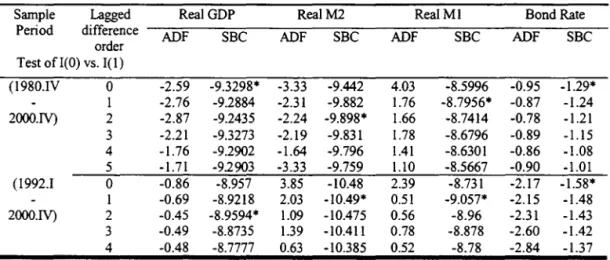
where Ut denotes the error termo Inference on (3.1) depends critically on the time series properties of mt, Yt and rt. \Ve use augmented Dickey-Fuller statistic (ADF) to test if the logarithm of Rjll. RAI2. RGDP, and rt are stationary or integrated of certain order. Because there is an issue of whether there is a structural break after the bubble burst in 1990. Table 1 reports the results of ADF using the complete sample and sub-sample period 1992.1 - 2000.1V. Both the complete sample and subsample results overwhelmingly favor the hypothesis that they are integrated of order L I( 1).

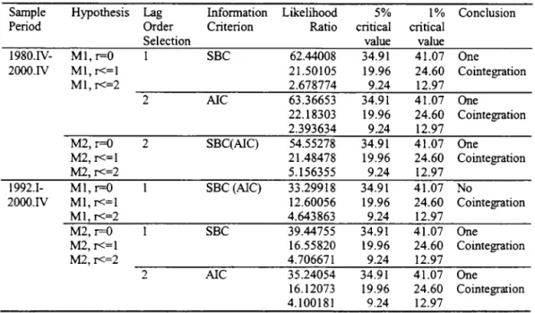
Under the assumption that mt, Yt and rt are 1(1), then the issue of whether there exists a stable money demand equation is an issue of whether there exists a cointegrating relation between mt. Yt and rt. Table 2 reports Johansen (1988. 91) likelihood ratio test results when mt, Yt and rt are alI treated as 1(1). For the complete sample period based on either AIC (Akaike (1973)) or Schwarz (1978) criterion selected order of autoregressive processo there is one cointegration between income, interest rate. and ;"11 or M2. Focusing on the subperiod of 1992.1 - 2000.1\' there is one cointegrating relation between ｾｶＱＲＮ＠ RGDP and rt but no cointegrating relation between ML RGDP and rt.

Table 3 presents the Johansen (1991) normalized cointegrating estimates between mt. Yt. and rt for both the complete sample and sub-sample period. The complete sam-pIe estimated income coeíficient for the 111 equation is exactly the opposite of what the economic theory predicts. The income coeíficient of M2 although has the correct sign, the interest rate coeíficient has the wrong signo For the subsample period, although estimates of the income coeíficients yield correct signs, they are of this unbelievable magnitude with in come elasticity of 75.23 for M1 and 11.04 for M2. Moreover, the interest rate coeíficients in these equations are of the wrong signs.

The Johansen (1991) ::VILE of the cointegrating relations is based on the decomposition of the coeíficient matrix of the leveI variables, TI, into the product of TI =

qf!.',

in an error correction representation of a vector autoregressive model where

f!'

is referred as the cointegrating relations and q is referred as the adjustment coeíficients of the deviations from the long-run equilibrium. However, as argued in Hsiao (2001a) that it is diíficult to give a structural interpretation of the cointegrating vectors

f!'

and it is preferable to view the corresponding row of TI directly as the implied long-run relation of the equation of interest. Anderson (2001) has proposed an eíficient method of directly estimating TI given the rank of cointegration. Table 4 presents Anderson's (2001) reduced rank estimation of TI assuming that there is one cointegrating relation for both the bivariate and trivariate system. They again would imply a negative relation between m and y. :-''ioreover, the

estimated coefficients are dose to zero. They appear to support the contention that there is no stable relation between money demand and income.

either the estimated long-run relation is opposite to what economic theory would predict

or it is not unreasonable to assume that the corresponding row of II is dose to zero after

1992, hence implying that there is no stable relation between money demand and income. The multivariate time series analysis is very sensitive to the time period covered

and the choice of the order of autoregressive process, p. \Ve find that either there is no

cointegrating relation between money demand and income. or if there is one, the estimated

relation is the opposite of what economic theories predict. Therefore, we turn to the single

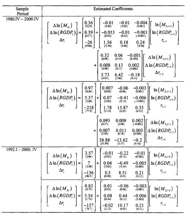
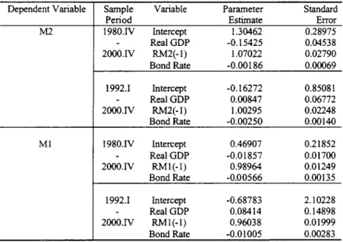
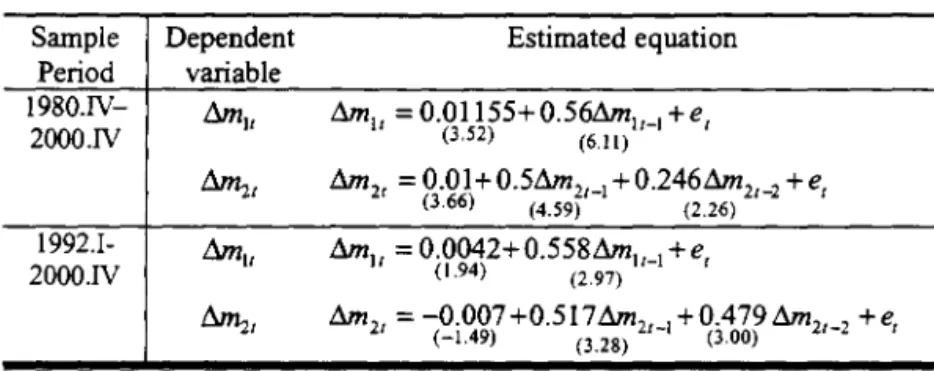
equation modeling. Table 6 presents the least squares estimates of the money demand

equation (2.3) for the period 1980.lV - 2000.lV or 1992.1 - 2000.1V. The estimated lagged dependent variable coefficient is almost exactly equal to one. The income coefficient is

either insignificantly different from zero or has the wrong signo The interest rate coefficient

is statistically significant and has the correct signo Since neither the multivariate. nor

the single equation estimates give economically meaningful interpretation of the money

demand equation. we use Box-Jenkins (1970) procedure to model the money demando Table 7 presents the ARL\!A modeling of ｾＱＱ＠ and :"12.

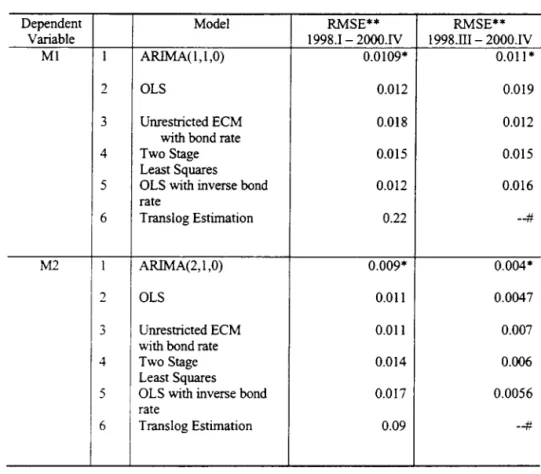
To check v·;hether the money demand equation of the form (2.3) or the univariate ARL\IA model better describes Japan's aggregate money demand, we use the prediction

principIe. As remarked by Friedman and Schwarz (1991), "the real proof of the pudding is whether it produces a satisfactory explanation of data not used in baking it - data for

subsequent or earlier years", we therefore split the sample into tv,ro periods. \Ve use data

of 1980.1\' - 1997.1V to estimate various models. \Ve then use the estimated coefficients to generate one period ahead prediction for the period 1998.1 - 2000.lV. The first column of Table 8 presents their root mean square prediction errors. The univariate ARD.IA model

predicts better than the mo deIs that also use income and interest rate as explanatory

variables.

in general favors a random walk model to a vector autoregressive or an error correction model. To gauge against unfavorable treatment of structural models, we also compare the prediction performance by using the data of 1991.III to 1998.II for estimation and generate one period ahead prediction for the period 1998.III to 2000.1V. The root mean square prediction erro r comparisons are reported at the second column of Table 8. The univariate ARIMA model again dominates the others. The fact that both the prediction results and the estimation of the form (2.3) having coefficients of lagged dependent variable almost exactly equal to one appear to support the contention that Japan's aggregate money demand is better modeled in terms of a random walk with a drift (with a drift parameter possibly changing for period after 1990).

4. Disaggregate Time Series Analysis

be obtained by slightly changing the time period covered. To get more robust estimate of the relationship between money and income. we need data to vary over a wider range. One possible way to obtain sample of greater variability is to use disaggregate time series. Japan is divided into 47 prefectures. Annual data on prefecture employee in come (the counter part to national GDP), prefecture price deflator, population statistics from 1985 -1997 are available from the home page of Economic and Social Research Institute (former Economic Planning Agency of Japan). Data on demand deposits (MF1) and MF1+ Saving Deposits (MF2) are available from Monthly Economic Statistics 01 the Bank 01 Japan. MF1 and ｾｉｆＲ＠ may be viewed as the prefecture counterpart of the national M1 and :v12 without currency held by individuaIs. (For detail, see Appendix A).

There are several advantages of using disaggregate time series. First, there are more degrees of freedom, more sample variability and less multicollinearity. Figures 1-3 plot the 47 per capita prefecture real MFL real MF2 and income over the period 1989 - 1997. The minimum and maximum prefecture logarithm of per capita real income is now 2.963 and 3.79, respectively. For the logarithm of real ::vlFL it is 0.99 and 3.44. For the logarithm of IvlF2, it is 2.65 and 4.839, respectively. The standard deviations for logarithm of per capita real income, real MF1 and real MF2 are 0.15, 0.37 and 0.34, respectively, for the sample period 1989 - 1997, and for period 1992 - 1997. the standard deviations are 0.145, 0.345,0.319 respectively. Second. it allows more accurate estimate of dynamic adjustment behavior even with a short time series. Third. it provides the possibility to control the impact of omitted variables. Fourth, it provides means to get around structural break tests which are based on large sample theory with dubious finite sample property (e.g. Hsiao (1986,2001b)).

However. there are also a number of sample and statistical issues of using prefecture data. \Ve shall first discuss issues of data measurement, then statistical modeling. finally present the empirical results.

There are three issues involved in using prefecture deposit data in domestically licensed banks. First, there is an issue of consistency of coverage of banks. There ,vas a change in the definition of banks surveyed in the deposit statistics in 1989. Due to an extension of the coverage of regional II banks in the deposit statistics in that year, the Monthly Economic Statistics of the Bank of Japan data show an unusual increase in 1989. Second, there is an issue of whether the bubble burst in 1990 created a noise that can no longer be viewed as random noise from the same population. Third, there is an issue of people living in one prefecture but working in big metropolitan prefectures, Tokyo, Osaka and Kyoto, had bank accounts near where they worked.

With the availability of panel data, it is fairly easy to check if there exist systematic measurement errors on data of some prefectures. To avoid the possibility of obtaining biased results because of inconsistent data measurements in 1989 and 1990, one may just fit a money demand equation for the year 1992 to 1997. To avoid the problem of people living in one prefecture but having bank accounts in another prefecture, we can exclude the data of Tokyo, Osaka, Kyoto, and their neighboring prefectures Chiba, Saitama, Kanagawa, and Hyogo from considerations and use the remaining 40 prefectures data to fit (2.3).

4b. Statistical Modeling

Disaggregate data focus on individual outcomes. Factors affecting individual outcomes are numerous. It is neither feasible, nor desirable to construct a model that includes all these factors in the specification. A model is not a mimic of reality. It is a simplification of reality, designed to capture the essential factors affecting the outcomes. To avoid the possibility that heterogeneity among disaggregate units might contaminate the inference of parameters of interest, model (2.3) is modified as3

b i = L ... , ｾｖＬ＠

mit = limi,t-l

+

iYjt

+

CjTt

+

aj -; Ejt,

where mit, Yit denote the logarithm of prefecture per capita real money balance and real

income, rt denotes the five year bond rate, Oi represents the prefecture specific effects that is supposed to approximate the effects of prefecture rental costs of inputs to the

praduction function of output and financiaI service and other regional specific effects. The

question of whether the coefficients ｾ＠ i

=

('li, bi , Ci)' should be assumed fixed and different

or random and different depends on whether ｾｩ＠ can be viewed as from heterogeneous

population or random draws fram a common population. In this paper we shall favor a

random coefficients appraach for two reasons: First, the short time series dimension does

not allow accurate estimation of individual ｾ＠ i' Second, if ｾ＠ i are indeed fixed and differenL the representative agent argument so frequently used by economists no longer appears

relevant. Keither is it possible to make inference about population relationship between

money demand, income, and interest rate. Therefore, we assume that the coefficients

ｾ［＠

=

(-ri, b_{i. Ci)} are randomly distributed with mean ｾ＠

=

C'?,

b,

c) and covariance matrix

ｾＮ＠ \Vhen the regional specific effects, ai, is treated as a fixed constant, we have a mixed

fixed and random effects model (Hsiao and Tahmiscioglu (1997)). \Yhen ai is treated as a

random variable that is independent of (Yit, rt) and is independently distributed across i

with mean a and variance ＨｔｾＬ＠ we have a random coefficients model (e.g. Hsiao (2001b)).

lt is well known that when regressors are exogenous the estimators based on the

sampling approach yield consistent estimates of the mean coefficients when the number

of cross-sectional units approaches infinity. However, the same results do not carry over

to dynamic models. The neglect of coefficient heterogeneity in dynamic models creates

correlation between the regressors and the error term as well as serial correlation in the

residuaIs. Keither the least squares, nor the within estimator is consistent (Pesaran and

Smith (1995)). ?v1oreover, there does not appear possible to find instruments that are

correlated with the regressors but are uncorrelated with the error termo Because there

does not appear having any consistent estimator of the mean coefficients when T is finite,

in both sma11 and moderate T samples (Hsiao, Pesaran and Tahmiscioglu (1999)) (For detail of the estimation method, see Appendix B).

4c. Empirical Results

We report the finding based on disaggregate data analysis. The first thing we wish to check is that if ｾｩ＠ are identical across i as assumed by Fujiki, Hsiao and Shen (2001). The

testing of homogeneity across i yields an F-value of 69 for ｾｉｆＱ＠ and 4.07 for MF2. Both are statistica11y significant at lo/c leveI with 40 and 117 degrees of freedom, hence rejecting the homogeneity assumption.

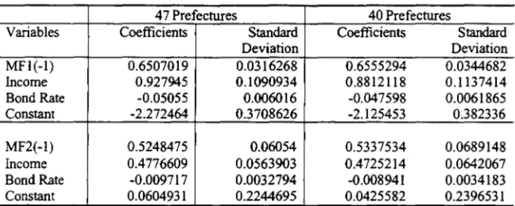
To check if the issue of people living in one prefecture but having bank accounts in another prefecture might systematically bias the estimation results, we can compare the difference between the estimates using alI 47 prefectures and the estimates based on prefecture data that are relatively free from this issue. If the systematic measurement errors are not serious, two estimates are expected to be dose. Otherwise, they are expected to be different. Tables 9 and 10 present the random coefficients and mixed fixed and random coefficients estimation ofMF1 and MF2 using alI 47 prefectures and 40 prefectures. Table 11 presents the Hausman (1978) specification test of the presence of systematic measurement errors. The chi-square statistics reject the null hypothesis ofno measurement errors at 1% significance leveI in a11 cases. We therefore concentrate our discussion based on the results using 40 prefectures.

There are three notable features arise from the disaggregate time series analysis. First, while aggregate time series analysis shows that there is no stable relation between money and income, the disaggregate time series analysis shows that there exists a stable money demand function. There is no indication that mone)' demand fo11ows a random walk with a drift.4 _{The estimated mean lagged dependent variable coefficient is significantly below}

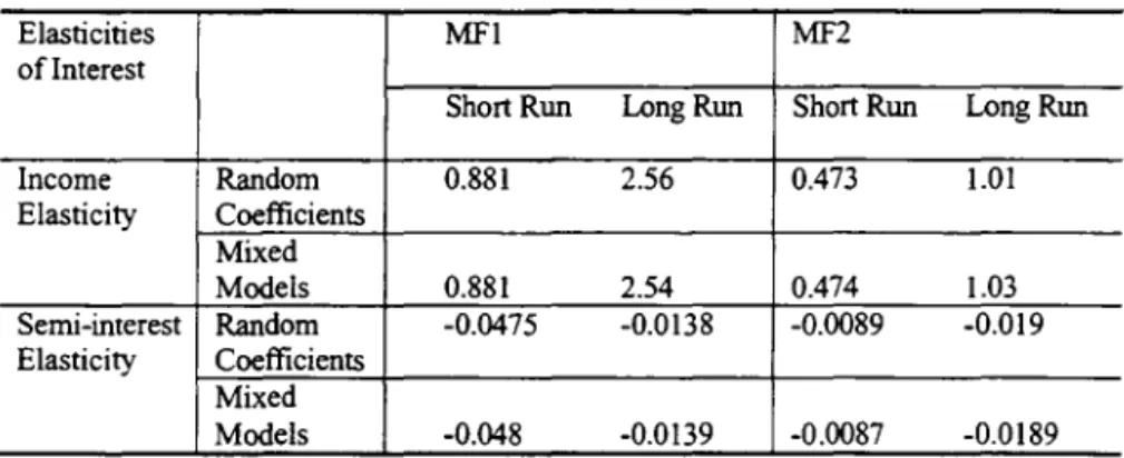
one. The mean income coefficient is positive and statistically significant. The estimated mean interest rate coefficient is negative and statistically significant. The estimated mean short-run income coefficients for 11F1 and MF2 are 0.88 and 0.47, respectiveIy. Both are Iess than 1. The estimated mean short-run interest rate coefficients for MF1 and MF2 are -0.047 and -0.009, respectiveIy.

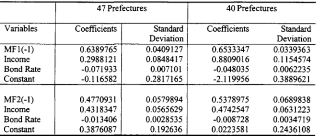
Second, the estimated mean relationship is very similar to those obtained using the formulation of Fujiki. Hsiao and Shen (2001)

i = 1. ... , _1\-, (5.1)

t = 1. ... , T,

where Di is assumed either random or fixed (see Table 12, where Di fixed or random is referred to as fixed or random effects estimator, respectively (FE or RE)). The two formulations provi de similar estimates may be due to the estimated variance-covariance matrix of ｾｩ＠ as summarized at the bottom of Tables 10 and 11 are fairly small in absolute magnitude. In other words. no matter \vhich mo deIs we use for the analysis of disaggregate data, they appear to support the contention that there is indeed a stable reIation between money demando in come and interest rate as predicted by economic theory.

Third, using the formula of ＱｾＧｙ＠ or ＱｾＧｙ＠ the estimated Iong-run in come elasticity for IvIF1 is 2.56 and for ;'IF2 is 1.01. respectiveIy for the random coefficients model and 2.54 and 1.03. respectively for the mixed random and fixed coefficients models. The Iong-run semi-interest rate for :'vIF1 is -0.138 and for MF2 is -0.019 for the random coefficients model and -0.139 and -0.0189, respectiveIy for the mixed fixed and random coefficients models. They are similar in magnitude to those obtained from the RE and FE estimates (see TabIe

N

1\-13). Csing the formula

2:::

ｬｾｩｬｩ＠ U;i or

2:::

ｬｾｩｬｩ＠ U:i, where u:, is the average weight of the

,=1 1=1

1.05. respectively, and are 2.62 and 1.06, respectively for the mixed fixed and random coefficients models.

5. Possible Source of Discrepancy

The diametrically opposite evidence obtained from the aggregate and disaggregate data series analysis makes one wonder what constitutes a well grounded leveI of analytical framework and what are the interesting interactions between disaggregate and aggregate models. In this section we explore if the issues of simultaneity, different definitions of money, and aggregation of heterogeneous units are the reasons behind this conflicting implication.

5a. Simultaneity

In a disaggregate framework it may be plausible to assume that in come and interest rate are exogenous, but the same can not be said for the aggregate data. When money, income, and interest rate are jointly determined, least squares regression of the form (2.3) yields biased and inconsistent estimates even though regressors are 1(1) (Hsiao (1997a,b)). On the other hand, two stage least squares estimator (2SLS) is consistent. Moreover, the Monte Carlo studies conducted by Hsiao and Wang (2002) have shown that despite the limiting distribution of the 2SLS of a structural vector autoregressive model is not standard normal or mixed normal when there does not exist strictly exogenous driving

force, it still doillÍnates modified estimators that possess desirable large sample properties in terms of bias, root mean square error and closeness of the actual size to the nominal size in finite sample. Therefore. we reestimate models of the form (2.3) by the two-stage least squares and present the results in Table 14. A.gain, the implication is similar to the least squares results. The in come coefficients have the wrong signs and the sums of the lagged dependent variable coefficients are almost exactly equal to one. In other words, even after taking account of simultaneity, we still can not find a stable money demand function in the 90's.

Disaggregate time series analysis uses demand deposit (MF1) and demand deposit plus time deposit (:VIF2) while aggregate time series analysis uses :VIl (currency and demand deposit) and :"12 (lvll

+

time deposit). To see if it is the component of currency holding that contributes to the lack of stable relationship between money demand and income, we redo the analysis for the (M1-currency) and (112-currency). The results of this analysis are similar to those of using M1 and M2 as the dependent variables as can be seen from the least squares and 2SLS estimates presented in Tables 15 and 16.

5c. Aggregation Over Heterogeneous l.7nits

Estimating macro relations always involves aggregation over micro units. Aggregation is valid if the disaggregate relation is linear and if all micro relations have identical param-eter values or if the distribution of the micro variables remains constant over time (e.g. Stoker (1993). Theil (1954)). Forni and Lippi (1997, 99), Hildenbrand (1994), Granger (1980). Klein (1953), Lewbel (1992, 94), Pesaran (1999), Stoker (1984, 93), Trivedi (1985), Zaffaroni (2001), etc. have shown that the dynamics of aggregate variables can be very different from the dynamics of disaggregate variables if there exists parameter heterogene-ity.

U nder the assumption of model (4.1), it is also possible to have stable micro relations but unstable macro relations. :"1odel (4.1) implies that the cointegrating relation of a prefecture takes the form

bi ci ai

mit - - - Y i t - - - r t - - - - = Vit,

1 - li 1 - -ri 1 - 1I (5.2)

N .\"

where Vit denotes a zero mean 1(0) processo Let mt =

L

mit,Yt =

L

Yit and Wit = Yit!Yt.

i=1 i=1

Then

Proposition 5.1: Tbe aggregate relatian mt - BYt - crt is 1(0) under tbe assumption

of madel (5.2) if and only if eitber

(i) Ｑｾｩｾ＠ = Ｑｾｾ＠ for all i and j and

!

li

1<

1 for all i;

.' I)

(ii) Wit = Wi for alI t and

1

li

1<

1 for ali í.

Proof: From (5.2) we have

IV b.

mt - L 'Yit

-i=l 1 - li

IV

= LVit

i=l

=

Ut·

(t

1

ｾｩｾＮＩ＠

rt -

(t

1

ＺｩｾＩ＠

i = l " i = l "

(5.3)

If the long-run reIations between mit and Yit are identical across í, then Ｑｾ［ｾ＠ _I' = ｬｾｪｾ＠ _,) =

/3,

N N N

c

=

L

1':; ., a

=

L

Ｑｾ［＠ .. Since Vit is 1(0),

L

Vt is 1(0) if alI

1

li

1<

1.

i=l i, i=l i, i=l

AlternativeIy if ｬｾ［ｩＬ＠ =1= Ｑｾ｜Ｇ＠ we can write (5.3) in the form

(5.4)

N N N

lt follows that if Wit

=

Wi for all

t,

we have.B

=

L

_ｾｗ＠ c -

L

_ｾ＠ a -

L

_ｾ＠ and i=l l - i ; " - i=l l - i , ' - i=l l - i , '

(ii) holds if

1

li

1<

1.

A sufficient condition for (i) to hold is that bi

=

b, li

=

I and

1

I

1<

1, then (5.3)

becomes

lli

mt - /3Yt - crt - a

=

L Vit,

i=l

N IV N

(5.5)

where 3

=

_b_ _{l - i '} c

=

_1_ "" C· _{l - i L..J '} and a

=

_1_ "" _{l - i L..J} a·. _, Since Vit is 1(0), so is "" _L..J Vit. In other

,=1 ,=1 ,=1

words, Proposition 5.1 states that under parameter heterogeneity there could be cases that

even though there exist stabIe reIations among micro units, the aggregate reIation can still

exhibit unit root phenomenon. For instance, if Wit =1= Wis, then

[

N bi

1

N

mt - BYt - crt - a = L

ｾｗｩｴ＠

-

/3

Yt

+

L

Vit·

i=l I' i=l

(5.6)

Even though all

1

li

1<

1, because

｛ｩｾ＠ ｬｾ［ｩ［＠

Wit

-8]

=1= O and because Yt is 1(1), mt

so that the first term on the right-hand side of (5.5) drops ouL as long as there is one ｾｩｩ＠ near 1 or equal to 1. the spectral density of (5.5) becomes unbounded. 5

Figure 4a and 4b present the distribution of,. for MF1 and MF2. The largest ,i for ｾｶｬｆＱ＠ is 0.87 for Nigata prefecture (about 2.1% ofthe total MF1 demand in 1992) and for MF2 is 0.93 for Mie prefecture (slightly above 2.4% of the total MF2 demand in 1992), hence appears to reject the hypothesis that the instability observed at the aggregate leveI is due to one of the ｾｉｩ＠ is one or near one. Figure 5 presents the distribution of Wit. They

do not appear to stay constant over time. This information appears to indicate that micro heterogeneity could be the source of discrepancy between aggregate and disaggregate.

6. A Simulation Study of the Relationship between Aggregate and Disaggregate Behavior Although in section 5 we show that ignoring parameter heterogeneity across prefec-tures could be the reason of inducing an unstable aggregate money demand function, in our micro specification (4.1) \ve use a log-linear specification. This implies that aggregation is in effect nonlinear because the aggregate variables are not defined as the sum of variables in logarithms. but are defined as the logarithm of the sum of micro variables. The nonlin-ear aggregation makes it much more difficult to derive mathematical relationships between aggregate and disaggregate relations. In this section we resort to simulation methods to show that it is indeed possible to generate unit root phenomenon and insignificant income coefficient even when there exist stable relations among micro units if the parameters are different across prefectures and the aggregation is nonlinear.

6a. The Simulation Design

\Ve artificially generate time series data for each prefecture based on the observed 5Zaffaroni (2001) shmvs that even ali,i are constrained between :0,1). as long as the tail density Of;i takes the form cb(l-'[)b with 0< Cb < x,b < Ｍｾ＠ as'[ approaches 1 from the

.\"

left. the spectral density of ｾ＠

L (1

-,;L)-lUit becomes unbounded where L denotes the

. ;=1

stylized facts. Therefore, we perform the simulation using the following steps:

1. Generate the log leveI of prefecture income using the formula: fiit = f.1i

+

Yi.t-1

+

Uit, where the drift parameter f.1i and the variance of i.i.d. error

Uit, crJ, are those derived from actual prefecture data estimates.

2. Generate bond rate using the formula: It = It-1

+

Ut, where the error term Ut is normally distributed with mean O and variances ￕＢｾ＠ equal to the variance

from the real data.

3. MF1 and :YIF2 are generated according to:

where mit denotes the log leveI of MF1 or MF2, fiit denotes the log leveI of

prefecture in come and Eit is the corresponding error term with variance equal

to the one observed at the prefecture leveI. We use the estimated random coefficients (êti,

/Ji,

1i, êi) to generate the disaggregate money demand data. The initial values for MF1 and MF2 are the prefecture leveI MF1 and MF2 at year 1992.

4. Transform the prefecture log data into leveI data. Sum the disaggregate data to get aggregate data.

6b. Results based on Simulated Aggregate Data

The estimation results based on simulated data are very similar to what we have obtained in section 3. The lagged dependent coefficients are near 1 and the income coef-ficients are either insignificant or have the wrong signo Table 17 provide the least squares estimates of the simulated 1U and M2 equation. They are of similar magnitude to those obtained from the actual data (see Table 6).

in Figures 6 and /. We also repeat the simulation by randomly assigning ｾｩ＠ to different

prefectures income data. The results are plotted in Figures 8 and 9. As one can see from

these figures the possibility of obtaining near unit root in the aggregate data is very high.

They appear to support the contention that the diametrically opposite results between the

aggregate and disaggregate analysis are largely due to ignoring heterogeneity in the micro

units in the aggregate analysis.

I. Choice between Aggregate or Disaggregate ｾｶｬｯ､･ｬ＠

Section 5 demonstrates analytically that it is possible to have stable micro relations

but unstable macro relations when heterogeneity in the micro units are present. Section 6

uses simulation to show that the diametrically opposite inferences between aggregate and

disaggregate analysis are possible with the features of money demand data observed in

J apan. Granted that there is indeed a stable relation between money demand, income and

interest rate at the prefecture leveI in Japan, the questions naturally arise are that shall

we favor using aggregate data to predict the aggregate outcomes and study the impact

of policy changes or shall we first obtain disaggregate predictions or outcomes of policy

changes, then sum the disaggregate outcomes to obtain the a&,"Tegate outcomes. In this

section we first compare the prediction performance, then compare the implication of policy

changes using aggregate and disaggregate models.

Before we compare the prediction performance between the aggregate and disaggregate

models, we note that when parameter heterogeneity is present in the disaggregate

log-linear AR(l) modeL Lewbel (1994) has shown that if the same log-log-linear form is used.

the aggregate model is of AR(::x;). since higher order lag dependent variables are not

statistically significant. we try to see if some nonlinear models would perform better than

the log-linear modeL \\Te consider three alternatives: translog (Christensen, Jorgenson

and Lau (1975)), Box-Cox transformation and inverse interest rate specifications. Tables

18, 19. and 20 present the respective estimates. The implied long-run income elasticity of

long run income elasticity is 1.33 and the implied long run interest rate elasticity is 0.058 when the logarithm of real GDP and bond rate are at the mean value of 15.28 and 1.39 respectively. However, the interest rate elasticity for j\,12 is of the wrong signo The implied

income and interest rate elasticities of Box-Cox transformation model using the procedure of Poirier and Melino (1978) yield practically zero in come and interest elasticities. For the inverse interest rate model, the long run income elasticities is 0.75 for M1 and 3.06 for .J12 and the long run interest rate elastieities are -1.3 for 1\,11 and -1.01 for M2 for the

inverse interest rate model for the full sample. For the sub sample period 1992.I-2000.IV, the inverse of bond rate coefficients are not significant and logarithm of real GDP has the wrong signs. Moreover, the lagged dependent coefficients both exceed 1. Therefore we cannot draw consistent conclusion about the long-run relations based on the inverse of interest rate for both full sample and subsample periods.

The nonlinear models not only may imply implausible ineome and interest rate elas-ticities. they also have statistically insignificant parameter estimates for the higher order terms. r-Ioreover. neither do the nonlinear mo deIs predict better than AREvfA or log-linear model (see Table 8). Therefore, for the aggregate models we shall foeus our comparison using only ARüL-\ or model (2.3).

In choosing between whether to predict aggregate variables using aggregate or disag-gregate equations (Hd ). Grunfeld and Griliches (1960) suggest using the criterion of:

Choosing Hd if ｾ､ｾ､＠

<

ｾｾｾ｡Ｇ＠ otherwise choosing Ha,

where ｾ､＠ and ｾ｡＠ are the estimates of the errors in predicting aggregate outeomes under H d and Ha, respecti\"ely. Table 21 presents the within sample fit eomparisons in the

first row and the post-sample prediction comparison in the second roW. Both criteria unambiguously favor predicting aggregate outcomes by summing the outcomes from the disaggregate equations.6

\Ve next perform simulation studies to evaluate the impact of changing interest rates

on the aggregate money demand using either the macro or the disaggregate equations.

\Ve shock the economy by lowering the interest rate for 50% and observe the evolution

of the money demand at the prefecture leveI and then get aggregate money demand from

the prefecture money demando The prefecture money demand is modeled by the random

coefficient model specified in (4.1). To use the macro equations to evaluate the interest rate

shock impact, we assume that we have available only the aggregate data that have been

constructed form the prefecture leveI and have no information about how the prefecture

leveI data are generated.

\iV-e need to construct three aggregate senes through simulation study. First. the

'·true aggregate series" before and after the interest rate shock. Again we simulate the

disaggregate data using all stylized facts from the actual Japan's money demand data. and

we shock the disaggregate system at period T=101, which gives interest rate as half of its

leveI at T=100.

Secondly, assume that we don't know the existence of the disaggregate equations but

only have the final simulated 100 periods of aggregate data, we use these observation points

to perform OLS estimation and use the estimated coefficients to evaluate the response of

this aggregate system to interest rate shock and we call it "simulated aggregate response".

Finally. we construct the "simulated aggregate response from disaggregate equations"

from the micro data by first estimating a random coefficients model using data of first 100

periods then using the estimated coefficients to construct prefecture leveI money demand

after the interest rate shock, and aggregating them to obtain the estimated aggregate

response.

The error sum of squares for predicting true system's responses after interest shock is

much smaller for the disaggregate system as compared to aggregate system. For a typical

simulation, the error sum of square for M1 from disaggregate system is at the magnitude of 5.88*lOi, and that from aggregate system is 2.51*1010 ; the error sum of square for M2 for the disaggregate system is at the magnitude of 2.04

*

1043_{, and that from the aggregate}

system is 9.55*1045 . As the absolute nurnbers of the error sum of squares are very large, we further look at the responses paths from the disaggregate and aggregate system.

Figure 10 contains the changes of both the "true aggregate series" and "simulated disaggregate responses", with the dashed line shows the simulated disaggregate responses and the solid line shows the "true aggregate responses". The top two figures are for M1 and the bottom two are for M2, and the left half shows the short run responses while the right half shows the long run responses. This figure shows that the series of the "true aggregate series" and the simulated disaggregate responses are very similar. Both lines show increase of money demand in the short run and then converge to certain equilibriurn level in the long run.

Figure 11 plots the responses of both the macro equations and the disaggregate equa-tions together with the "true aggregates". Again the top two figures are for A11 and the bottom two figures are for 1v12, and the left two figures show the short run responses while the right two figures show the long run responses. The two very dose lines denote "true aggregates (solid line)" and "aggregates from the disaggregate equations (dashed line)", respectively, and the third dashed line denotes "the macro equation response". These fig-ures shmv that summing the micro responses to get the aggregates is dose to the true ones but the macro equation responses are very different from the true ones. Because af the

near unit raat phenomenan in the aggregate ma deI even thaugh the estimated shart-run

interest elasticity is small, it wauld almast imply the presence af "liquidity trap" in the lang-run.

mo deI to generate aggregate outcomes ..

8. Conclusions

In this paper we study the issues of whether Japan has a stable money demand function under the low interest rate policy using both aggregate and disaggregate data. There are two notable results. First, the only agreeable information is that the interest rate coeflicients although are statistically significant, they are not of the magnitude to imply the presence of liquidity trap in the short run. \Ve have here mostly only reported findings in terms of semi-Iog form for the interest rate. We have tried alternative functional forms for the interest rate such as logarithmic transformation or the inverse transformation. Both specifications could imply the presence of liquidity trap if the estimated coeflicients have the right magnitude. However, the alternative functional forms do not fit the data or yield post-sample prediction as well as the semi log form reported here. The panel data estimated short-run semi-interest rate elasticity based on random coeflicient models is -0.048 for MF1 and -0.009 for :VlF2. The long-run interest elasticities are -0.139 for MF1 and -0.019 for 1IF2.

a real M2 growth rate of 7.36%. The real growth rate of GDP during this period is 4.13%. Had interest rate stayed constant, the ratio of these two numbers, 1. 78, gives a measure of long-run in come elasticity of the demand for real M2. In the 90's, the average growth rate of M2 is 2.69%, the infiation rate is 0.14%. The real growth rate of M2 is about 2.55%. The real GDP growth rate during this period is 1.38%. The ratio of real growth rate of M2 and real GDP is about 1.85. Taking account of the fact that 1.78 or 1.85 is the average measure assuming interest rate stayed constant, while in fact the five year bond rate had fallen from 9.332 at 1980.1 to 5.767 at 1989.1V and further to 1.289 at 2000.lV and the estimated impact of interest rate changes on money demand, these figures are indeed very dose to the estimated long-run in come elasticities based on disaggregate data analysis.

\Ve have also tried to explore the source of the seemingly contradictory evidence between the aggregate and disaggregate data. It appears that the lack of stable relationship between aggregate money demand and income could be due to the lack of sample variability in the aggregate data. But more importantly, our analytical and simulation results appear to suggest that it is the ignoring of heterogeneity in the micro units and the effect of nonlinear aggregation that lead to this seemingly contradictory evidence. In other words, our empirical analysis appears to suggest that more attention should be directed at the issues of aggregation and more structure is needed to justify aggregate data models. The results shm" that it is possible to have stable micro relations but unstable macro relations.

Appendix A: Definitions of Disaggregate Data

This appendix explains the definitions of prefecture income statistics, population and the prefecture money aggregates.

1. Prefecture income statistics

Prefecture in come statistics complied by the Economic and Social Research Insti-tute (Former Economic Planning Agency of Japan) for each fiscal year provi de a good counter part to national GDP. We dO\\TIload the data from the home page of Economic and Social Research Institute from 1987 - 1997, and supplement the data of 1986 - 1997 from Fujiki and :Mulligan (1996).

The prefecture in come data is deflated by the gross prefecture expenditure defla-tor during the period from fiscal year 1985 to fiscal year 1997.

2. Population

We use population to convert prefecture data to per capita data. The population of each prefecture is as of the beginning of October of each year.

Prefecture Money Aggregates

l. ｾｉｆＱ＠

:vIF1 is the end of month outstanding demand deposits held by individuaIs and firms at domestically licensed bank. ｾｉｆＱ＠ data by prefecture are available from

Monthly Economic Statistics of Bank of Japan. Due to the extension of the cov-erage banks included in this statistics in April1989 and occasional consolidations of banks, MF1 data sometimes show an unusual increase. particularly in April 1989.

amount of currency heId by individuals are not avaiIabIe. Second, they do not have the breakdown by the individuals and firms. Third, they do not include the demand deposit at the community banks, the Norinchukin bank, and the Shokochukin bank, which are included in the computation of the :\U statistics. However, :'-lF1 data aIways expIain about 70 percent of M1 during 1985 - 1998, and about 80 percent from 1989 - 1991, and about 70 percent from 1992 to 1997. Therefore, :vlF1 predicts about 70 percent of M1 for 1991 - 1997, the period covered in the disaggregate time series analysis.

2. :\IIF2

MF2 is the sum of the deposit in domestically Iicensed banks, community banks and Shokochukin Bank. MF2 consists ofboth demand deposit and savings deposit and is our counterpart of national M2

+

CD minus cash, with the existence of the following statistical discrepancies:

First, the prefecture breakdown of CDs outstanding does not exist, hence we ignore them. Second, we only eIiminate the deposit heId by the financiaI insti-tutions for domestically licensed banks, since the breakdown of deposits heId by financial institutions by prefecture are avaiIabIe for domestically licensed banks only. Third, we exclude the data for the Xorinchukin bank from the regional deposit statistics to avoid possible double count of same deposits. However, MF2 data aIways expIain about 98 percent of :'-12

+

CD from 1985 - 1998, about 95 percent from 1993 - 1995, and about 90 percent from 1996 - 1997. Therefore, MF2 predicts aImost constant proportion of M2

+

CD when we are careful about the seIection of sampIe period.

Appendix B: Hierarchical Bayes Estimation of Random Coefficients and :vExed Fixed and Random Coefficients Models

In this appendix we explain how the random coefficient models and the mixed fixed and random coefficients models are estimated in the Bayesian framework. \Ye start with a general framework by Hsiao, et.al (1993), and then explain how this general framework is implemented in trus paper.

Suppose there are observations of 1

+

kI

+

k2 variables (Yit, f:t, ｾＺｴＩ＠ of N cross-sectional units over T time periods, \vhere i = L ... , }\[ and t = 1, ... , T.

Denote

where

y' (YiI .... , YiT),

-I

1 x T

Zi

'T X k2

i = L ... ,.\T. vYe assume that

(B.l)

where;3 and -: are

-

-

SkI x 1 and Xk2 x 1 vectors respectively, and

1!

, ( ) E( ') { crPT

ｾｩ］＠ Uil,···,UiT. ｾｩｕｪ＠ =

o

if _if Z _i = J,

-1= j.

We further assume that the Nkl x 1 vector (3 satisfies:

q

ｾ＠

l:J

ｾ＠

A,

ｾ＠

+

2

(B.3)

where ｾｩ＠ is kl X 1 vector, i = 1, ... , 1V, AI is an Nk1 x m matrix with known elements,

7J

is an m x 1 vector of constants, and

2 -

N(Q,C)'2

ｾ＠

l:J

(B.4)

and the variance covariance matrix C is assumed to be nonsingular, and E(TJ·)

-.

= Q, E(TJ .TJ')

_-

=

,-)

ｻ

ｾ＠ if i=j

º

if i -1= j .

The N k2 x 1 vector of I is assumed to satisfy

1=

Ｈｾｬ＠

)

=

A27N'

IN

(B.5)

where A2 is an Nk2 x n matrix with known elements, and

i

is an n x 1 vector of constants.

Because A2 is as known matrix, (B.1) is formally identical to

(B.1')

where

Z

= ZA2 . However, by postulating (B.4) we can allmv for various possible fixed parameter configurations.

B.I. Formulation and estimation of dynamic random coefficient models.

If we let

m (B.1), where F::N denotes the 1"; x 1 vector of ones, we get random coefficients model

with

ifi

=

ｑｩｾＫｲｩＬ＠ i

=

L ... ,1\:, (B.7)

where Qi = (ifi,_l'Xi ), ｾｩ＠ includes the coefficient for lagged dependent variable

Jf.i,-l

=

(YiO, ... , Yi,T-d', and ?2i = Qi"li

+

ｾｩＧ＠ (B.8)

\Ve change notation Xi to Qi = (ifi,-l' X;) to emphasize that the present model is a

dy-namic one, where Xi denotes all the exogenous explanatory variables. As a result of the

dynamic feature ofthe present model, E(1:::i

I

Q;) =1= O (Hsiao (2001b)). Therefore, contrary

to the static case, the least squares estimator of the common mean, ｾ＠ is inconsistent. In addition, the covariance matrix of 1/i, F, is not easily derivable, hence the procedure of

premultiplying (B.8) by lc-1 !2 to transform the model into one with serially uncorrelated errar is not implementable. :\'either the Instrumental Variable method appears

imple-mentable as the instruments that are uncorrelated with 1::: i are most likely uncorrelated

\vi th

Q

i as well.

Our estimation procedures use the Hierarchical Bayes Estimator developed by Hsiao,

Pesaran and Tahmiscioglu (1999).

This estimatar is performed in the following steps:

Step 1: 'C nder the assumption that YiO are fixed and known and TI and Uit are

inde--I

pendently normally distributed. we can implement the Bayes estimator of ｾ＠ conditional

on

cr[

and .6. using the formula for the (unconditional) posterior distribution ｯｦＮｾ＠ given if

(Hsiao eLal (1993. p,IO)).

The Bayes Estimator conditional on .6. and

crf

is:

!

B =

{:t

(crf

(Q;Q;)-l

+

6.)-1} -1

L[crf(

Q;Qi)-l

+

.6.

r

1

ｾｩＧ＠

1=1 1=1

0-;

｡ｮ､ｾＺ＠

The above steps give empirical Bayes Estimator. We save the estimated

li

and the related variances to construct the informative prior for the Hierarchical Bayes Estimator.

Step 2: Use Gibbs Sampler to Calculate the Hierarchical Bayes Estimator.

Assume that the prior distribution of

ur

and ｾ＠ are independent and are distributed as

where VV represents the \Vishart distribution with scale matrix pR and degrees of freedom (p) (Lindley and Smith (1972)). Incorporating this prior into (B.7) and (B.8), we use Gibbs sampler to calculate marginal post error densities of the parameters of interest by integrating out

ur

and .6. from the joint posterior density.

The Gibbs sample is an iterative Markov Chain Monte Carlo method which only re-quires the knowledge of the full conditional densities of the parameter vector (e.g. Gelfand and Smith (1990)). Starting from some arbitrary initial values, say ＨｾｩｏＩＬ＠ ｾｾｏＩＬ＠ ... , _{ｾｫｏﾻＩ＠} for a parameter vector ｾ＠ = ＨｾＱＢＢ＠ ＧｾｫＩＧ＠ it samples alternatively from the conditional density of each component of the parameter vector conditional on the v-alues of other components sampled in the latest iteration. That is:

(1) S _ampe 1 eCi+l) _-1 f _rom p(e _{_1}

I

eU) eU) _{-2 '-3 ""'-k} eU»)

_'I!

(k) S 1 eCi+l) f p(e

I

eCi+1_{) eU+}1_») ampe -k rom _k -1 " " ' - k - l

'I!

stage ｾＨｪＩ＠ to the next stage ｾＨｪＫＱＩ＠ being

ｋＨｾＨｪＩＬｾＨｪＫＱﾻＩ＠ = _{ｐＨｾｬ＠} I _{ｾｾｪＩＬ＠} ... ＬｾｾｪＩＬ＠ .... ｾｾｪＩＧＡｦＩｐＨｾＲＱ＠ ｾｩｪＫｉＩＬｾｾｪＩＬ＠ ... ＬｾｾｪＩＬｹＩ＠

( Ll

I

Ll(j+1) Ll(j+1»)

... P fZk fZ1 , ... ,fZk-1 ,!f'

As the number of iterations j approaches inflnit)", the sample values in effect can be re-garded as drawing from true joint and marginal posterior densities. :vloreover, the ergodic averages of functions of the sample values will be consistent estimation of their expected values.

In our case, ｾ＠ i is ｾ＠ i' C nder the assumption that the prior of ｾＬｩｲＬ＠ and the related variances lJI are obtained from Empirical Bayes Estimator, the Gibbs sampler for (B.6) -(B.7) are easily obtained from

P(6. -,

I

ｾＮＸＬ＠

•...•

;3".

￣Ｌ｡ｾＮＮＮ＠

a,,)

-

W [

(t,(q,

-

ｾＩＨ￢Ｌ＠

-

ar

+

PR)

-, ,

P

+

N

1

P(af

I

!fi' li1"" ＬｬｩｳＧｾＧＮＶ＠ -1) '" IG[T/2, (!fi - ｑｩｾｙＨＡｦｩ＠ - Qilii)/2], i

=

1, ... , S,

A .v

v.-here Ai = ＨＨ｡ｩＲｑｾｑｩ＠

+

.6-1 )-1,D = (S.6.-1

+

1JI-1)-1,/3 _{_} =

+

_-

L:

8, and _{_ z} IG denotes .=1

the inverse gamma distribution.

2. Mixed Fixed and Random Coeflicient Models.

(B.3) and (B.l') gives the mixed fixed and random coeflicient model used by Hsiao et.al, (1989) and Hsiao and Tahmiscioglu (1997).

The estimator could have followed the Bayesian estimators by Hsiao et.al (1993). However, as diffuse priors are assumed for ｾ＠ in this framework, while Gibbs samples works under informative priors (using diffuse prior fails to converge to the right distribution

References

Akaike, H., (1973). "Information Theory and an Extension of the Maximum Likelihood PrincipIe." in Proc. 2nd int. Symp. lnformation Theory, ed. by B.:VI. Petrov and F. Csaki, 267-281, Budapest: Akademiai Kiado.

Anderson, T.W., (2001). "Reduced Rank Regression in Cointegrated Models," Journalof Econometrics, (forthcoming).

Bernanke, B.S. (2001), "Japanese ｾｬｯｮ･ｴ｡ｲｹ＠ Policy: A Case of Self Induced Paralysis?" in Ryoichi Mikitaui and A.S. Posen, Eds., Japan's Financial Crisis and its Parallels to U.S. Experience, Institute for International Economics, Bank of Japan.

Bohn, H .. (1995). "The Substitutability of Budget Defieits in a Stochastie Eeonomy,"

Journal of Money, Credit and Banking, 27, 257-271,

Box, G.E.P. and D.R. Cox (1964). "An Analysis of Transformations," Journal of the Royal Statistical Society. Series B, 26, 211-252.

Box. G.E.P. and G.M. Jenkins (1970). Time Series Analysis, Forecasting and Control, San

Francisco: Holden Day.

Brewer. K.R.\V. (1973), "Some Consequences of Temporal Aggregation and Systematic Sampling for ARIMA and AR:vlAX Models," Journal of Econometrics, 1, 133-154.

Christensen, 1., D.W. Jorgenson and 1.J. Lau (1975). "Transcendental Logarithmic utility Functions" American Economic Review. 65, 367-83.

Diekey, D.A. and W.A. Fuller (1979). "Distribution of the Estimators for Autoregressive Time Series with a unit Root." Journal of the American Statistical Association, 74,

427-431,

_--::-:-.,...--,=-_, (1981). ;'Likelihood Ratio Statisties for Autoregressive Time Series with a "C'nit Root," Econometrica, 49. 1057-1072.

Doi. T .. (2000). "Wagakuni ni okera Kokurai no Jizokukanousei to Zaiser enei," in Ihori et aI. "Zaisei Akazino Keiza: Bunsehi: Cvu-cvokiteki Shiten karano Kousatsu." Keizai-bunseki Seisaku kenkyu ｮｾ＠ Shiten ｓ･ｲｩｾｳＬ＠ \;01. 16, 9-15. .

Forni, :vI. and ;vI. Lippi (1997). Aggregation and the Microfoundations of Dynamic Macroe-conomics, Oxford: O>..'ford C niversity Press.

__ ＭＭ［ＺＭｾＭＭＺＭＺＭ｟＠ (1999). "Aggregation of Linear Dynamie :vlieroeconomics Models," Journal of Mathematical Economics, 31, 131-158.

Friedman, M. and A.J. Schwartz, (1991). "Alterative Approaches to Analyzing Economie Data." American Economic Review, 81, 39-49.

Fujiki. H., (2001). ":vloney Demand Near Zero Interest Rate: Evidence from Regional Data." mimeo.

----=:-:--0---7' C. Hsiao and Y. Shen (2002). "Is there a Stable Money Demand Function

Economic Studies, Bank of Japan, (fortheoming).

_----::::---_-:-::- K. Okina, and S. Shiratsuke (2001). "Monetary Poliey Under Zero Interest Rate: Viewpoints of Central Bank Eeonomists," Monetary and Economic Studies, 19,

s-1,89-130.

Gelfand, A.E. and A.F.M. Smith (1990). "Sampling-Based Approaehes to Caleulating :Marginal Densi ties," 85, 398-409.

Granger, C.W.J. (1980). "Long Memory Relationships and the Aggregation of Dynamic :'1odels," Joumal

01

Econometrics, 14, 227-238.

Grunfeld, Y. and Z. Griliehes (1960). "Is Aggregation Neeessarily Bad?," Reuiew

01

Eco-nomics and Statistics, 42, 1-13.

Hausman, J.A., (1978). "Speeifieation Tests in Eeonometrics," Econometrica, 46,1251-71.

Hobert, J.P., Casella, G. (1996). "The Effeet of Improper Priors On Gibbs Sampling in Hierarehieal Linear Mixed Models," Journal

01

the American Statistical Association,

91, 1461-1473.

Hsiao,

C.,

(1986). Analysis

01

Panel Data, Eeonometrie Soeiety monographs No. 11, New

York: Cambridge University Press.

__ -:::-___ , (1997a). "Cointegration and Dynamie Simultaneous Equations Models,"

Econometrica, 65, 647-670.

｟ＭＭＺｾＭ［ＭＭＭＺＢＧＢＧＢＧ＠ (1997b). "Statistieal Properties of the Two Stage Least Squares Estimator Cnder Cointegration," Reuiew

01

Economic Studies, 64, 385-398.

_--:--::--_-;;, (2001a). "Identification and Diehotomization of Long- and Short-Run Re-lations of Cointegrated Vector Autoregressive Models," Econometric Theory,

17,889-912.

_ _ -=-:-_-:--:_, (2001b). "Eeonomic Panel Data Methodology," in Intemational Encyclope-dia

01

the Social and Behauioral Sciences, ed. by N.J. Snelser and P.B. Bates, Oxford:

EIsevier. (fortheoming).

_ _ --:;-=:--and A.K. Tahmiseioglu (1997). "A Panel Analysis of Liquidity Constraints

and Firm Investment," Joumal

01

the American Statistical Association, 92, 455-465.

ＭＭＭＺ［ＺＺｯＭＭＭＺ［ＺＺ［Ｍｾ＠ M.H. Pesaran and A.K. Tahmiseioglu (1999). "Bayes Estimation of Short-Run Coeffieients in Dynamie Panel Data Models," in Analysis

01

Panels and Limited Dependent Variables Models, ed. by C. Hsiao, L.F. Lee, K. Lahiri and M.H. Pesaran,

Cambridge: Cambridge University Press, 268-296.

- - - - 7 " " : : : - and S. Wang (2002). "Estimation of Struetural Vector Autoregressive

Inte-grated Proeess," mimeo.

Johansen, S., (1988). "Statistieal Analysis of Cointegration Veetors," Journal

01

Economic Dynamics and Contral, 12, 231-254.

Klein. L.R. (1953). A Textbook of Econometrics, Evanston: Row Peterson and Company.

Laidler, D.E.\,y., (1969). The Demandfor Money: Theories and Evidence, Scranton, Penn:

International Textbook Company.

LewbeL A. (1992). "Aggregation with Log-Linear Models," Review of Economic Studies,

59, 635-642.

_ _ ::---=-::-:---::-(1994). "Aggregation and Simple Dynamics," American Economic Review, 84, 905-918.

Lindley, D.V. and A.F.M. Smith (1972). "Bayes Estimates for the Linear ModeL" Journal of the Royal Statistical Society, B. 34, 1-41.

:-'-akashima, K., and M. Saito (2000). "Strong Money Demand and Nominal Rigidity: E,,:idence from the J apanese Money Market C nder the Lo\\" Interest Rate Policy,"

mzmeo.

:.'\erlove, M., (1958). The Dynamics of Supply: Estimation of Farmers' Response to Price,"

Baltimore. the John Hopkins Press.

Pesaran, ｾＱＮｈＮ＠ (1999). "On Aggregation of Linear Dynamic rvIodels," mimeo.

_---,=-___ and Smith (1995). "Estimation of Long-Run Relationships from Dynamic Heterogeneous Panels," Journal of Econometrics, 68, 79-114.

_---,,--....,---=:=-, R.G. Pierse and 1-1.5. Kumar (1989), "Econometric Analysis of Aggregation in the Context of Linear Prediction ｾｉｯ､･ｬｳＩＩＬ＠ Journal of Econometrics 57, 861-888.

Poirier, D.J. and A. Melino (1978). "A Note on the Interpretation of Regression CoefE.-cients \Vithin a Class of Truncated Distributions," Econometrica, 46, 1207-1209.

5chwarz, G. (1978). "Estimating the Dimension of a :ModeL" Annals of Statistics, 6,

461-464.

Stoker, T .:M. (1984). "Completeness, Distribution Restrictions, and the Form of Aggregate Functions." Econometrica, 52, 887-907.

__ -:-;,.--.,--,,- (1993). "Empirical Approaches to the Problem of Aggregation Over Indi-viduaIs," Journal of Economic Literature, 31, 1827-1874.

Theil. H. (1954). Linear' Aggregation of Economic Relations. Amsterdam: :.'\orth Holland.

Tiao G.C., (1972). "Asymptotic Behavior ofTemporal Aggregates ofTime Series." Biometrika.

59. 525-531.

Trivedi. P.K. (1985). "Distributed Lags, Aggregation and Compounding: Some Econo-metric Implications." Review of Economic Studies, 52, 19-35.

Table 1 ADF Tests ofUnit Roots a.b

Sample Lagged RealGDP RealM2 RealMI Bond Rate

Period difference _{ADF SBC ADF SBC ADF SBC ADF SBC}

order Test ofI(O) vs. l(l)

(1980.lV O -2.59 -9.3298* -3.33 -9.442 4.03 -8.5996 -0.95 -1.29*

I -2.76 -9.2884 -2.31 -9.882 1.76 -8.7956* -0.87 -1.24

2000.1V) 2 -2.87 -9.2435 -2.24 -9.898* 1.66 -8.7414 -0.78 -1.21

3 -2.21 -9.3273 -2.19 -9.831 1.78 -8.6796 -0.89 -1.15

4 -1.76 -9.2902 -1.64 -9.796 1.41 -8.6301 -0.86 -1.08

5 -1.71 -92903 -3.33 -9.759 1.10 -8.5667 -0.90 -1.01

(1992.1 O -0.86 -8.957 3.85 -10.48 2.39 -8.731 -2.17 -1.58*

I -0.69 -8.9218 2.03 -10.49* 0.51 -9.057* -2.15 -1.48

2000.1V) 2 -0.45 -8.9594* 1.09 -10.475 0.56 -8.96 -2.31 -1.43

3 -0.49 -8.8735 1.39 -10.411 0.78 -8.878 -2.60 -1.42

4 -0.48 -8.7777 0.63 -10.385 0.52 -8.78 -2.84 -1.37

The * indicates the optimally selected lag order.

Table 2 Johansen Likelihood Ratio Test Results When Ml (M2), GDP and Bond Rate are 1(1)

Sample Hypothesis Lag Infonnation Likelihood 5% 1% ConcIusion Period Order Criterion Ratio criticai criticai

Selection vaIue value

I 980.IV- MI,r=O I SBC 62.44008 34.91 41.07 One 2000. IV MI, r<=1 21.50105 19.96 24.60 Cointegration

MI, r<=2 2.678774 9.24 12.97

2 AlC 63.36653 34.91 41.07 One

22.18303 19.96 24.60 Cointegration 2.393634 9.24 12.97

M2, r=O 2 SBC(AlC) 54.55278 34.91 41.07 One

M2,r<=1 21.48478 19.96 24.60 Cointegration

M2,r<=2 5.156355 9.24 12.97

1992.1- MI, r=O SBC (AlC) 33.29918 34.91 41.07 No

2000. IV MI, r<=1 12.60056 19.96 24.60 Cointegration

MI, r<=2 4.643863 9.24 12.97

M2, r=O SBC 39.44755 34.91 41.07 One

M2, r<=1 16.55820 19.96 24.60 Cointegration

M2,r<=2 4.706671 9.24 12.97

2 AlC 35.24054 34.91 41.07 One

Table 3 Johansen (1991) Nonnalized Cointegration Vector

*

1980.IV - 2000.lV 1992.1 - 2000.IV

MI M2 MI M2

Basedon SBe

GDP -0.72 3.83 7523 8.225

(-1.337) (3.34) (258) (8.27)

BondRate -0.13 0.108 2.666 0.316

(0.079) (0.17) (9.92) (0.41)

Intercept -26.43 -4429 -1156 -112.7

(21.22) (53.54) (4017) (129.3)

Basedon Ale

GDP 0.183 Sameas Sameas 11.036

(0.674) SBe SBe (12.33)

Bond Rate -0.05 0.404

(0.049) (0.552)

Intercept -17.62 -156.4

(10.59) (192.4)

Table 4 Anderson's (2001) Reduced Rank Estimation

Sample Monetary Period Al!l!Tel!ates

1980.1 V- 2000.IV MI

M2

1992.1 - 2000.IV MI

M2

• TI is the long run coefficient matrix in

[

B

P IIp

+

L

B21p

p=1 B 31p

The Long Run Coefficient TI

[-0.0004 -0.0002 0.0645] -0.0010 -0.0006 0.1523 -0.3178 -0.177548.0654

[-0.0007 -0.00040.0645] -0.0013 -0.00080.1195 -0.5535 -0.341549.697

[ 0.0026 0.0004 0.0376] 0.0193 0.0031 0.2741 2.1893 0.3468 31. 1393