www.solid-earth.net/7/1157/2016/ doi:10.5194/se-7-1157-2016
© Author(s) 2016. CC Attribution 3.0 License.
Archie’s law – a reappraisal
Paul W. J. Glover
School of Earth and Environment, University of Leeds, Leeds, UK
Correspondence to:Paul W. J. Glover ([email protected])
Received: 7 March 2016 – Published in Solid Earth Discuss.: 5 April 2016 Revised: 31 May 2016 – Accepted: 15 June 2016 – Published: 29 July 2016
Abstract.When scientists apply Archie’s first law they often include an extra parameter a, which was introduced about 10 years after the equation’s first publication by Winsauer et al. (1952), and which is sometimes called the “tortuosity” or “lithology” parameter. This parameter is not, however, the-oretically justified. Paradoxically, the Winsauer et al. (1952) form of Archie’s law often performs better than the origi-nal, more theoretically correct version. The difference in the cementation exponent calculated from these two forms of Archie’s law is important, and can lead to a misestimation of reserves by at least 20 % for typical reservoir parameter val-ues. We have examined the apparent paradox, and conclude that while the theoretical form of the law is correct, the data that we have been analysing with Archie’s law have been in error. There are at least three types of systematic error that are present in most measurements: (i) a porosity error, (ii) a pore fluid salinity error, and (iii) a temperature error. Each of these systematic errors is sufficient to ensure that a non-unity value of the parametera is required in order to fit the elec-trical data well. Fortunately, the inclusion of this parameter in the fit has compensated for the presence of the systematic errors in the electrical and porosity data, leading to a value of cementation exponent that is correct. The exceptions are those cementation exponents that have been calculated for individual core plugs. We make a number of recommenda-tions for reducing the systematic errors that contribute to the problem and suggest that the value of the parametera may now be used as an indication of data quality.
1 Introduction
In petroleum engineering, Archie’s first law (Archie, 1942) is used as a tool to obtain the cementation exponent of rock units. This exponent can then be used to calculate the
vol-ume of hydrocarbons in the rocks, and hence reserves can be calculated. Archie’s law is given by the equation:
ρo=ρfφ−m, (1)
whereρo is the resistivity of the fully water-saturated rock sample,ρf is the resistivity of the water saturating the pores, φ is the porosity of the rock, m is the cementation expo-nent (Glover, 2009), and the ratioρo/ ρf is called the for-mation factor. Archie’s law in this form was initially empiri-cal, although it was recognised that certain values of the ce-mentation exponent were associated with special cases that could be theoretically proven. Glover (2015) provides a re-view. Later, this form of Archie’s law would be given a bet-ter theoretical grounding by being derived from other mixing models.
However, at least nine out of ten reservoir engineers and petrophysicists do not use Archie’s first law in this form. In-stead, they use a slightly modified version which was intro-duced 10 years later by Winsauer et al. (1952), and which has the form:
ρo=aρfφ−m, (2)
whereais an empirical constant that is sometimes called the “tortuosity constant” or the “lithology constant”. In reality, the additional parameter has no correlation to either rock tor-tuosity or lithology and we will refer to it as theaparameter (Glover, 2015).
is not valid for rocks with porosities approaching the limit φ→1. This incompatibility that Eq. (2) has with its lim-iting value leads to the idea that Eq. (1) is a better qual-ity model than Eq. (2), which has some intrinsic problems. While the fact that Eq. (2) breaks down when approaching the limit φ→1 would not necessarily cause a petrophysi-cist to be concerned, the question ought to arise whether the Winsauer et al. (1952) modification to Archie’s first law is valid within the range in which it is usually used. Since the Winsauer et al. (1952) modification to Archie’s first law usu-ally produces better fits to the experimental data, its validity is not questioned further and the practice of applying Eq. (2) and obtaining a non-unity value for theaparameter remains common practice within the hydrocarbon exploration indus-try.
While most scientists fit Eq. (2) to measurements made on a group of data from core plugs from the same geological unit or facies type on a log formation factor vs. log poros-ity plot, some petrophysicists prefer to calculate cementation exponents for individual core plugs than calculate a mean and standard deviation for a given group of measurements. This approach has been considered justified (e.g. Worthing-ton, 1993), but runs the risk of including samples from more than one facies type by accident or oversight, whereas the use of a plot allows the uniformity and relevance of the data from all of the samples to be judged during the derivation of the cementation exponent. Moreover, plug-by-plug calcu-lation of the cementation exponent is carried out with the equation:
m= −logF /log φ, (3)
which includes noa parameter, being derived from Eq. (1). Consequently, plug-by-plug calculation of mean cementation exponent and that derived from graphical methods are often disparate.
The rest of this paper examines the apparent paradox that whereas Eq. (1) has a longer and theoretically better pedi-gree, Eq. (2) is the version that is overwhelmingly more com-monly applied because it fits experimental data better. We show that, while the original Archie’s law is the most cor-rect physical description of electrical flow in a clean porous rock that is fully saturated with a single brine, the Winsauer et al. (1952) variant is the most practical to apply because it compensates to some extent for systematic errors that are present in the experimental data.
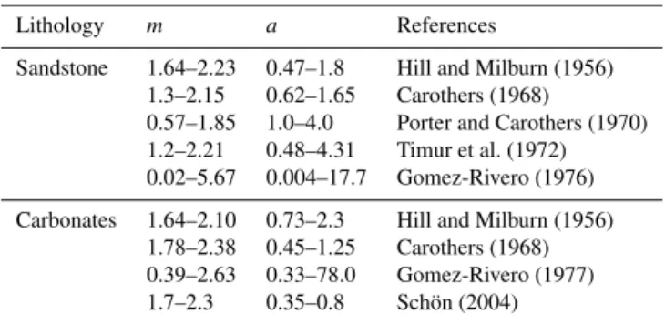
Table 1 shows typical ranges of values for the cementation exponent and theavalue obtained from the literature (Wor-thington, 1993). Clearly thea parameter may vary greatly. However, some of the more extreme values given in the ta-ble are probably affected by artefacts. A quick look at the age of some of these data indicates another problem: while there is a huge amount of existing Archie’s law data, most are proprietorial, and the few datasets that have been pub-lished are relatively old. We have conducted our analyses on recent data. The data are all owned by a single multinational
Table 1.Typical ranges of cementation exponent and thea param-eter from the literature (Worthington, 1993).
Lithology m a References
Sandstone 1.64–2.23 0.47–1.8 Hill and Milburn (1956) 1.3–2.15 0.62–1.65 Carothers (1968)
0.57–1.85 1.0–4.0 Porter and Carothers (1970) 1.2–2.21 0.48–4.31 Timur et al. (1972) 0.02–5.67 0.004–17.7 Gomez-Rivero (1976)
Carbonates 1.64–2.10 0.73–2.3 Hill and Milburn (1956) 1.78–2.38 0.45–1.25 Carothers (1968) 0.39–2.63 0.33–78.0 Gomez-Rivero (1977) 1.7–2.3 0.35–0.8 Schön (2004)
oil company, having commissioned one or more service com-panies to make the actual measurements. The company has been asked to allow us to provide the provenance of the data, but have demanded that their source remains unattributable as a condition of their use due to the sensitivity of some of the measurements. While this is not an ideal situation, it does allow real numerical data to be available in the public domain when they would otherwise remain secret, and it shows the typical quality of data used by the oil industry at present.
In a paper such as this, the dataset is very important. The inferences made at the end of this paper have a bearing on the quality of data measurement. First of all, the dataset should be typical of its type within the oil industry, and prefer-ably represent the best or close to the best practice within the industry. Generally service companies have very well-developed protocols for making the best and most reliable as well as the most repeatable measurements possible within tight financial constraints. Consequently, the data are often of high quality, but not as high as it might be if the measure-ment were carried out in an academic environmeasure-ment with no pressures of time or funding.
of pore fluid salinity and pore fluid conductivity are generally made on the stock solution that is used to saturate the sam-ples. The degree of saturation may not be complete depen-dent upon the method used, and whether vacuum saturation is combined with the addition of a high pressure afterwards. Once again, the same protocol would have been used for all samples. That will lead to a good repeatability, but only if the samples are all other similar porosity. If some samples have a much lower porosity than others, then it is possible for the high porosity samples to be, say, 95 % saturated, while the lower porosity samples may only be 50 % saturated. It is not common for fluids to be flowed through the rock in order for the rock and pore fluids to attain chemical equilibrium. Con-sequently, the real conductivity of the pore fluid will not be the same as that of the stock solution and there is potential for error. This error might be variable, depending upon the degree to which each sample contains matrix material in fine powdery form that might dissolve in the pore fluid more eas-ily. Protocols are usually sufficiently robust to ensure that all measurements are made at the same temperature, or that cor-rections for temperature are put in place. However, there is the potential for human error.
In this work all of the data are from relatively clean clastic reservoirs whose dominant mineralogy is quartz, exhibiting a low degree of surface conduction. However, there is no rea-son why the arguments made in this paper should not apply equally well to carbonates (e.g. Rashid et al., 2015a, b) or in-deed any reservoir rock for which Archie’s parameters might be useful in determining their permeability (e.g. Glover et al., 2006; Walker and Glover, 2010).
2 Model comparison
The question why the practice of using an equation that is not theoretically correct remains commonly applied in in-dustry is worth asking. The answer is that the variant form of Archie’s law (Eq. 2) generally fits the experimental data much better than the original form (Eq. 1).
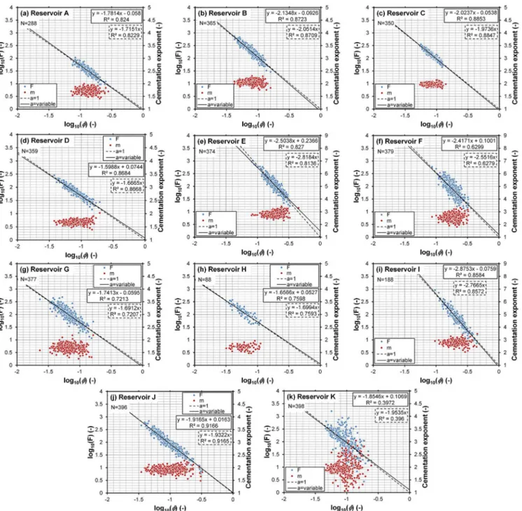
We have carried out analysis of a large dataset using the two equations and by calculating the cementation exponents for individual core plugs. Figure 1 shows formation factors (blue symbols) and cementation exponents (red symbols) of the fully saturated rock sample as a function of porosity for 3562 core plugs drawn from the producing intervals of 11 unattributable clean sandstone and carbonate reservoirs. The formation factor data have been linearised by plotting the data on a log axis against the porosity, also on a log axis. Best fits were made by linear regression from both the Win-sauer et al. (1952) variant of the first Archie’s law (Eq. 2, solid lines) and the theoretically correct first Archie’s law (Eq. 1, dashed lines). In addition, the individually calculated cementation exponents were calculated by inverting Eq. (3) (red symbols).
A first qualitative comparison of the fits in Fig. 1 shows that fitted lines from both equations seem to describe the data very well and it would be tempting to assume that ei-ther would be sufficient to use for reservoir evaluation. The adjustedR2coefficients of the fits of Eqs. (1) and (2) to the data are also shown in Fig. 1 and are also summarised in Table 2. They show that Eq. (2) is a better fit in all cases, with slightly higher adjustedR2coefficients, but the differ-ence is extremely small. One might be tempted to attribute the slightly better fit of Eq. (2) to the fact that it has one more fitting parameter.
There is, however, an important difference in the values of cementation exponent that the two methods of fitting provide. The cementation exponents that are derived from each fit are shown in the regression equations given in each panel of Fig. 1 and are summarised in Table 2. It is clear that there is a significant difference in the cementation exponents derived from the two different equations in almost every case. The extent of the differences is clear in Fig. 2, where the cemen-tation exponents calculated from Eq. (1) and from Eq. (2) are plotted as a function of the mean of the individual exponents calculated using Eq. (3), with the dashed line representing a 1 : 1 relationship. There is no significance in the almost perfect agreement between Eq. (1) and the mean of the in-dividual core plug determinations as both measurements are based on the same underlying equation, that of Archie’s orig-inal law. What is surprising is that the difference between the cementation exponents derived from using Eq. (2) dif-fers significantly from the difference between those that used Eq. (1).
The small, but apparently significant differences in ad-justedR2fitting statistic have prompted us to analyse the fits in greater depth in Fig. 3. In this figure the right-hand ver-tical axis shows the percentage difference between the ad-justedR2 value from fitting Eq. (2) with respect to Eq. (1) as a function of the parameter a from Eq. (2). In all the cases except one, the percentage difference is less than 0.5 %, which is very small. The points do, however fall on a well-fitted quadratic curve that is centred on, and falls to zero at a=1. This shows that the percentage difference between us-ing these two models behaves predictably, and the two mod-els are equivalent ata=1 as expected.
Figure 1.Formation factor and cementation exponent of the fully saturated rock sample as a function of porosity for 3562 core plugs drawn from the producing intervals of 11 clean sandstone and carbonate reservoirs. Blue symbols represent the formation factor for individual core plugs calculated asF=ρo/ρf and red symbols represent cementation exponents for individual core plugs calculated with Eq. (3). The solid
line is the best fit to the Winsauer et al. (1952) variant of the first Archie’s law (Eq. 2), while the dashed line is the best fit to the original first Archie’s law (Eq. 1), each with adjustedR2coefficients.
be very significant differences in the cementation exponents obtained using the two different Archie’s equations.
Consequently, statistical analysis of the 3562 data points analysed in this work shows that Eq. (2) provides a better fit than Eq. (1), confirming the experience of many petrophysi-cists. Equation (2) provides a better physical quality of fit to real data despite the data being theoretically flawed, and
Table 2.Summary data from the 11 test reservoirs.
Application of Eq. (2) Application of Eq. (1) Winsauer et al. (1952) Archie (1942)
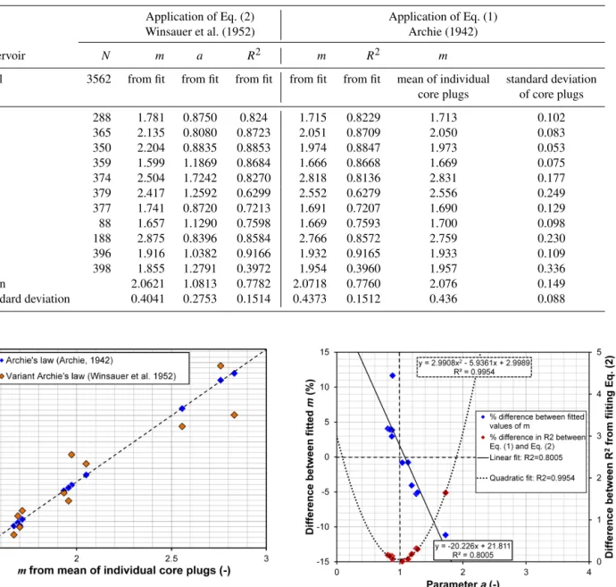
Reservoir N m a R2 m R2 m
Total 3562 from fit from fit from fit from fit from fit mean of individual standard deviation core plugs of core plugs A 288 1.781 0.8750 0.824 1.715 0.8229 1.713 0.102 B 365 2.135 0.8080 0.8723 2.051 0.8709 2.050 0.083 C 350 2.204 0.8835 0.8853 1.974 0.8847 1.973 0.053 D 359 1.599 1.1869 0.8684 1.666 0.8668 1.669 0.075 E 374 2.504 1.7242 0.8270 2.818 0.8136 2.831 0.177 F 379 2.417 1.2592 0.6299 2.552 0.6279 2.556 0.249 G 377 1.741 0.8720 0.7213 1.691 0.7207 1.690 0.129 H 88 1.657 1.1290 0.7598 1.669 0.7593 1.700 0.098 I 188 2.875 0.8396 0.8584 2.766 0.8572 2.759 0.230 J 396 1.916 1.0382 0.9166 1.932 0.9165 1.933 0.109 K 398 1.855 1.2791 0.3972 1.954 0.3960 1.957 0.336 Mean 2.0621 1.0813 0.7782 2.0718 0.7760 2.076 0.149 Standard deviation 0.4041 0.2753 0.1514 0.4373 0.1512 0.436 0.088
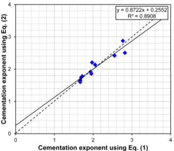
Figure 2. Cementation exponent derived from fitting Archie’s (1942) law (Eq. 1, solid blue symbols) and the Win-sauer et al. (1952) variant of Archie’s law (Eq. 2, solid orange symbols) as a function of the cementation exponent derived as the mean of the cementation exponents calculated from data from individual core plugs using Eq. (3), which is based on Archie’s original law. The dashed line shows a 1 : 1 relationship. Each symbol represents data from one of the 11 reservoirs analysed in Fig. 1.
3 Implications for reserves calculations
We have compared the results of the calculated cementation exponents from each of the equations using the 11 reser-voirs that are summarised in Table 2. The mean cementa-tion exponent from fitting Eq. (2) to the whole dataset is m=2.062±0.404 (one standard deviation), while that from
Figure 3.Percentage difference between cementation exponents derived from Eq. (2) with respect to that derived from the use of Eq. (1) (i.e. mEq. 2−mEq. 1/mEq. 1×100) as a function
of the a parameter (blue symbols), with a linear least-squares regression (R2=0.8005), together with the percentage differ-ence between the adjustedR2 fitting coefficients for fitting with Eq. (2) with respect to that derived from the use of Eq. (1) (i.e.R2Eq. 2−R2Eq. 1/REq. 12 ×100)as a function of thea pa-rameter (red symbols), with a quadratic least-squares regression (R2=0.9954).
be-Figure 4.Cross-plot of the cementation exponents calculated using Eqs. (1) and (2) for a database of 3562 core plugs drawn from the producing intervals of 11 unattributable clean sandstone and car-bonate reservoirs. The solid line shows the least-squares regression and the dashed line shows the 1 : 1 ideal.
tween the two methods that is represented by the scatter on this graph, but which could easily be assumed not to be sys-tematic. It is only when the percentage difference between the two derived cementation exponents is plotted against the parametera, (Fig. 3) that the systematic nature of the differ-ence becomes apparent.
Hence, even though Eq. (2) provides only a marginally better fit than Eq. (1), its application can give cementation exponents that are as much as ±11 % different from those obtained with Eq. (1) for the data from our 11 reservoirs, but may be even larger if the literature values are reliable (Ta-ble 1).
For example, if one assumes arbitrarily that the true ce-mentation exponent ism=2.072, and then accepts that sys-tematic error in the use of Archie’s law is±11 %, the calcula-tion of the stock tank hydrocarbon in place shows an error of +20.13/−16.76 % in reserves calculations. In this last cal-culation we have used typical reservoir values (a saturation exponent,n=2; porosity,φ=0.2; reservoir fluid resistivity in situ, ρφ=1m; effective rock resistivity,ρt =500m). The error in the reserves calculation is independent of the reservoir’s areal extent, its thickness, its mean porosity, or its formation volume factors. This error indicates clearly that the accuracy of our calculations of the cementation exponent should be of prime importance, especially with reservoirs be-coming smaller, more heterogeneous, and more difficult to produce.
In summary, apparent small differences in fit can cause significant differences in the derived cementation exponent which will have important implications for reserves calcula-tions. Moreover, it is the Winsauer et al. (1953) variant of
Archie’s equation which contains the theoretically unjusti-fied a parameter, which seems to produce a better fit than the classical Archie’s law. However, it is not known which approach is better at this stage. The remainder of this paper attempts to find reasons for the disparity between the two equations so that the best approach can be chosen.
Therefore, there is an apparent paradox: Eq. (2) is theo-retically incorrect but fits the data better than a theotheo-retically correct form. There are two possible reasons.
1. The theoretically correct form of the first Archie’s law is wrong.
2. All of the experimental data are incorrect.
Moreover, it is incredibly important to find out the reason for the apparent paradox, given the implications for reserves calculations that we have described above.
Furthermore, Table 1 and our analysis of 11 reservoirs shows that theaparameter can take values both greater than and less than unity, indicating that there may be more than one contributory effect.
4 Error in the formulation of Archie’s law
One of the possibilities for the observed behaviour is that the original Archie’s law is incorrect. If that is the case we can hypothesise that there is an unknown mechanismX oc-curring in the rock which either (i) scales linearly with the pore fluid resistivity, or which (ii) scales with the porosity to the power of the cementation exponent (rather than the neg-ative of the cementation exponent). In other words, an im-proved Archie’s law should look like either of the following two equations:
ρo=Xρfφ−m, or (4)
ρo=ρf Xmφ −m
. (5)
Both of these equations are formally the same as Eq. (2), but are rewritten here in generic form so that they may be compared with equations later in the paper that examine the effects of errors in porosity and fluid salinity. However, we have not identified the linear process thatXcould represent. The process cannot be that of surface conduction mediated by clay minerals because of the following reasons.
1. The effect occurs in clean rocks – Fig. 1 shows it op-erating in 11 reservoirs composed of clean sedimentary rocks.
(Ruffet et al., 1995; Revil and Glover, 1997; Glover et al., 2000; Glover, 2010).
4. It is not possible to generate the second scenario from any of the previous theoretical approaches to electri-cal conduction in rocks (Pride, 1994; Revil and Glover, 1997, 1998).
Finally, it is worth remembering that, although initially an empirical equation, Archie’s first law now has a theoret-ical pedigree since its proof (e.g. Ewing and Hunt, 2006). It seems unlikely, therefore, that the theoretical equation is wrong in itself.
5 Error in the experimental data
It is worth taking a little time to imagine the implications of this question. It implies that the majority or even all of the electrical measurements made in petrophysical laboratories around the world since 1942 have included significant sys-tematic errors (random measurement errors are not the issue here). Given the importance of the calculation of the cemen-tation exponent for reserves calculations, this statement will seem incredible and will have far-reaching implications.
It is hypothesised in this paper that there have been sys-tematic errors in the measurement of the electrical properties that contribute to the first Archie’s law. The result of these errors has been to make the version of the first Archie’s law given in Eq. (2) a better model for the erroneous data than the theoretically correct model (Eq. 1), and implies that the theoretically correct model would be a better fit to accurate experimental data. If correct, it would also imply that most of the cementation exponents that have been calculated his-torically are correct because the errors in the experimental data have been compensated for by the parametera. Hence, despite appearing as an empirical parameter, it would have an incredibly important role in ensuring that the calculated cementation exponent is accurate, even with erroneous perimental data. A further implication is that cementation ex-ponents calculated using individual core plugs or a mean of individual core plug measurements are only accurate if the measurements contained none of the systematic errors that are described below.
There are at least three possible sources of systematic er-ror in the relevant experimental parameters used in Archie’s laws, and others may be realised in time. Each has the po-tential for ensuring that the Winsauer et al. (1952) variant of Archie’s law will fit the data better than the classical Archie’s law. These errors are associated with the measurement of porosity, fluid resistivity, and temperature, and will each be reviewed in the following subsections.
5.1 Porosity
Let us assume that if instead of measuring the correct poros-ityφ, we measure an erroneous porosity given byφ+δφ, we
Figure 5.The calculated value of the parameteraas a function of the percentage error in porosity for various values of cementation exponent (given in the legend). Theaparameter is independent of the actual value of the porosity.
have
ρo=ρfφ−m=aρf(φ+δφ)−m, (6) which allows us to calculate the parametera:
a=
φ φ+δφ
−m
. (7)
It is worth noting that the value ofadepends on the cemen-tation exponent, with Eq. (7) expressed as a function of the fractional systematic error in the porosity measurementNφ:
a=
1 1±Nφ
−m
. (8)
If there is a±10 % systematic error in the measurement of the porosity of a rock, and we takem=2, we can generate values fora=1.21 anda=0.81 for the positive and nega-tive cases, respecnega-tively. Figure 5 shows the same calculation as a function of percentage systematic error in the porosity measurement. It is clear that possible systematic errors can produce values of thea parameter that fall in the observed range.
There are many ways of measuring porosity, and it is well known that they give systematically different results. Without being comprehensive, we should consider at least three types of porosity measurements that are commonly used as inputs to the first Archie’s law for the calculation of the cementation exponent.
Helium porosimetry is well known to give effective porosi-ties that are systematically higher than other methods because the small helium molecules can access pores in which other molecules cannot fit. Hence, it is a good measure of the combined effective micro-, meso-, and macro-porosity of a rock.
Mercury porosimetry Again, this method is well known to give effective porosities that are systematically lower than other methods because it takes extremely high pressures to force the non-wetting mercury into the smallest pores. Consequently, the micro-porosity is not commonly measured, even with instruments which can generate very high pressures.
Saturation porosimetry This method relies on measuring the dry and saturated weights of a sample, and then us-ing either caliper measurements or Archimedes’ method for obtaining the bulk volume, from which the porosity may be calculated. Measurements made in this way gen-erally fall between those made on the same sample us-ing the helium and mercury methods. The problem here is one of saturation. If the sample is not fully saturated, the porosity will be underestimated. Since saturation in any laboratory is generally governed by its protocols, attainment of an only partially saturated sample would be systematic.
There is scope for a study to discover which method for measuring porosity is the best for use with Archie’s law. Such a study, however, would need to remove all other sources of systematic error in order to find the best porosity measure-ment method reliably.
5.2 Pore fluid salinity
It is important to distinguish between (i) the bulk pore fluid resistivity and (ii) the resistivity of the fluid in the pores. The bulk pore fluid resistivity is that fluid which has been made in order to saturate the rock. It has a given pH and resistivity, which may be measured in the laboratory, but is sometimes calculated from charts, using software, or empirical models such as that of Sen and Goode (1992a, b). It is the resistivity of this fluid that petrophysicists have most commonly used in their analysis of data using the first Archie’s law.
However, the first Archie’s law is not interested in the bulk fluid resistivity, but the actual resistivity of the fluids in the pores. When an aqueous pore fluid is flowed through a rock sample, it changes. Precipitation and, more commonly,
dis-solution reactions occur until the pore fluid is in physico-chemical equilibrium with the rock sample.
We have carried out tests on three samples of Boise sand-stone, and we find that the fluid in equilibrium with the rock can have a resistivity up to 100 % less than the bulk fluid (and a pH that is up to±1 pH points different). These sam-ples have a large porosity; quartz content is between 80 and 90 %, feldspar and mica content is between 10 and 20 %, and there is a very little clay fraction. The surface conduction was assessed as being between 13.6 and 32×10−4S m−1 (Walker et al., 2014), which is lower than most of the pe-riod sandstone and Fontainebleau sandstone samples we have recently measured, and consequently the Boise sandstone is considered to be a reasonable analogue for the clay free clas-tic reservoir data used in this work. In these tests a bulk fluid was made by dissolving pure NaCl in deaerated and deioinised water. The fluid was deaerated once again and brought to a standard temperature (25±0.1◦C). The bulk
re-sistivity of the solution was then measured using a benchtop resistivity meter that had been calibrated using a high-quality impedance spectrometer. Two litres of the fluid was placed in a container and pumped through a rock sample that had been saturated with the same fluid, and arranged so that the emerg-ing fluid was returned to the input reservoir and mixed with it. The circulation of fluids was continued until either 1400 pore volumes had been passed through the sample or the re-sistivity of the emerging fluids had reached equilibrium. The resistivity of the emerging fluids was measured with the same resistivity meter in the same way as the bulk fluid and at the same temperature. Further experimental details can be found in Walker et al. (2014). Figure 6 shows the difference be-tween the resistivity of the bulk fluid and the resistivity of the actual pore fluids for a range of fluids with different starting salinities. The figure shows clearly that low resistivity bulk fluids become significantly less resistive as they equilibrated with the rock, and this has been associated with dissolution of rock matrix in the fluid. The effect is sufficiently large at low salinities to preclude the possibility of having a very low-salinity fluid equilibrated with the rock, and can lead to increases in fluid conductivity of up to 100 % if the initial bulk fluid has a conductivity of less than 10−3S m−1. How-ever, the effect is significant, even at greater salinities with bulk fluids with an initial conductivity of 0.1 S m−1 undergo-ing an increase of up to 16 %. There is even the intimation of very high initial salinity bulk solutions decreasing in salin-ity and conductivsalin-ity slightly upon equilibration with the rock sample, an effect that we associate with a slight tendency to precipitate salt within the rock or to react with it.
The apparent clear difference between the resistivity of the bulk fluid, which is used as an input to Archie’s first law, and the resistivity of the fluid, which should be used, is clearly the source of an invisible systematic error to which many petrophysical laboratories have succumbed.
Figure 6. Percentage difference between the conductivity of the fluid in the pores and that of the bulk fluid originally used to sat-urate the rock as a function of the resistivity of the fluid in the pores for three samples of Boise sandstone.
fluid given byρf+δρf, whereδρf will be positive for low-and medium-salinity fluids due to dissolution low-and negative for high-salinity fluids where there may be precipitation. We then have
ρo=ρfφ−m=a ρf +δρf
φ−m, (9)
which allows us to calculate the parameteraas a= ρf
ρf+δρf
(10) or as
a= 1 1±Nρf
, (11)
whereNρf is the fractional systematic error in the fluid re-sistivity measurement.
If there is a +10 % systematic error in ρf, which is the case approximately for a fluid solution of 0.1 mol dm−3 (Fig. 6), we can calculatea=0.91, which is in the range of observed values. Hence the erroneous assumption that the bulk fluid resistivity represents the resistivity of the fluid in the pores can easily produce the observed effect, and much bigger values ofawould be possible if lower bulk fluid salin-ities were used to saturate the rock if it were the resistivity of those fluids that was directly used in the first Archie’s law. 5.3 Temperature
Temperature also affects the pore fluid resistivity that we use in the first Archie’s law. The resistivity of an aqueous pore fluid changes by about 2.3 % per ◦C at low temperatures (< 100◦C). Sen and Goode (1992a, b) provide an extremely useful empirical model for calculating the conductivity of an
Figure 7.Resistivity of an aqueous solution of NaCl as a function of temperature for a number of different pore fluid salinities using the method of Sen and Goode (1992a, b). Dashed lines show the change in conductivity resulting from a difference in temperature between 20 and 25◦C. Note that the normalised curves from the whole range of salinities including in the figure are almost coincident.
aqueous solution of NaCl as a function of temperature and salinity up to 100◦C. This model has been implemented in Fig. 7 for conductivity and for a range of fluid salinities. In this figure we have normalised the curves for each of the salinities to that at 20◦C. This allows us to see that the
rel-ative variation of conductivity for all the pore fluid salinities in the figure are approximately the same, as well as enabling the difference in conductivity with respect to 20◦C to be cal-culated easily.
If we measure the pore fluid resistivity, or calculate it us-ing the model at 25◦C, but measure the resistivity of the sat-urated rock sample at 20◦C (or vice versa), we will introduce a systematic error in the measurements that can be large. Fig-ure 7 shows that the error in such a temperatFig-ure mismatch is approximately the same for all fluid salinities, and would be between−12.03 and 12.34 % depending on the fluid salinity (largest for the highest salinities). Equation (10) can be used to calculate that a value ofa=1.25 would be introduced to the first Archie’s law fitting when using Eq. (2) to calculate the cementation exponent with a bulk rock resistivity mea-surement that is made at a temperature 5◦C lower than that
at which the bulk fluid had been measured. Hence, once again a systematic error of the correct magnitude is obtained from a lack of temperature control.
flu-Figure 8. Modelling of the calculated cementation exponent and
a parameter for error-free data and data containing two types of systematic error in porosity,(a)measured porosity exceeds the real porosity by 0.02, and(b)measured porosity exceeds the real poros-ity by a factor of 1.2. Solid curves and dots refer to the left-hand vertical axis. The orange dashed line refers to the right-hand axis.
ids should both have the same temperature. Providing the pore fluid has been equilibrated properly with the sample, this procedure also removes any errors associated with using the resistivity of unequilibrated bulk fluids in Archie’s law calculations.
6 Discussion
Equations (6) to (11) mathematically imply that the use of the a parameter might be compensating for any systematic errors. This perhaps surprising result is analysed in the fol-lowing section. The implications of errors in porosity will be analysed, though the argument applies equally to errors in
fluid saturation or temperature, and the final result in reality will be a mixture of all three errors.
First, let us assume that we are using Archie’s law to cal-culate the cementation exponent of a single core plug. Equa-tion (1) can be used in its rearranged form (Eq. 3). If we as-sume that the measurements of porosity, fluid resistivity, and core plug resistivity are all accurate, then Eq. (3) will give an accurate value of cementation exponent. Conversely if there is an error in any of the input parameters, they will be in error in the cementation exponent. Equation (2) can also be rearranged for the calculation of cementation exponent, but since there is no a priori knowledge of the value of thea pa-rameter, the calculation cannot be carried out. Consequently, when calculating a single value of cementation exponent for a single core plug, the accuracy of cementation exponents de-pends critically upon the accuracy of the input data, whether the errors are random or systematic.
Now let us examine the calculation of cementation expo-nent from a population of core samples by the fitting of the original or Winsauer et al. variants of Archie’s law. Three possibilities will be analysed, of which the results of two are shown in Fig. 8. The three possibilities are that there is a random error (which is not shown in the figure), a system-atic error resulting in the measured porosity of each sample being overestimated or underestimated by a constant value (Fig. 8a), and a systematic error resulting in the measured porosity of each sample being overestimated or underesti-mated by a constant fraction of the real value (Fig. 8b). Both graphs are given as a function of the real error-free porosity. The figure assumes that the real fluid resistivity is 10m, and the real cementation exponent is 2.1; however, these are generic values, and any value for these parameters could have been taken with the same result. The horizontal green lines in both parts of the figure represent the real cementation ex-ponent,m=2.1. This value has been used to calculate the resistivity of the sample, which varies with porosity. Con-sequently, we take the resistivity of the sample, that of the pore fluid, and the valuem=2.1 to represent the target re-ality. The next step is to use the values of the resistivity of the sample and that of the pore fluid together with the mea-sured porosity in order to calculate the value of the cemen-tation exponent. In Fig. 8a we assume that every instance of measured porosity is overestimated by 0.02 (or two porosity units). That represents a very large fractional error for those samples that really do have a low porosity, and a small frac-tional error for samples with a real porosity approaching 0.3. Using Eq. (1) to calculate the cementation exponent of this error-prone data, we obtain the blue curve in Fig. 8a, which varies from m=3.02 at low porosities (x axis=0.005) to m=0.32 at high porosities (x axis=0.3). Clearly, the con-stant over- or underestimation of porosity, by a small amount, has a large effect upon the calculated cementation exponent if Eq. (1) is used.
population. In this example we have used Eq. (7). The only practical difference between these two approaches is that this demonstration explicitly calculates thea parameter for each point on the curve, whereas in practice theaparameter would represent some means of those for each of the samples in the population. In Fig. 8a the dashed orange line, which uses the right-hand vertical axis, shows that the a parameter varies widely, from very high values approaching 30 at low ties, to much lower values approaching 1.14 at high porosi-ties, for these particular input parameters. Implementation of Eq. (2) with the error-prone porosity data now gives the dot-ted curve in the figure. The calculadot-ted value of cementation exponent is in all cases m=2.1, and thea value has auto-matically “compensated” for the error in the porosity.
Figure 8b shows that exactly the same process was im-plemented for a systematic error which is a constant mul-tiple of the real porosity, which in this example is a factor of 1.2, but could be much higher than unity or much less than unity with the same general effect. Once again the use of Eq. (1) with the error-prone data provides an erroneous calculated cementation exponent varying betweenm=2.1 at low porosities andm=2.47 at high porosities. For the case of a systematic error which is a constant multiple of the real porosity thea value is constant, in this case a=1.466. Its use in Eq. (2) once again provides the accurate cementation exponent across the whole porosity range, as shown by the dots in Fig. 8b. Thea parameter has again compensated for the systematic errors in the porosity.
Similar analyses can be done with the fluid resistivity vari-able and as a function of temperature, with exactly the same results. The individual changes in thea parameter compen-sates for the error in the variable. Since all the equations are linear, then any mixture of systematic errors will lead to a lin-ear mixing of their individual consequent a values, taking au-tomatic account of errors which balance each other to some extent. Consequently, it is not necessary to know in which of the three parameters systematic errors occur, or even to know the extent to which there is an error in each of the pa-rameters. The resultinga parameter takes it all into account automatically. The size of the a parameter is an indication of the extent to which there is an overall systematic error in the measurements, but it does not tell you in which of the pa-rameters the systematic error or errors reside, or whether any of the three parameters are more accurate than the others, or indeed whether systematic errors in two or more parameters compensate to some extent for systematic error in the third. The a parameter can therefore be considered as a quantita-tive measure of the overall accuracy of the parameters used to calculate cementation exponent.
The remaining error type to consider is random error. However, these errors are automatically removed from any fitting that is carried out using either equation by the least-squares operation, and so are not considered further in this work.
In summary, examination of the sources of error described above allows us to make the following two statements. The first is that if Eq. (2) has been used, the systematic measure-ment errors do not affect the calculated value of the cemeasure-menta- cementa-tion exponent because the fitted value of theaparameter has compensated for the presence of the errors. In other words, the cementation exponents that petrophysics have been cal-culating with Eq. (2) and using erroneous data are, and have always been correct, providentially. They are the same ce-mentation exponents that we would have calculated if we had applied the theoretically correct first Archie’s law (Eq. 1) to error-free data. The second is that if Eq. (1) has been used ei-ther by fitting to a group of data or by individual calculation of cementation exponents, the cementation exponents will be in error, possibly significantly, unless the experimental data that have been used are free from all sources of systematic error.
It is possible to make recommendations for the improve-ment of the accuracy of data used in the first Archie’s law, as follows.
1. The saturation of samples should be as close to 100 % as possible. Vacuum and pressure saturation followed by flow under back-pressure can be recommended. Full saturation can be improved by flooding the sample with CO2prior to saturation. It is also beneficial to degas the saturating fluids using a vacuum or reverse osmosis, or by bubbling helium through the saturating fluid. 2. There is some ambiguity about what is the “correct”
porosity to use with the first Archie’s law. Until this is resolved, it is recommended in this paper that the poros-ity calculated from the saturation of the sample with the reservoir water by dry and saturated weights is carried out, and Archimedes’ method is used to measure the bulk volume of the core plug. Other sources of poros-ity should be avoided.
3. The resistivity of both the bulk fluid and the fluid in equilibrium with the rock sample should be measured, with the latter being used in the first Archie’s law to cal-culate the cementation exponent. This implies that fluid is flowed through the core until equilibrium is attained. This process may take several days.
4. All measurements of bulk fluid resistivity, equilibrium resistivity, and effective resistivity of the saturated rock sample should be either made at the same temperature, or all corrected to a standard temperature.
7 Conclusions
This paper shows that the commonly applied Winsauer et al. (1952) variant of the first Archie’s law is incorrect the-oretically, yet paradoxically fits data better than the classical, and formally correct, Archie’s law.
The apparent paradox can be explained by systematic er-rors in the majority of all previous data. Erer-rors in porosity, pore fluid salinity, and temperature can all explain the effect and may combine to produce the observed results.
Consequently, cementation exponents which have been calculated historically using the Winsauer et al. (1952) vari-ant of the first Archie’s law (Eq. 2) will be accurate be-cause theaparameter has compensated for whatever system-atic experimental errors exist in the data. Nevertheless, ce-mentation exponents calculated using the classical Archie’s law (Eq. 1) or on individual core plugs using (Eq. 3), i.e. m= −logF /logφ, probably do contain significant errors.
A range of recommendations have been made to improve the accuracy of calculations of the cementation exponent us-ing the first Archie’s law. Furthermore, the parametera can be used as a new data quality parameter, where values ap-proachinga=1 indicate high-quality data.
8 Data availability
While the raw data used in this work remain confidential, the summary and generic data that are shown in the figures have been provided as a Supplement to this publication.
The Supplement related to this article is available online at doi:10.5194/se-7-1157-2016-supplement.
Edited by: D. B. Dingwell
Reviewed by: H. Milsch and one anonymous referee
References
Archie, G. E.: The electrical resistivity log as an aid in determining some reservoir characteristics, Trans. AIME, 146, 54–67, 1942. Carothers, J. E.: A statistical study of the formation factor relation,
Log Anal., 9, 13–20, 1968.
Ewing, R. P. and Hunt A. G.: Dependence of the electrical con-ductivity on saturation in real Porous media, Vadose Zone J., 5, 731–741, doi:10.2136/vzj2005.0107, 2006.
Glover, P. W. J.: What is the cementation exponent? A new inter-pretation, The Leading Edge, 28, 82–85, doi:10.1190/1.3064150, 2009.
Glover, P. W. J.: A generalised Archie’s law for nphases, Geo-physics, 75, E247–E265, doi:10.1190/1.3509781, 2010. Glover, P. W. J.: Geophysical properties of the near surface Earth:
Electrical properties, Treatise on Geophysics, 11, 89–137, 2015.
Glover, P. W. J., Hole, M. J., and Pous, J.: A modified Archie’s Law for two conducting phases, Earth Planet. Sc. Lett., 180, 369–383, doi:10.1016/S0012-821X(00)00168-0, 2000.
Glover, P. W. J., Zadjali, I. I., and Frew, K. A.: Permeability predic-tion from MICP and NMR data using an electrokinetic approach, Geophysics, 71, F49–F60, doi:10.1190/1.2216930, 2006. Gomez-Rivero, O.: Some considerations about the possible use of
the parameters a and m as a formation evaluation tool through well logs, Trans. SPWLA 18th Ann. Logging Symp., J1–24, 1977.
Hill, H. J. and Milburn, J. D.: Effect of clay and water salinity on electrochemical behaviour of reservoir rocks, Trans. AIME, 207, 65–72, 1956.
Porter, C. R. and Carothers, J. E.: Formation factor porosity relation derived from well log data, Trans. SPWLA 11th Ann. Logging Symp., 1–19, 1970.
Pride, S.: Governing equations for the coupled electromagnetics and acoustics of porous media, Phys. Rev. B, 50, 15678–15696, doi:10.1103/PhysRevB.50.15678, 1994.
Rashid, F., Glover, P. W. J., Lorinczi, P., Collier, R., and Lawrence, J.: Porosity and permeability of tight carbonate reservoir rocks in the north of Iraq, J. Petrol. Sci. Eng., 133, 147–161, doi:10.1016/j.petrol.2015.05.009, 2015a.
Rashid, F., Glover, P. W. J., Lorinczi, P., Hussein, D., Collier, R., and Lawrence, J.: Permeability prediction in tight carbonate rocks using capillary pressure measurements, Mar. Petrol. Geol., 68, 536–550, doi:10.1016/j.marpetgeo.2015.10.005, 2015b. Revil, A. and Glover, P. W. J.: Theory of ionic surface electrical
conduction in porous media, Phys. Rev. B, 55, 1757–1773, 1997. Revil, A. and Glover, P. W. J.: Nature of surface electrical con-ductivity in natural sands, sandstones, and clays, Geophys. Res. Lett., 25, 691–694, 1998.
Ruffet, C., Darot, M., and Guéguen, Y.: Surface conduc-tivity in rocks: A review, Surv. Geophys., 16, 83–105, doi:10.1007/BF00682714, 1995.
Schön, J. H.: Physical Properties of Rocks: Fundamentals and Prin-ciples of Petrophysics, edited by: Helbig, K. and Treitel, S., vol. 18, Amsterdam, the Netherlands: Elsevier, ISBN: 008044346X, 2004.
Sen, P. and Goode, P.: Influence of temperature on electri-cal conductivity on shaly sands, Geophysics, 57, 89–96, doi:10.1190/1.1443191, 1992a.
Sen, P. and Goode, P.: Errata, to “Influence of temperature on electrical conductivity of shaly sands”: Geophysics, 57, 1658, doi:10.1190/1.1443191, 1992b.
Timur, A., Hemkins, W. B., and Worthington, A. E.: Porosity and pressure dependence of formation resistivity factor for sand-stones, Trans. CWLS 4th Formation Evaluation Symp., 30 pp., 1972.
Walker, E. and Glover, P. W. J.: Permeability models of porous media: Characteristic length scales, scaling constants and time-dependent electrokinetic coupling, Geophysics, 75, E235–E246, doi:10.1190/1.3506561, 2010.
Winsauer, W. O., Shearin, H. M., Masson, P. H., and Williams, M.: Resistivity of brine-saturated sands in relation to pore geometry, AAPG Bull., 36, 253–277, 1952.