Functional Equations and Integral Equations in Spectral Domain for Scattering by Impedance Polygons

Functional Equations and Integral Equations in

Spectral Domain for Scattering by Impedance

Polygons

J.M.L. Bernard

Abstract_{—Some features of functional and integral equations} involved in the spectral approach developed by the author (in Qu. J. of Mech. and Appl. Math., 59, 4, pp.517-550, 2006) for scattering by two-dimensional polygonal objects with ar-bitrary surface impedance conditions are presented. In this problem, the Wiener-Hopf method cannot be applied, while asymptotic methods can only be used if corners are widely spaced compared to wavelength, and the presence of imperfectly reflective surfaces particularly complicates the problem. After presenting our method to handle in a global manner the problem of n-part polygonal objects using the Sommerfeld-Maliuzhinets representation of the field, we detail the functional equations for the spectral functions, and the way to reduce them to a system of integral equations of the second kind with non-singular kernels, allowing approximations. We apply in particular this approach to the important class of three-part impedance polygons composed of a finite segment attached to two semi-infinite planes.

Index Terms_{—spectral method, integral equations, functional} equations, helmholtz equation, polygonal surface.

I. INTRODUCTION

S

OME features of functional and integral equations in-volved in the spectral approach developed by the author in [5] for scattering by two-dimensional polygonal objects with impedance boundary conditions are presented. In this delicate exterior problem, the Wiener-Hopf method cannot be applied [1-2], while asymptotic methods can only be used if corners are widely spaced compared to wavelength [3], and the presence of imperfectly reflective surfaces particularly complicates the problem.

To handle the problem, we consider the Sommerfeld-Maliuzhinets representation of the field,

u(ρ, ϕ) = 1 2πi

γ

f(α+ϕ)eikρcosαdα, (1)

which satisfies the Helmholtz equation(∆ +k2_{)u(ρ, ϕ) = 0,}

in free space sector−Φ≤ϕ≤Φwhich contains the scatterer. In this representation, f is an analytic function and the pathγ consists of two branches: one, namedγ+, going from

(i∞+arg(ik) + (a1+π₂))to(i∞+arg(ik)−(a2+π₂))with

0< a1,2 < π, as Imα≥d, above all the singularities of the

integrand, and the other, namedγ−, obtained by inversion of

γ+ with respect toα= 0.

J.M.L. Bernard is with D´epartement de Physique Th´eorique et Appliqu´ee, CEA/DIF-Bruy`eres le Chˆatel, 91297 Arpajon cedex, and, with LRC MESO, CMLA-CEA, 61 av. du Pres. Wilson, 94235 Cachan, France e-mail: [email protected]

Fig. 1. geometry

Fig. 2. coordinates and complex path

This representation has long been devoted to the rigorous analysis of isolated wedges. However, some of our recent developments permit us to consider a new integral expres-sion of the spectral function, in some domain of complex angles, where it becomes possible to take globally account of boundary conditions on a complex geometry [4],[5]. The problem can be then reduced to original difference and integral equations that are studied.

II. SINGLE-FACE EXPRESSION OFf AND ITS USE FOR POLYGONAL OBJECTS

An expression allows to consider arbitrary shapes. For this, we show first [4-5] that

f(±π+ϕ) = 1 2

∞

0

(iku(ρ′_{,±Φ) sin(ϕ∓Φ)}

±∂u

∂n(ρ

′_,±Φ))eikρ′_cos(ϕ∓Φ)

dρ′, (2) as π₂ <Φ∓ϕ◦ < 3₂π and π₂ <Φ∓ϕ < 3₂π, |arg(ik)|<

π

2, whereϕ◦ is the incident plane wave direction, with some

general properties of the field permitting the convergence. Proceedings of the World Congress on Engineering 2008 Vol II

WCE 2008, July 2 - 4, 2008, London, U.K.

Using Green’s theorem, we then note that the contour of integration along ϕ = ±Φ can be deformed into any path L±0,∞, provided that the integral remains bounded and no

source passes through the path during the deformation. So, if we divide the semi-infinite paths L±0,∞ (deriving from a

deformation of the faces ϕ = ±Φ enclosing the scatterer, described above) into L±_0,∆± (i.e. 0 < l′ < ∆±) and L±_∆,∞

(i.e.l′_>∆±_{), we have}

f(±π+ϕ) = 1 2

L± 0,∆±

(ikusin(ϕ−ϕ′

t)± ∂u ∂n)

×eikρ′cos(ϕ−ϕ′)dl′(ρ′, ϕ′) +f_L±

∆±,∞

(±π+ϕ), (3)

wheref_L±

∆±,∞

(α) =e−ikρ_∆±cos(α−ϕ∆±)_f±

e (α),fe±(α)is the spectral function related to the Sommerfeld-Maliuzhinets rep-resentation of the field in coordinates with origin atl′_{= ∆}±_.

We can then write, by analytic continuation, f(α) =1

2

L± 0,∆±

(−ikusin(α−ϕ′t)± ∂u ∂n)

×e−ikρ′_cos(α

−ϕ′₎

dl′_(ρ′_{, ϕ}′_{) +f}

L± ∆±,∞

(α), (4) that is called henceforth the single-face expressions off. Let us consider a polygonal surface located inside the do-main|ϕ|>Φenclosing a scatterer. This surface is composed of two joined semi-infinite polygonal faces, denoted + and

−, respectively withm± _{segments of lengthsd}±

j with tangent angles ±Φ±j,j = 1,2, ..., m± and a semi-infinite plane with tangent angles±Φ±

e. Then, the single face expression of the spectral functionf becomes [5]

f(α) = 1 2

1≤j≤m±

e−ik

1≤i<jd

±

i cos(α∓Φ

±

i)

d±_j

0

(−iku(ρ′

j,±Φ±j) sin(α∓Φ±j)

±∂u

∂n(ρ

′

j,±Φ±j))e− ikρ′

jcos(α∓Φ

±

j)_)dρ′ j

+e−ik

1≤i≤m±d ±

i cos(α∓Φ

±

i)_f±

e,m±(α), (5)

wheref_e,m± ±(α)is the analytic continuation of the integral

expression

f_e,m± ±(α′±Φ±_e) =

1 2

∞

0

(−iku(ρ′e,±Φ±e) sinα′

±∂u

∂n(ρ

′

e,±Φ±e))e−ikρ

′

ecosα

′

dρ′

e, (6) valid as Re(ik(cosα′ _−cos(Φ±

e ∓ϕ◦))) > 0, |Reα′| <

π,|arg(ik)|< π₂.

This original expression of the spectral function and its properties enable us to derive, for the first time, the functional equations for the spectral functions for scattering by a general impedance polygon with finite or infinite surface [5], and to reduce generally the problem to a system of integral equations of the second kind with non-singular kernels.

We apply in particular this approach to the important class of three-part impedance polygons composed of a finite segment attached to two semi-infinite planes.

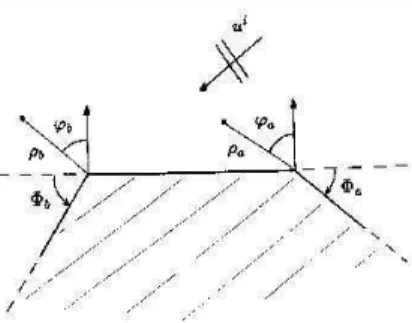
Fig. 3. geometry of three-part impedance polygons

III. FUNCTIONAL ANDINTEGRAL EQUATIONS FOR A SEMI-INFINITE THREE-PART IMPEDANCE POLYGON

The functionsfaandfbare the spectral functions associated with the Sommerfeld-Maliuzhinets representation of the field, in cylindrical coordinate systems (ρa, ϕa) and(ρb, ϕb), with origins at opposite ends of the finite segment. We have, in

(ρa, ϕa)coordinates,

(ρa∈]0,∞[, ϕa=−π₂ −Φa) with ∂u_∂n−iksinθ−u= 0, (ρa ∈[0,∆], ϕa= π₂) with ∂u_∂n−iksinθ1u= 0, (7)

with the incident field ui _=eikρacos(ϕa−ϕ◦)_{, and, in}

coordi-nates(ρb, ϕb),

(ρb∈[0,∆], ϕb=−π₂) with ∂u_∂n −iksinθ1u= 0,

(ρb∈]0,∞[, ϕb= π₂ + Φb) with _∂n∂u−iksinθ+u= 0,(8)

with the incident field ui_=eik(ρbcos(ϕb−ϕ◦)+∆ sinϕ◦)_.

IV. FUNCTIONAL EQUATIONS FOR THE SPECTRAL FUNCTIONS

Functional difference equations for fa andfb are obtained from (5)-(6) with (7)-(8), using parity of some expressions [5]. So, denotingfbr(α−Φ₂b) =fb(α)etΦ+=π₂+Φ₂b, we have

(sinα+ sinθ+)fbr(α+ Φ+)−

−(−sinα+ sinθ+)fbr(−α+ Φ+) = 0,

(sinα−sinθ1)fbr(α−Φ+)−

−(−sinα−sinθ1)fbr(−α−Φ+) =

=e−ik∆ cosα_{((sinα−sinθ}

1)fa(α− π

2)−

−(−sinα−sinθ1)fa(−α−π

2)) =R −

b(α), (9) while, denotingfar(α+Φ₂a) =fa(α)andΦ− =π₂+Φ₂a, we

obtain

(sinα+ sinθ1)far(α+ Φ−)−

−(−sinα+ sinθ1)far(−α+ Φ−) = =e−ik∆ cosα_{((sinα+ sinθ}

1)fb(α+ π

2)−

−(−sinα+ sinθ1)fb(−α+π

2)) =R

+

a(α),

(sinα−sinθ−)far(α−Φ−)

−(−sinα−sinθ−)far(−α−Φ−) = 0. (10)

Proceedings of the World Congress on Engineering 2008 Vol II WCE 2008, July 2 - 4, 2008, London, U.K.

A. Derivation of integral expressions and equations

From functional theory equations, the analytic function χ(α)verifying

χ(α±Φ)−χ(−α±Φ) =ϑ±_{(α), (11)}

and regular in the band|Reα| ≤Φ(even at infinity), is given as |Reα|<Φ, by

χ(α) = χ(i∞) +χ(−i∞)

2 +

−i

8Φ

+i∞

−i∞

(ϑ+(α′_)×

×tan(ν(α+ Φ−α′_))−ϑ−_(α′_{) tan(ν(α−Φ−α}′_)))dα′ ₍₁₂₎

with ν = π

4Φ, when the ϑ

±_{(α) are regular and summable}

on imaginary axis. We then use the solutions Ψ+1(α) (resp.

Ψ1−(α)), without pole or zero in the band|Reα| ≤Φ+ (resp. |Reα| ≤Φ−) andO(cos(πα/2Φ+))(resp.O(cos(πα/2Φ−)))

in this domain, of previous functional equations taken without second member.

We then obtain for −π/2 < ϕ◦ < π/2 + Φb and

−Φ+<Reα <3Φ+,

fbr(α)

Ψ+1(α)

−χib(α) =

= i 8Φ+

+i∞

−i∞

R−

b(α′) tan(4Φπ+(α−Φ+−α ′₎₎

(sinα′_−sinθ

1)Ψ+1(α′−Φ+)

dα′

= −i 4Φ+

+i∞

−i∞

far(α′−π/2 + Φa/2)

Ψ+1(α′−Φ+) ×

× e

−ik∆ cosα′_sin(πα′

2Φ+)

cos(_2Φπ₊(α−Φ+)) + cos(πα

′

2Φ+)

dα′, (13)

where the source termχi

b(α)is given by eik∆ sinϕ◦_χi

+1(α) = 2Φπ+(

eik∆ sinϕ◦_cosπϕ◦,b

2Φ+

Ψ+1(ϕ◦,b)(sin_2Φ+πα −sin πϕ_◦,b

2Φ+ )

), and, for−π/2−Φb< ϕ◦< π/2 et−3Φ−<Reα <Φ−,

far(α)

Ψ1−(α)

−χia(α) =

= −i 8Φ−

+i∞

−i∞

R+

a(α′) tan(4Φπ−(α+ Φ−−α

′₎₎

(sinα′_{+ sinθ}

1)Ψ1−(α′+ Φ−)

dα′

= i 4Φ−

+i∞

−i∞

fbr(α′+π/2−Φb/2)

Ψ1−(α′+ Φ−)

×

× e

−ik∆ cosα′_sin(πα′

2Φ−)

cos(_2Φπ₋(α+ Φ−)) + cos(πα

′

2Φ−)

dα′, (14)

where χi

a(α) = 2Φπ−(

cosπϕ◦,a

2Φ+

Ψ1−(ϕ◦,a)(sin_2Φπα

−−sin

πϕ◦,a

2Φ− )

), with ϕ◦,a=ϕ◦+ Φa/2etϕ◦,b=ϕ◦−Φb/2.

Integral equations for fbr(α+π/2−Φb/2) and far(α− π/2 + Φa/2)can be then derived.

B. non singular integral equations whenΦa,b>−π/2 WhenΦa,b>−π/2, we have, from previous expressions,

fbr(α+π/2−Φb/2)

Ψ+1(α+π/2−Φb/2) −χ i

br(α+π/2−Φb/2) =

= −i 4Φ+

+i∞

−i∞

(far(α

′_{−π/2 + Φ}

a/2)

Ψ+1(α′−Φ+) )

× e

−ik∆ cosα′

sin(πα′

2Φ+)

cos(_2Φπ₊(α−Φb)) + cos(πα

′

2Φ+)

dα′_{, (15)}

as −Φ+<Re(α+π/2−Φb/2)<3Φ+, and,

far(α−π/2 + Φa/2)

Ψ1−(α−π/2 + Φa/2)

−χiar(α−π/2 + Φa/2) =

= i 4Φ−

+i∞

−i∞ (fbr(α

′_+π/2−Φ

b/2)

Ψ1−(α′+ Φ−) )

× e

−ik∆ cosα′_sin(πα′

2Φ−)

cos(_2Φπ₋(α+ Φa)) + cos(πα

′

2Φ−)

dα′, (16)

as −3Φ− <Re(α − π/2 + Φa/2) < Φ−, for −π/2 <

ϕ◦ < π/2. The equations can be solved numerically, or

analytically by approximations, since the term depending on k∆is simple and the source terms are not oscillating. Suitable for approximations whenk∆ is large, we can also transform them by semi-inversion for approximations whenk∆is small.

V. ASEMI-INVERSION TO OBTAIN INTEGRAL EQUATIONS WITH KERNELS VANISHING ASk∆→0

We can modify equations and derive integral equations with kernels vanishing as k∆ →0 for the three-part semi-infinite impedance polygon, for approximations whenk∆is small. For this, we begin with changing the unknowns in the equations (15)-(16), considering far0(α) = far(α)−f0(α−(Φ+ −

π

2), ϕ◦), fbr0(α) =fbr(α)−eik∆ sinϕ◦f0(α+ (Φ−−π2), ϕ◦)

wheref0(α, ϕ◦), corresponding to the solution for∆ = 0, is

known [5]. These functions vanish as∆ = 0, and satisfy, from (15)-(16),

fbr0(α+π2− Φ_b

2 )

Ψ+1(α+π2− Φ_b

2 )

= −i

4Φ+(

+i∞ −i∞(

far0(α′−π2+ Φa

2 )

Ψ+1(α′−Φ+) )

× sin(

πα′

2Φ+)

cos( π

2Φ+(α−Φb))+cos(πα

′

2Φ+) dα′₊

+₋+_ii_∞∞ Ba0(α

′

) sin(πα′

2Φ+)

cos( π

2Φ+(α−Φb))+cos(πα

′

2Φ+)

dα′_{) (17)}

where

Ba0(α′) = (

far0(α′−π2+ Φa

2 )

Ψ+1(α′−Φ+) )(e

−ik∆ cosα′

−1) +

+(e

ik∆ sinϕ◦_f0(α′

−π

2+(Φa−Φb)/2)

Ψ+1(α′−Φ+) )(e

−ik∆(cosα′+sinϕ◦)_−1)(18)

as −Φ+<Re(α+π₂ −Φ₂b)<3Φ+, and

far0(α−π₂+Φ₂a)

Ψ1−(α−π2+ Φa

2 )

=_4Φi₋(₋+_ii_∞∞(fbr0(α′+π2− Φ_b

2 )

Ψ1−(α′+Φ−) )

× sin(

πα′

2Φ−)

cos( π

2Φ−(α+Φa))+cos(

πα′

2Φ−)

dα′₊

+₋+_ii_∞∞ Bb0(α

′_{) sin(}πα′

2Φ−)

cos( π

2Φ₋(α+Φa))+cos(_2Φπα′

−)

dα′_{) (19)}

Proceedings of the World Congress on Engineering 2008 Vol II WCE 2008, July 2 - 4, 2008, London, U.K.

where

Bb0(α′) = (fbr0(α

′

+π

2− Φ_b

2 )

Ψ1−(α′+Φ−) )(e

−ik∆ cosα′_{−1) +}

+(f0(α′+π2−(Φb−Φa)/2)

Ψ1−(α′+Φ−) )(e

−ik∆(cosα′_−sinϕ

◦)_{−1) (20)}

as−3Φ−<Re(α−π₂+Φ₂a)<Φ−, for−min(π₂,π₂+ Φa)< ϕ◦<min(π₂, π₂+ Φb).

We then notice some similarity with the equations satisfied byf0 when ∆ = 0. Thus, we let

f′

br0(α+

π

2 − Φb

2 ) =

=₋i∞_i∞G(ϕ′_)f

0(α+π2 + (Φa−Φb)/2, ϕ′)dϕ′, f′

ar0(α−π2 + Φa

2 ) =

=₋i∞_i∞G(ϕ′_)f

0(α−π₂ + (Φa−Φb)/2, ϕ′)dϕ′ (21) as |Re(α)| < π

2, and search to define G(ϕ′) so that fbr′ 0

andf′

ar0 verifies (17)-(19). The functions f0(α±π₂ + (Φa−

Φb)/2, ϕ′)are regular andO(1/cos(πϕ′/2Φd))on the imag-inary axis, and a pole at ϕ′ _{= α±} π

2 ensures that, even if

Φa= Φb= 0, generallyfbr′ 0=far′ 0.

Using the equations (15)-(16) when∆ = 0satisfied by f0,

we remark that we can write f′

br0(α+π2− Φb

2)

Ψ+1(α+π2− Φ_b

2 )

=

= −i

4Φ+

+i∞ −i∞

far′ 0(α

′

−π

2+ Φa

2 ) sin(πα

′

2Φ+)

Ψ+1(α′−Φ+)(cos(_2Φ+π (α−Φb))+cos(πα

′

2Φ+)) dα′

+_2Φπ₊₋i∞_i∞ G(ϕ′)

Ψ+1(ϕ′− Φ_b

2 )

sinπ(ϕ

′₊π

2) 2Φ+

(cosπ(α−Φb) 2Φ+ +cos

π(ϕ′+π₂) 2Φ+ )

dϕ′_,(22)

f′

ar0(α−π2+ Φa

2 )

Ψ1−(α−π₂+Φ₂a)

= _4Φi₋₋+_ii_∞∞ f

′

br0(α′+π2− Φ_b

2 ) sin(

πα′

2Φ−)

Ψ1−(α′+Φ−)(cos(_2Φπ

−(α+Φa))+cos(

πα′

2Φ−))

dα′

+_2Φπ_{− −}i∞_i∞Ψ G(ϕ′)

1−(ϕ′+Φ2a)

sinπ(ϕ′ −

π

2) 2Φ−

(cosπ(α+Φa) 2Φ− +cos

π(ϕ′ −π

2) 2Φ− )

dϕ′_.(23)

In the case whereG(ϕ′_{)is regular in the band|Re(ϕ}′_{)| ≤}

π

2, we can shift the integral paths in the integrals containing

G(ϕ′_{). Comparing (17)-(19) with (22)-(23), we notice that} (f′

br0, far′ 0)is a solution of the system of equations (17)-(19)

ifGsatisfies the conditions G(α′₊π

2)

Ψ1−(α′+ Φ−)

− G(−α

′₊π

2)

Ψ1−(−α′+ Φ−) =

= i

2π(Bb0(α

′_)−B

b0(−α′)),

G(α′₋π

2)

Ψ+1(α′−Φ+)

− G(−α

′₋π

2)

Ψ+1(−α′−Φ+)

=

=−i 2π(Ba0(α

′_)−B

a0(−α′)), (24)

whereΦ+= π₂+Φ₂b andΦ−= π₂+Φ₂a. Taking account of the

properites of Ψ+1 andΨ1− , and letting G(α′) = (cosα′+

sinθ1)g(α′), (24) can be written

g(α′₊π

2)−g(−α ′₊π

2) =

= iΨ1−(α ′_{+ Φ}

−)(Bb0(α′)−Bb0(−α′))

2π(−sinα′_{+ sinθ}

1) ,

g(α′−π

2)−g(−α ′₋π

2) =

= iΨ+1(α ′_−Φ

+)(Ba0(α′)−Ba0(−α′))

2π(−sinα′_−sinθ

1)

.(25)

Since G(α′_{) is regular in the band |Reα}′_{| ≤} π

2 and

Re(sinθ1) > 0, g(α′) is regular in this band. We can then

use (11)-(12), and write, as|Reα|<π₂, g(α) = i

4π

+i∞ −i∞(

iΨ1−(α′+Φ−)(Bb0(α′)−Bb0(−α′))

2π(sinα′_−sinθ

1) ×

×tan(1₂(α+π₂ −α′₎₎₋iΨ+1(α′−Φ+)(Ba0(α′)−Ba0(−α′))

2π(sinα′_+sinθ

1) ×

×tan(1₂(α−π₂−α′_)))dα′_{, (26)}

Using (21) and (26), we obtain the equations with kernels vanishing as k∆→0 :

fbr0(α+π₂ −Φ₂b) =

= 1 8π2

+i∞ −i∞ dα′(

Ψ1−(α′+Φ−)(Bb0(α′)−Bb0(−α′))

sinα′_−sinθ

1 M+(α, α

′₎

−Ψ+1(α′−Φ+)(Ba0(α′)−Ba0(−α′))

sinα′_+sinθ

1 M−(α, α

′_{)), (27)}

far0(α−π₂ +Φ₂a) =

= 1 8π2

+i∞ −i∞(

Ψ1−(α′+Φ−)(Bb0(α′)−Bb0(−α′))

sinα′_−sinθ

1 N+(α, α

′₎

−Ψ+1(α′−Φ+)(Ba0(α′)−Ba0(−α′))

sinα′_+sinθ

1 N−(α, α

′_))dα′_{, (28)}

whereM±(α, α′) =L±(α+π₂ +(Φa−₂Φb), α′), N±(α, α′) =

L±(α−π2+

(Φa−Φb)

2 , α′),

L±(α, α′) = πsinα

′_Ψ

+−(α)

2Φd

i∞ −i∞

cos(π(ϕ′+(Φa−Φb)/2) 2Φd )

Ψ+−(ϕ′+(Φa−Φb)/2)

(cosϕ′+sinθ1)

cos(ϕ′_±π

2)+cosα′

1 (sin(πα

2Φ_d)−sin(

π(ϕ′+(Φa−Φb)/2) 2Φd ))

dϕ′_{, (29)}

In the particular caseΦa = Φb= 0,Φd= π₂, the functions L±can be simplified so that we recover the expressions found

in [4] for the three-part impedance plane.

REFERENCES

[1] D.S. Jones,The theory of electromagnetism, Pergamon Press, London, 1964.

[2] L.B. Felsen, N. Marcuvitz,Radiation and scattering of waves, Prentice Hall, Englewood Cliffs, NJ, 1973.

[3] V.A. Borovikov, “two-dimensional problem of diffraction on a polygon”,

Sov. Ph. Dokl., 7, 6, 499-501, 1962.

[4] J.M.L. Bernard, “Scattering by a three-part impedance plane : a new spectral approach”,Quarterly J. of Mech. and Appl. Math., 58, 3, pp. 383-418, 2005.

[5] J.M.L. Bernard, “A spectral approach for scattering by impedance polygons”,Quarterly J. of Mech. and Appl. Math., 59, 4, pp.517-550, 2006.

Proceedings of the World Congress on Engineering 2008 Vol II WCE 2008, July 2 - 4, 2008, London, U.K.