Evaluating scale and roughness effects in urban flood modelling using terrestrial LIDAR data

(1)

HESSD

10, 5903–5942, 2013

Evaluating scale and roughness effects in

urban flood modelling

H. Ozdemir et al.

Title Page

Abstract Introduction

Conclusions References

Tables Figures

◭ ◮

Back Close

Full Screen / Esc

Printer-friendly Version

Interactive Discussion

Discussion

P

a

per

|

Dis

cussion

P

a

per

|

Discussion

P

a

per

|

Discussio

n

P

a

per

|

Hydrol. Earth Syst. Sci. Discuss., 10, 5903–5942, 2013 www.hydrol-earth-syst-sci-discuss.net/10/5903/2013/ doi:10.5194/hessd-10-5903-2013

Geoscientiic Geoscientiic

Hydrology and Earth System

Sciences

Open Access

Discussions

This discussion paper is/has been under review for the journal Hydrology and Earth System Sciences (HESS). Please refer to the corresponding final paper in HESS if available.

Evaluating scale and roughness e

_ff

ects in

urban flood modelling using terrestrial

LIDAR data

H. Ozdemir1, C. C. Sampson2, G. A. M. de Almeida2, and P. D. Bates2 1

Physical Geography Division, Geography Department, Istanbul University, 34459 Istanbul, Turkey

2

School of Geographical Sciences, University of Bristol, Bristol, BS8 1SS, UK

Received: 9 April 2013 – Accepted: 3 May 2013 – Published: 14 May 2013

Correspondence to: H. Ozdemir (ozdemirh@istanbul.edu.tr)

(2)

HESSD

10, 5903–5942, 2013

H. Ozdemir et al.

Title Page

Tables Figures

◭ ◮

Back Close

Full Screen / Esc

Discussion

P

a

per

|

Dis

cussion

P

a

per

|

Discussion

P

a

per

|

Discussio

n

P

a

per

|

Abstract

This paper evaluates the results of benchmark testing a new inertial formulation of the de St. Venant equations, implemented within the LISFLOOD-FP hydraulic model, using different high resolution terrestrial LiDAR data (10 cm, 50 cm and 1 m) and roughness conditions (distributed and composite) in an urban area. To examine these effects, the 5

model is applied to a hypothetical flooding scenario in Alcester, UK, which experienced surface water flooding during summer 2007. The sensitivities of simulated water depth, extent, arrival time and velocity to grid resolutions and different roughness conditions are analysed. The results indicate that increasing the terrain resolution from 1 m to 10 cm significantly affects modelled water depth, extent, arrival time and velocity. This 10

is because hydraulically relevant small scale topography that is accurately captured by the terrestrial LIDAR system, such as road cambers and street kerbs, is better repre-sented on the higher resolution DEM. It is shown that altering surface friction values within a wide range has only a limited e_ffect and is not su_fficient to recover the results of the 10 cm simulation at 1 m resolution. Alternating between a uniform composite sur-15

face friction value (n=0.013) or a variable distributed value based on land use has a greater e_ffect on flow velocities and arrival times than on water depths and inundation extent. We conclude that the use of extra detail inherent in terrestrial laser scanning data compared to airborne sensors will be advantageous for urban flood modelling related to surface water, risk analysis and planning for Sustainable Urban Drainage 20

Systems (SUDS) to attenuate flow.

1 Introduction

Urban flood events are increasing in frequency and severity as a consequence of: (1) reduced infiltration capacities due to continued watershed development (Hsu et al., 2000); (2) increased construction in flood prone areas due to population growth (Brown 25

(3)

HESSD

10, 5903–5942, 2013

H. Ozdemir et al.

Title Page

Tables Figures

◭ ◮

Back Close

Full Screen / Esc

Discussion

P

a

per

|

Dis

cussion

P

a

per

|

Discussion

P

a

per

|

Discussio

n

P

a

per

|

climate change; (4) sea level rise which threatens coastal development; and (5) poorly engineered flood control infrastructure (Gallegos et al., 2009). These factors will con-tribute to increased urban flood risk in the future, and as a result improved modelling of urban flooding has been identified as a research priority (Wheater, 2002; Gallegos et al., 2009; Tsubaki and Fujita, 2010; Fewtrell et al., 2011; Sampson et al., 2012). 5

Surface water flood, which is one of the main sources of urban flooding after fluvial and coastal, occurs when natural and man-made drainage systems have insufficient capac-ity to deal with the volume of rainfall. The Environment Agency of England and Wales (EA) estimated that of the 55 000 properties affected by the UK June 2007 floods, around two thirds were flooded as a result of excess surface water runoff (DEFRA, 10

2008). Moreover, it is estimated that 80 000 properties are at very significant risk from surface water flooding (10 % annual probability or greater), causing on average £ 270 million of damage each year. While understanding of flood risk from coastal and fluvial sources is well advanced, information related to surface water flooding risk is limited (Pitt, 2008).

15

Current active research areas in surface water flooding include the representation of micro-scale topographic and blockage effects (e.g. kerbs, road surface camber, wall, buildings) and the development of numerical schemes capable of representing high-velocity shallow flow at fine spatial resolutions over low friction surfaces in urban envi-ronments. Over the last decade, studies investigating the role of topography in urban 20

flood models have typically employed airborne LiDAR terrain models of ∼50 cm–3 m

horizontal resolution (Mason et al., 2007; Brown et al., 2007; Fewtrell et al., 2008; Hunter et al., 2008; Gallegos et al., 2009; Neal et al., 2009; Tsubaki and Fujita, 2010). However, small scale features which have significant impact on the flood propaga-tion and especially surface water flooding in urban environments (Hunter et al., 2008; 25

(4)

HESSD

10, 5903–5942, 2013

H. Ozdemir et al.

Title Page

Tables Figures

◭ ◮

Back Close

Full Screen / Esc

Discussion

P

a

per

|

Dis

cussion

P

a

per

|

Discussion

P

a

per

|

Discussio

n

P

a

per

|

Lichti et al., 2008). Fewtrell et al. (2011) analysed the utility of high resolution terrestrial LiDAR data in simulating surface water flooding and found that the road cambers and kerbs represented in the high resolution grid terrestrial LiDAR DEM had a significant impact on simulated flows. Sampson et al. (2012) also highlighted that inclusion of small scale topographic features resolved by the terrestrial laser scanner improves the 5

representation of hydraulic connectivity across the domain. Variable mesh generation provides an alternative to high resolution grids for representing detailed features in ur-ban environments (Yu and Lane, 2006a; Schubert et al., 2008), and a detailed compar-ison between variable mesh models and grid-based models for inundation modelling is given by Neal et al. (2011).

10

The benchmarking of two-dimensional (2-D) hydraulic models and the influence of floodplain friction on rural floodplains are now relatively well understood as a result of various model applications over the last two decades (Gee et al., 1990; Bates et al., 1998; Horritt, 2000; Bates and De Roo, 2000; Horritt and Bates, 2002; Nicholas and Mitchell, 2003; Hunter et al., 2005; Werner et al., 2005; N ´eelz et al., 2006). A number 15

of studies have documented the application of 2-D hydraulic models, such as numer-ical solutions of the full 2-D shallow-water equations, 2-D diffusion wave models, and analytical approximations to the 2-D diffusion wave using uniform flow formulae, to complex urban problems (Aronica and Lanza, 2005; Mignot et al., 2006; Guinot and Soares-Frazao, 2006; Hsu et al., 2000; Yu and Lane, 2006a,b; Fewtrell et al., 2008; 20

N ´eelz and Pender, 2010). Practical application of full-dynamic shallow water models to large areas to resolve flows at high resolution is often limited due to the extremely high computational cost. On the other hand, most simplified formulations lack the gen-erality needed to capture the wide range of flow conditions usually taking place in urban areas. To address this issue, Bates et al. (2010) derived a simplified or “inertial” 25

(5)

HESSD

10, 5903–5942, 2013

H. Ozdemir et al.

Title Page

Tables Figures

◭ ◮

Back Close

Full Screen / Esc

Discussion

P

a

per

|

Dis

cussion

P

a

per

|

Discussion

P

a

per

|

Discussio

n

P

a

per

|

instabilities and increased errors on predicted depth were noted by Bates et al. (2010) under low friction conditions (n <0.03) that may be typical of skin frictions in urban ar-eas. Fewtrell et al. (2011) tested diffusive and inertial equations using terrestrial LiDAR data and a high single composite friction value (n=0.035) in urban areas. They noted that the computational cost is considerably reduced in the inertial formulation compared 5

to a diffusive wave approximation in high resolution model simulations. In terms of fric-tion parameters, whilst many flood inundafric-tion models have commonly used a uniform roughness coe_fficient for the floodplain (Bates and De Roo, 2000; Horritt and Bates, 2002), some researchers have used spatially-distributed friction in both rural and ur-ban areas (Werner et al., 2005; Wilson and Atkinson, 2007; Schubert at al., 2008; 10

Gallegos et al., 2009). For the urban case, Gallegos et al. (2009) noted that a spatially uniform resistance parameter lead to poor stream flow accuracy compared to a spa-tially distributed parameter. This was confirmed by Schubert et al. (2008) who found that flood extent, flood depth and arrival times were sensitive to roughness parameter spatial distributions for a test case in Glasgow, UK. An unresolved question however is 15

how topographic and friction effects interact and are influenced by the model grid scale at terrestrial LiDAR resolutions. At such scales terrain data at 1–3 cm point spacing begin to resolve explicitly some of the structural elements responsible for generating frictional losses at coarser grid scales. Looking at model sensitivity to friction on a vari-ety of fine spatial resolution grids parameterized using terrestrial LiDAR data can shed 20

light on: (1) whether micro terrain features generate frictional losses at coarser grid scales; (2) whether such frictional losses can be easily parameterized in coarser scale models; and (3) which terrain features cannot be treated in this way and need to be explicitly represented in the model grid.

In densely urbanized areas where relatively smooth surfaces are found, the simu-25

(6)

HESSD

10, 5903–5942, 2013

H. Ozdemir et al.

Title Page

Tables Figures

◭ ◮

Back Close

Full Screen / Esc

Discussion

P

a

per

|

Dis

cussion

P

a

per

|

Discussion

P

a

per

|

Discussio

n

P

a

per

|

from sideways looking terrestrial laser scanners rather than nadir pointing airborne Li-DAR systems is that small scale features such as kerbs and walls are much better re-solved. A 10 cm kerb height drop when sampled at typical airborne LiDAR resolutions (1–2 m) does not create gradients above 10 %, and such features are often not even correctly seen by the sensor (Sampson et al., 2012). However, the same feature when 5

sampled using a sideways looking terrestrial laser system with∼1–3 cm point spacing will be easily resolved, and when the raw point cloud terrain data are re-sampled on up to 1 m grids slopes can be generated which breach the assumptions of the shallow water equations. On a 10 cm grid a 10 cm vertical drop results in a bed gradient of 50 % which can be very difficult for many shallow water based models to deal with (Hunter 10

et al., 2008; Gallegos et al., 2009; Neal et al., 2011). In terms of numerical stability and accuracy de Almeida et al. (2012) proposed and tested a new numerical scheme for the simplified shallow water model of Bates et al. (2010) able to improve stability signif-icantly, yet this has still to be evaluated for use in urban areas surveyed with terrestrial laser DEM data and simulated with sub metre scale model grids.

15

The primary aim of this paper is therefore to apply and test the new numerical scheme proposed by de Almeida et al. (2012) using different surface friction configura-tions (spatially distributed or single composite value) on high resolution DEMs derived from terrestrial LiDAR. We start by describing the data and methods, including a de-scription of the test site, data sources and the improved formulation of LISFLOOD-FP, 20

(7)

HESSD

10, 5903–5942, 2013

H. Ozdemir et al.

Title Page

Tables Figures

◭ ◮

Back Close

Full Screen / Esc

Discussion

P

a

per

|

Dis

cussion

P

a

per

|

Discussion

P

a

per

|

Discussio

n

P

a

per

|

2 Data and method

2.1 Site and event description

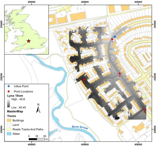
Alcester in Warwickshire experienced extensive flooding the Rivers Alne and Arrow during the floods of July 2007 in the United Kingdom, with the closest gauges on the River Arrow recording flows with a return period of 1 in 200 yr. Moreover, the local 5

drainage system was overwhelmed by excess rainfall (60–80 mm rainfall over a 12 h period). The combination of these two events led to flooding of 150 properties with both fluvial and surface water, although the Environment Agency of England and Wales (EA) estimate that a further 200 properties were successfully protected by the current flood defences. Furthermore, the EA estimates that∼260 properties in Alcester lie within the 10

1-in-100 yr floodplain (≥1 % chance of fluvial flooding each year) and substantial areas of the town are at risk from surface water. In response to this flooding, the height of the flood wall in Alcester has been increased to ensure that it is above the July 2007 river levels and two new pumping stations have been installed to expel water from the town when the drainage system capacity is exceeded (EA, 2013). The section of Alcester 15

chosen for this study lies in an area susceptible to flooding both from the River Arrow and surface water overwhelming the drainage system. The motivation for the terrestrial LiDAR collection, therefore, was to understand the detailed hydraulics of water flow in this region. The test site has an area of 0.1 km2and consists of 4 streets with a number of cul-de-sacs feeding offthem (Fig. 1).

20

Although the area selected is prone to flooding from fluvial and surface water sources, there are no reliable estimates of flood volumes for an observed flood event in the area. As the aim of this study is to determine scale and roughness effects for ter-restrial LiDAR data in urban modelling, rather than to develop a detailed understanding of flood risk at Alcester, the model boundary conditions need to be su_fficiently realistic 25

(8)

HESSD

10, 5903–5942, 2013

H. Ozdemir et al.

Title Page

Tables Figures

◭ ◮

Back Close

Full Screen / Esc

Discussion

P

a

per

|

Dis

cussion

P

a

per

|

Discussion

P

a

per

|

Discussio

n

P

a

per

|

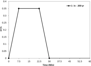
volume 2 of the UK Flood Estimation Handbook, with local parameters derived from the accompanying Flood Estimation Handbook CD-ROM (FEH, Institute of Hydrology, 1999). For this study, we assume that the 200 yr 30 min rainfall (47 mm) is collected over a drainage area of 100×100 m upstream of the inflow point (see Fig. 1) to repre-sent the flow coming from a blocked culvert opening draining a small catchment. The 5

accumulated volumes have been transformed into the simple 30 min inflow hydrograph shown in Fig. 2, where we assume inflow to increase linearly from 0 m3s−1 to peak rate over the initial 7.5 min of the event, remaining at the peak rate for the subsequent 15 min before falling linearly back to 0 m3s−1 over the final 7.5 min. The final assump-tion in this study is that the drainage system is operating at capacity such that water on 10

the surface does not interact with the drains at the road side. Whilst observed data of the flooding would be of value, its absence does not limit the present study whose aim is to understand scaling effects for terrestrial laser data using a sensitivity analysis.

2.2 Terrestrial LiDAR data collection and processing

The high resolution elevation data of Alcester used in this study were collected by the 15

Environment Agency Geomatics Group using the LYNX Mobile Mapper™ system

dis-tributed by Optech Incorporated. The LYNX Mobile Mapper™ consists of two 100 kHz

LiDAR instruments, each with 360◦ field of view, mounted on a rigid platform on the back of a Land Rover. Two GPS receivers are mounted on the roof of the car, one at the front and one on the rigid platform at the back. In addition, an inertial measurement 20

unit (IMU) is centred on the rigid platform and a sensor is mounted on the wheel to record rotations and steering direction in order to provide dead reckoning estimates of position if the GPS signal is weak. The GPS system uses the principle of real time kinematic (RTK) navigation whereby the roving LYNX unit calculates a relative position

based on a known base station with accuracies of ±5 cm. The system is capable of

25

(9)

HESSD

10, 5903–5942, 2013

H. Ozdemir et al.

Title Page

Tables Figures

◭ ◮

Back Close

Full Screen / Esc

Discussion

P

a

per

|

Dis

cussion

P

a

per

|

Discussion

P

a

per

|

Discussio

n

P

a

per

|

The terrestrial LiDAR point cloud is processed into a DEM using proprietary pro-cessing algorithms developed by EA. The main purpose of LiDAR segmentation is to separate ground hits from surface objects such as vegetation and buildings returns. However in terrestrial LiDAR surveys there is an additional need to separate long range points caused by reflection offcar surfaces and the interior of buildings from the ground 5

pulse hits. This is achieved using classification algorithms in an iterative procedure in order to progressively remove surface objects from the underlying surface topography (see for detail Sampson et al., 2012). The resulting surface was aggregated to a raster DEM at 10 cm resolution (3 616 663 cells) then resampled to 50 cm (144 659 cells) and 1 m (36 242 cells) using a simple nearest neighbour resample method (Fewtrell et al., 10

2008) to investigate the scale dependency of flooding at this site.

2.3 Model description

LISFLOOD-FP is a software package designed to model the propagation of water over complex topography typically represented by raster data. The package is a mature system that has undergone extensive development and testing since conception (e.g. 15

Bates and De Roo 2000; Hunter et al., 2005; Bates et al., 2010). The current version (Version 5.7.6) consists of a collection of numerical schemes implemented to solve a variety of mathematical approximations of the 2-D shallow water equations of different complexity (ranging from an extremely simple diffusive wave model to a shock capturing Godunov-type scheme based on the Roe Riemann solver which solves the full shallow 20

water equations (Roe, 1981; Toro, 1999, 2001; LeVeque, 2002; Willanueva and Wright, 2005). Among these different formulations, that proposed by Bates et al. (2010) has attracted increasing attention for modelling flood propagation over large urban areas. It solves a simplified inertial version of the Saint-Venant equations (e.g. Ponce, 1990; Xia, 1994; Aronica et al., 1998; Bates et al., 2010; de Almeida et al., 2012) which 25

(10)

HESSD

10, 5903–5942, 2013

H. Ozdemir et al.

Title Page

Tables Figures

◭ ◮

Back Close

Full Screen / Esc

Discussion

P

a

per

|

Dis

cussion

P

a

per

|

Discussion

P

a

per

|

Discussio

n

P

a

per

|

∂h ∂t +

∂q

∂x =0 (1)

∂q ∂t +gh

∂(h+z) ∂x +

gn2q2

h7/3 =0 (2)

whereq[L2T−1] is the discharge per unit width,h[L] is the water depth,z[L] is the bed elevation,g [L T−2] is the acceleration due to gravity,n[T L−1/3] is the Manning friction 5

coefficient, x [L] is the longitudinal coordinate and t [T] is the time. These equations were originally solved using a simple finite difference scheme applied to a staggered structured grid of square cells, which leads to a system of two explicit equations (Bates et al., 2010). Previous applications of this formulation have reported problems of nu-merical instability in domains with relatively low friction (typicallyn <0.03), which im-10

poses particular limitations to simulations of urban areas, where smooth surfaces are typically abundant.

de Almeida et al. (2012) proposed a modification of the Bates et al. (2010) numerical scheme that significantly stabilizes the solution in these low friction scenarios. The resulting model provides a robust solution to flood propagation problems over complex 15

topographies at very low computational cost. In this scheme, water flux at the interfaces of two adjacent cells is calculated using the following discretization of the simplified momentum conservation equation (Eq. 2):

qn+1

i−1/2=

θqn_i₋₁_/₂+(1−₂θ)q_in₋₃_/₂+q_in +1/2

−gh_f∆t

∆x y n i −y

n i−1

1+g∆tn 2_qn

i−1/2

h7_f/3

(3)

whereh_f is defined as the difference between max (y_i,y_i−1) and max (zi, zi−1), and

20

(11)

HESSD

10, 5903–5942, 2013

H. Ozdemir et al.

Title Page

Tables Figures

◭ ◮

Back Close

Full Screen / Esc

Discussion

P

a

per

|

Dis

cussion

P

a

per

|

Discussion

P

a

per

|

Discussio

n

P

a

per

|

2012). The subindexi denotes the centre of a computational cell andi−1/2andi−3/2the

three cell interfaces used by the numerical scheme. The superindexnandn+1 denote the indices of two time steps of the computation. Water depths inside cells are sub-sequently updated by substituting these flows into the discretized mass conservation equation:

5

y_in+1=y_in+ ∆t ∆x(q

n+1

i−1

2

−qn+1

i+1 2

). (4)

The stability is controlled by the Courant–Freidrichs–Levy conditions (e.g. Cunge, 1980) for shallow water flows:

Cr=

λ∆t

∆x (5)

where the dimensionless Courant Number (Cr) needs to be less than 1 for stability and

10

λ=pghis the wave celerity for the simplified inertial formulation. Equation (5) provides a necessary but not sufficient condition for model stability, and the model estimates the time step as:

∆t=∝ ∆x

p

ghmax

(6)

wherehmaxis the maximum depth within the computational domain andαis coefficient

15

that provides a further limitation on the maximum time step. The current version of the model uses a default value forα of 0.7, although this can be tuned by the user.

2.4 Model applications

In order to evaluate scale and roughness effects on urban surface flood modelling, different resolution DEMs produced from terrestrial LiDAR data and Manning’s ndata 20

(12)

HESSD

10, 5903–5942, 2013

H. Ozdemir et al.

Title Page

Tables Figures

◭ ◮

Back Close

Full Screen / Esc

Discussion

P

a

per

|

Dis

cussion

P

a

per

|

Discussion

P

a

per

|

Discussio

n

P

a

per

|

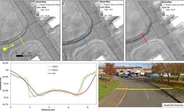
DEM data, 50 cm and 1 m resolution DEMs were derived based on the 10 cm resolution terrestrial LiDAR DEM which was used as the benchmark terrain. Figure 3 shows that little of the information (e.g. kerb and road surface camber) contained within the 10 cm terrestrial LiDAR DEM is lost when degrading to 1 m. The steepness of the kerbs is re-duced gradually and road surface camber is smoothed progressively as the resolutions 5

drops to 1 m. Representing these types of small scale features (i.e. walls, kerbs, steps, road camber) in the DEM can have significance impact especially on surface flooding in urban areas (Djokic and Maidment, 1991; Hunter et al., 2008; Fewtrell et al., 2011; Sampson et al., 2012). By contrast, Sampson et al. (2012) show that micro scale terrain features such as kerbs are not typically captured in airborne LiDAR data.

10

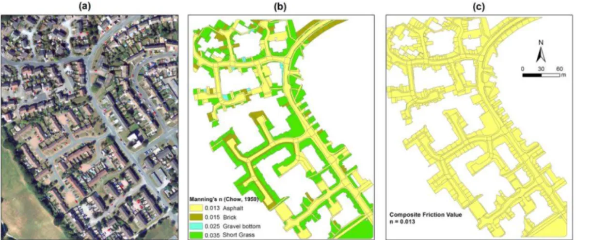
In previous studies on this test case (Fewtrell et al., 2011; Sampson et al., 2012), a single fixed composite friction coefficient was used (n=0.035) for the whole area due to large oscillations in the solution which arose at more realistic friction values when using the Bates et al. (2010) numerical solution for Eq. (2). This value (n=0.035) is likely to be too high to properly represent urban skin friction conditions. In this study, 15

we applied to the models two types of friction coefficient, namely distributed Manning’s nand a single composite friction coefficient for the entire domain (Fig. 4). Distributed

Manning’sndata were derived using UK Ordnance Survey (OS) MasterMap® vector

data. The derived data were then checked by reference to Google© satellite images and Google© street view, and any misclassified areas (such as grass classified as 20

pavement in the MasterMap®data) were manually corrected. Manning’snvalues taken from the standard Chow table (1959) were assigned to every type of land use and then converted to 10 cm, 50 cm and 1 m raster data using the cell centred method. As shown in Fig. 4, Manning’snvalues of 0.013, 0.015, 0.025 and 0.035 were assigned to asphalt road, brick, gravel and short grass surfaces respectively. During the data-processing 25

(13)

HESSD

10, 5903–5942, 2013

H. Ozdemir et al.

Title Page

Tables Figures

◭ ◮

Back Close

Full Screen / Esc

Discussion

P

a

per

|

Dis

cussion

P

a

per

|

Discussion

P

a

per

|

Discussio

n

P

a

per

|

and impervious road surfaces that typically underlie flow paths taken by surface flood water in urban areas.

In order to evaluate the different resolution terrestrial L˙IDAR DEM and roughness conditions, we used the new inertial formulation of LISFLOOD-FP (de Almeida et al., 2012, Eq. 3) to simulate the urban inundation test case in Alcester, UK. The improve-5

ment introduced by this new scheme is particularly relevant in situations involving low friction surfaces, where the previous scheme (Bates et al., 2010) exhibited problems of numerical stability which can introduce additional problems of mass balance to the model. In particular, in shallow parts of the computational domain these unphysical oscillations can lead to negative values of the water depth. The current implementa-10

tion of the model handles this situation by resetting the negative values to zero so that the model can proceed to the next time step. This artificially adds water into the domain, causing mass balance errors to grow. The comparison of the mass balance error (di_fference between the net inflow through the boundaries and the change in the water volume within the domain) in different simulations can actually be used as a first 15

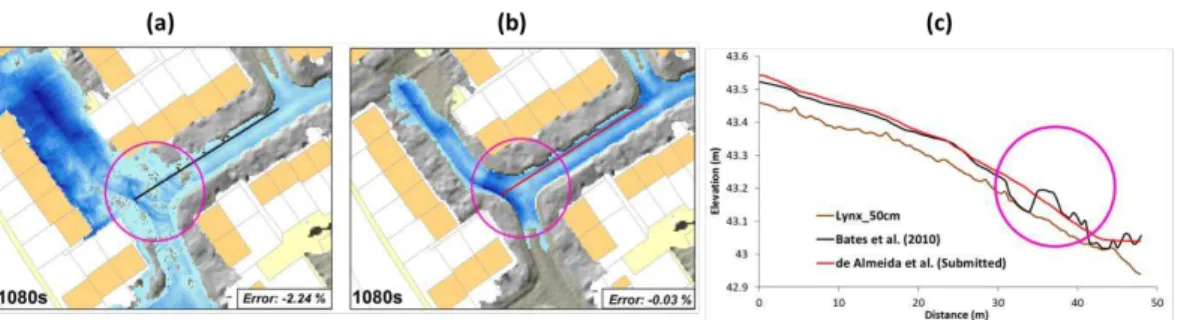
indicator of numerical stability. The previous inertial formulation developed by Bates et al. (2010) was initially compared to the that by de Almeida et al. (2012) on the 50 cm LYNX DEM and one single composite low friction (n=0.013) conditions. The results obtained with the former showed non-negligible numerical oscillations (see Fig. 5) and

high per time step volume error −2.24 %. Using the same parameters, the new

im-20

proved inertial scheme (withθ=0.8) was applied to the test site. This new formulation produced an oscillation free solution with much reduced per time step volume error (−0.03 %). All the simulations for the paper were run using α of 0.7 for the time step limiter (i.e. Eq. 5), for 2 h of simulated time (30 min of inflow event followed by 90 min for the water in the domain to come to steady state).

(14)

HESSD

10, 5903–5942, 2013

H. Ozdemir et al.

Title Page

Tables Figures

◭ ◮

Back Close

Full Screen / Esc

Discussion

P

a

per

|

Dis

cussion

P

a

per

|

Discussion

P

a

per

|

Discussio

n

P

a

per

|

3 Results and discussion

3.1 Overview of simulations

Initially, two configurations (fixed and distributed Manning’sn) of the new inertial model were built for each DEM grid scale (∆x=10 cm, 50 cm and 1 m) to establish the vari-ability associated with changing resolution and different surface friction conditions. 5

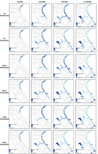
Model prediction of water depths, flood extent and flow velocity were evaluated against the relevant benchmark high-resolution (10 cm terrestrial LiDAR DEM) simulations us-ing root mean square differences (RMSD) and fit (F2) statistic (Werner et al., 2005). Figure 6 shows the propagation of the flood wave over the 10 cm, 50 cm and 1 m terres-trial LiDAR DEMs for different roughness conditions at four times (9, 24, 36, 120 min) 10

using the new inertial formulation. In all simulations, the domain is initially dry and wa-ter enwa-ters at the simulated blocked drain in the north east corner and flows down the main north-south aligned street. During the early stages of the simulations (t=9 min), water passes the first side street, which is perpendicular the main road, without flowing down it, continuing instead in a south-easterly direction. The wave front initially propa-15

gates alongside kerbs due to the representation of the road camber in the DEM, with water only spreading across the entire width of the road as water depths increase. The kerbs also serve to prevent water from spilling offthe road and towards adjacent properties until the water depth is sufficient to exceed the kerb heights. This simulated behaviour is due to the retention of the road camber within the DEM, demonstrating 20

the importance and representation capability of very high resolution DEMs in surface water flood modelling. When the flood wave reaches the second road junction, the road surface gradient causes some water to spread along the side street which runs in a south-westerly direction, whilst the remainder continues to flow along the main road which lies in a south-easterly direction (Fig. 6,t=24 min). As the simulations progress, 25

(15)

HESSD

10, 5903–5942, 2013

H. Ozdemir et al.

Title Page

Tables Figures

◭ ◮

Back Close

Full Screen / Esc

Discussion

P

a

per

|

Dis

cussion

P

a

per

|

Discussion

P

a

per

|

Discussio

n

P

a

per

|

others occur at the boundaries of the DEM that are specified as being closed in this model. The impact of road cambers being correctly represented in the terrestrial

Li-DAR DEM can also be seen clearly att=36 and 120 min, where water advancing in

a south-westerly direction down the second wetted side street flows along the road edges due to the convex profile of the road surface. Finally, water continues to drain 5

into the ponded areas until a near steady-state (t=120 min) is reached.

3.2 Sensitivity to model resolution and surface friction parameterisation

As the flood wave propagates through the street network, differences develop in the simulated water depths and inundation extent between the distributed and compos-ite friction conditions and different resolution DEMs. Maximum water depths increase 10

∼37 % when the model resolution increases from 1 m to 10 cm and surface water

speeds are reduced when using distributed friction conditions. Surface water inunda-tion is more rapid with a composite fricinunda-tion (n=0.013) and finer resolution models (Fig. 6). This latter result is opposite to the findings of Yu and Lane (2006a) for urban areas using an airborne LiDAR DEM, and occurs due to rapid propagation of water 15

along “channels” that form at the road edge as a result of the road camber and road-side kerbs. These “channels” are smoothed as resolution decreases, and consequently

water depths and velocities within them are greater on the 10 cm DEM (∼37 % and

∼32 % respectively) than the 1 m DEM. The rate of water propagation across the DEM was also tested using an idealized test case run at 10 cm, 50 cm and 1 m resolutions 20

for 60 s. The test case consists of simulating the flow of a fixed volume of water, orig-inating from a fixed point, down an idealised road represented by a long, smooth and straight surface of uniform slope, rectangular cross section and composite Manning’s nof 0.013. The distance travelled by the wave front from the fixed point of origin varied by only∼1 % between the three resolutions, indicating that the results obtained on the 25

(16)

HESSD

10, 5903–5942, 2013

H. Ozdemir et al.

Title Page

Tables Figures

◭ ◮

Back Close

Full Screen / Esc

Discussion

P

a

per

|

Dis

cussion

P

a

per

|

Discussion

P

a

per

|

Discussio

n

P

a

per

|

increased speed of wave propagation across the domain with the fixed Manning’s n

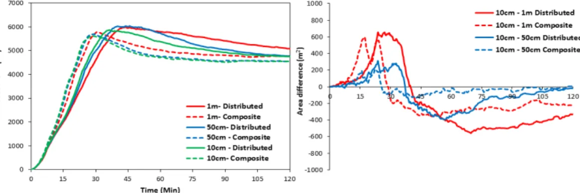
of 0.013 relative to the distributed friction map is unsurprising as an increase in sur-face friction will reduce flow velocities; however it is interesting to note that later in the simulation inundation extent is greater in models using distributed friction as water is retained for longer (Fig. 7). Therefore, during inflow to the domain, the inundated area 5

is larger in all models which use a single composite friction due to higher propagation speeds; after the inflow has ended the inundated area becomes greater in the mod-els which use distributed friction maps. In terms of maximum inundation extent, when the model resolution is increased (1 m to 10 cm), inundation extent is decreased by ∼3 % in composite friction models and ∼6 % in distributed models in this test case. 10

The area di_fference plot in Fig. 7 clearly demonstrates the e_ffects of both grid reso-lution and friction parameterisation on water propagation across the domain. During the inflow period (t <30 min), inundation area is greater in high resolution models em-ploying the composite friction map as water propagates across the DEM more quickly under these conditions. After the inflow period this pattern is reversed, as water drains 15

to depressions in the DEM (thus reducing inundation area) more quickly in the same high resolution models employing the composite friction map.

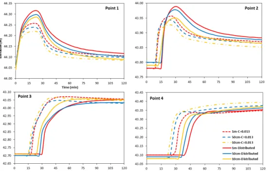
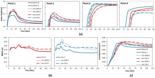
Figures 8 and 9 show the evolution of water depths and elevations, and the effects of different roughness, at four control points (see Fig. 1) through the simulation using composite and distributed friction conditions at grid resolutions of 10 cm, 50 cm and 20

1 m. Point 1 represents an area of rapid flow where water runs down a steep section of road, point 2 represents a junction where water flow splits between two streets, and points 3 and 4 are areas where ponding occurs. The water depths are higher in models using distributed roughness conditions at points 1 (∼23 %) and 2 (∼13 %), but the op-posite is observed after approximately 30 min at points 3 and 4 where the models using 25

(17)

HESSD

10, 5903–5942, 2013

H. Ozdemir et al.

Title Page

Tables Figures

◭ ◮

Back Close

Full Screen / Esc

Discussion

P

a

per

|

Dis

cussion

P

a

per

|

Discussion

P

a

per

|

Discussio

n

P

a

per

|

and composite friction models can be seen at points 2 to 4 in Figs. 8 and 9. Time delay in the distributed roughness models (relative to the composite models) reaches 12 min in this test case, despite the farthest points (3–4) being located only 300 m from the inflow point. For the distributed and composite friction configurations arrival times increase as resolution decreases, with a similar increase in time delay between the 5

friction configurations also being observed. For instance, when using the composite friction model, arrival time to point 4 is 24 min at 10 cm resolution, increasing to 30 min at 1 m resolution. For the distributed friction model, surface water reaches point 4 in 36 min at 10 cm resolution, increasing to 42 min for the 1 m model. It should also be noted from Fig. 8 that, despite representing flows resulting from a 1-in-200 yr rainfall 10

event, simulated water depths in areas of ponding along streets do not exceed the 0.5 m threshold that represents the minimum depth associated with vehicle damage (Wallingford, 2006). As such, the flows under discussion in this paper are all shallow in nature, allowing them to be influenced significantly by detailed surface topography.

Danger to people, vehicles, buildings and some infrastructure are assessed using 15

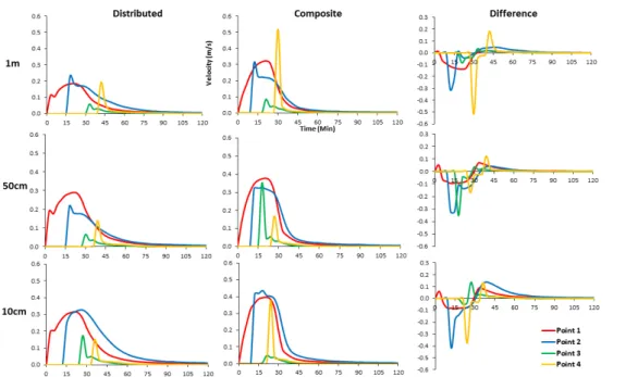
the concept of flood hazard, which can be expressed as a combination of not only water depth but also velocity (Kok et al., 2004; Kelman and Spence, 2004; Jonkman and Kelman, 2005; Wallingford, 2006; Apel et al., 2009; Xia et al., 2010, 2011). There-fore, in addition to the flood depth, velocity prediction is a valuable addition to flood studies. Fewtrell et al. (2011) and Neal et al. (2011) suggested that the simplified mod-20

els coded in LISFLOOD-FP can be used for velocity simulation for a wider range of conditions than previously thought due to the inclusion of stringent stability conditions. Figure 10 shows the evolution of the velocity at the four points throughout the simula-tion at each resolusimula-tion for both distributed and composite fricsimula-tion parameters. Velocity is calculated as the square root of the sum of the velocities in the x- and y-directions 25

(18)

HESSD

10, 5903–5942, 2013

H. Ozdemir et al.

Title Page

Tables Figures

◭ ◮

Back Close

Full Screen / Esc

Discussion

P

a

per

|

Dis

cussion

P

a

per

|

Discussion

P

a

per

|

Discussio

n

P

a

per

|

in each resolution under distributed friction conditions. These differences can be clearly summarized by comparing velocities from the 1 m distributed model to the 10 cm com-posite model in Fig. 10. In the 1 m distributed model, velocities are low and the timings of peak velocities are clearly distinct and dependent on the distance of the control point from inflow point. In the 10 cm composite model, velocities are high and thus separation 5

of peak velocities is greatly reduced, almost to the point of overlap.

3.3 Global model performance measures

In order to analyse the global effect of model resolution on simulation results, the root

mean squared di_fference (RMSD) between coarse models (50 cm and 1 m) and the

benchmark high resolution (10 cm) models for distributed and composite roughness 10

conditions are computed for depth and velocity (Fig. 11); in addition the fit statistic (F2, Werner et al., 2005) is calculated for inundated area. 50 cm and 1 m composite mod-els are compared to the 10 cm composite benchmark and 50 cm and 1 m distributed models are compared to the 10 cm distributed benchmark. There is a detectable reduc-tion in model performance at coarse resolureduc-tion which was previously noted by Horritt 15

and Bates (2001), Yu and Lane (2006a) and Fewtrell et al. (2008, 2011). In this test case, RMSD is typically higher and F2 is lower in the 1 m models than in the 50 cm models, both in terms of water depth and velocity over the simulation period. In terms of distributed and composite roughness conditions, RMSDs of water depth are lower (by ∼12 %) in the models using composite friction parameters at a given resolution. 20

The di_fference inF2between distributed and composite friction parameters is typically greater at 1 m than at 50 cm, especially during the early dynamic stages of the simula-tion while inflow is occurring. In the case of the RMSD of velocity, a smooth distribusimula-tion is not seen as with the RMSD of water depth. The RMSDs of velocity are typically lower (∼32 % at 1 m and∼8 % at 50 cm) in the models using distributed roughness parame-25

(19)

HESSD

10, 5903–5942, 2013

H. Ozdemir et al.

Title Page

Tables Figures

◭ ◮

Back Close

Full Screen / Esc

Discussion

P

a

per

|

Dis

cussion

P

a

per

|

Discussion

P

a

per

|

Discussio

n

P

a

per

|

The above analysis has shown that modelled water depths, inundation areas and velocities all exhibit sensitivity to friction parameterisation and changes in DEM reso-lution, even when the resolution of the coarsest DEM employed here (1 m) exceeds that typically used in urban inundation studies (Mason et al., 2007; Brown et al., 2007; Fewtrell et al., 2008; Hunter et al., 2008; Gallegos et al., 2009; Neal et al; 2009). The 5

results have shown water to propagate most quickly across the highest resolution DEM as small scale topographical features such as road camber and street kerbs encour-age the formation of small connecting “channels” that rapidly convey water across the domain. As reducing the resolution from 10 cm to 1 m smoothes these features and slows down wave propagation, an attempt to recover the 10 cm result on the 1 m grid 10

will require reduced surface friction to compensate for the loss of connectivity. This contrasts with previous studies undertaken at coarser grid scales using airborne Li-DAR data, where micro scale topographical features cannot be represented and where decreasing grid resolution led to faster wave propagation. In these previous studies the terrain smoothing effect of decreasing DEM resolution (Yu and Lane, 2006a) could po-15

tentially be compensated for by increasing surface friction. To test whether decreasing surface friction could potentially achieve the same effect here, the 1 m models were re-run with surface friction values of 50 and 1 % of the original distributed and com-posite values, with the results evaluated in terms of differences in water depth, arrival time, RMSD and inundated area from the benchmark 10 cm models (Fig. 12). The re-20

sults show that even when employing the most extreme 1 % surface friction scheme (spatially uniformn=0.00013), the coarse 1 m model was unable to compensate for the reduced connectivity and recover the water depth, arrival time or inundated area of the fine 10 cm benchmark model. Furthermore, the RMSD of the 50 and 1 % friction models is increased over the standard model during later stages of the simulation, sug-25

(20)

HESSD

10, 5903–5942, 2013

H. Ozdemir et al.

Title Page

Tables Figures

◭ ◮

Back Close

Full Screen / Esc

Discussion

P

a

per

|

Dis

cussion

P

a

per

|

Discussion

P

a

per

|

Discussio

n

P

a

per

|

camber, wall etc.) has a significant impact on flow propagation that cannot be recov-ered at coarser grid scales through surface friction parameterisation alone. Instead, we need to develop optimal ways to include hydraulically relevant information about micro scale topographic features in coarser DEMs as for the foreseeable future decimetric resolution hydraulic models of whole city regions may be computationally prohibitive. 5

3.4 Model stability and runtime analysis

With regard to model stability, Bates et al. (2010) highlighted that care should be taken when using the inertial formulation for large areas where low surface friction dominate due to increased instabilities, which represented an important obstacle for the applica-tion of this equaapplica-tion set for modeling flow in urban areas. However, the new formulaapplica-tion 10

proposed by de Almeida et al. (2012) considerably reduces spurious oscillations and mass errors on the finer resolution DEMs (i.e. 50 and 10 cm) and under low friction conditions. In our simulations this was achieved by adding a relatively small amount of numerical diffusion to the method (e.g.θbetween 0.9 and 0.7). The computational cost of running the simulation under distributed or composite friction conditions was similar. 15

As expected, changing the resolution had a significant impact on computational time. Runtimes for the 1-in-200 yr event at 10 cm, 50 cm and 1 m scales for 0.1 km2 area were typically∼90 h,∼21 min and∼5 min respectively using a Quad core Intel Core i7 CPU Q740 1.73 GHz processor. Hence, as previously noted by Sampson et al. (2012), the current version of LISFLOOD-FP would not be appropriate for large-scale urban 20

flood modelling using very fine resolution DEMs of 10 cm or below. There is increas-ing interest in undertakincreas-ing hydraulic modellincreas-ing over very large domains (Pappenberger et al., 2009; Merz et al., 2010), and continued development of efficient hydraulic code, as well as methods for efficient use of topographic data, will be required to achieve this aim.

(21)

HESSD

10, 5903–5942, 2013

H. Ozdemir et al.

Title Page

Tables Figures

◭ ◮

Back Close

Full Screen / Esc

Discussion

P

a

per

|

Dis

cussion

P

a

per

|

Discussion

P

a

per

|

Discussio

n

P

a

per

|

4 Conclusions

This paper presents applications and benchmark testing results of a new inertial for-mulation of LISFLOOD–FP using distributed and composite friction conditions on high resolution terrestrial LIDAR DEMs (10 cm, 50 cm and 1 m) in Alcester, UK. This repre-sents the first attempts at conducting hydraulic modelling using sub-meter scale (10 cm, 5

50 cm and 1 m) elevation data derived from terrestrial LiDAR data in conjunction with realistic friction conditions (n <0.03). The water depth, inundation extent, arrival time and velocity predicted by the simulations were shown to vary in response to DEM reso-lution and different friction conditions. Maximum water depths and velocity are shown to increase by up to∼37 and∼32 % respectively with increasing DEM resolution, whilst 10

inundation extent is shown to decrease by approximately 6 %. A further idealised sim-ulation is used to confirm that the results are grid independent and due to the ability of terrestrial LIDAR to resolve small scale features missed by airborne LIDAR due to its use of a sideways looking laser system with∼1–3 cm point spacing. During a sur-face flooding event, the formation of flow “channels” constrained by small scale features 15

such as road cambers and kerbs is observed in simulations run on the fine scale terres-trial LIDAR DEMs. These channels improve hydraulic connectivity across the domain, allowing water to drain rapidly to depressions where ponding occurs.

In order to investigate the e_ffects of surface roughness parameterisation, two sur-face friction configurations (a uniform composite value and a variable distributed fric-20

tion map) were applied to all resolution DEMs of the Alcester test site and the im-pact on flood depth, flood extent, flood arrival times and velocity were evaluated. Land use classes for friction conditions were derived from UK Ordnance Survey (OS) MasterMap® data with some editing using Google© satellite images and Street View. The results showed flood extent to be less sensitive to surface friction configuration 25

(22)

HESSD

10, 5903–5942, 2013

H. Ozdemir et al.

Title Page

Tables Figures

◭ ◮

Back Close

Full Screen / Esc

Discussion

P

a

per

|

Dis

cussion

P

a

per

|

Discussion

P

a

per

|

Discussio

n

P

a

per

|

distributions (Mason et al., 2003; Begnudelli and Sanders, 2007). However, recovering the result of the finest grid resolution simulation on the coarser DEM by changing the surface friction is shown not to be possible at this site. This is because flow propa-gation at the finest grid resolution is not only related to the surface friction values but also to the representation of hydraulically relevant small scale topographical features 5

in the DEM. Reducing the resolution of the DEM reduces the capacity to represent these features and leads to a loss in modelling hydraulic connectivity across the do-main, something that cannot here be compensated for by changing the surface friction parameterisation. We conclude that micro scale terrain features are therefore relatively more important to flood wave development because they create or block flow pathways 10

rather than because they are generate frictional losses.

The new numerical solution for the Bates et al. (2010) equations proposed by de Almeida et al. (2012) demonstrated increased model stability on high resolution DEMs under low friction conditions (n=0.013) compared to the previous scheme, although it reduced computational efficiency at 10 cm resolution. The new formulation was also 15

seen to solve the instabilities caused by low friction conditions on areas with shallow slopes. However, instability can also originate on high gradient slopes where super-critical flow occurs and this may be outside the ability of simpler schemes to simulate as these often strictly apply to subcritical flows only (Neal et al., 2011). Future work should concentrate on increasing the computational performance of simplified shallow 20

water models on finer resolution DEMs (10 cm or below) and improving their ability to simulate supercritical flows for high gradient terrain features which may be common in urban environments.

The paper has shown that fine scale terrain data are required for the simulation of shallow surface water flows in urban environments. This finding suggests that terrestrial 25

(23)

HESSD

10, 5903–5942, 2013

H. Ozdemir et al.

Title Page

Tables Figures

◭ ◮

Back Close

Full Screen / Esc

Discussion

P

a

per

|

Dis

cussion

P

a

per

|

Discussion

P

a

per

|

Discussio

n

P

a

per

|

Drainage Systems (SUDS) are being considered, as precise simulation of surface wa-ter flow will facilitate the planning and implementation of SUDS techniques such as source control, permeable conveyance systems and temporary storm water storage solutions (DEFRA, 2004). Whilst a complete SUDS design analysis for a site could not be completed without coupling the model to a sewer model able to represent the 5

typically employed overflow pipe system, an uncoupled model would still be of value at the planning stage to identify areas most at risk from surface water flooding, as well as when considering remedial flood drainage for when the system capacity is exceeded. Unfortunately, simulation at decimetric scales remains computationally expensive even when using efficient state-of-the-art hydraulic models, so it is suggested that future 10

research should focus on further increasing the e_fficiency of such models as well as developing techniques that enable the representation of key hydraulically relevant small scale features at coarser resolutions

Acknowledgements. Hasan Ozdemir was funded by TUBITAK (The Scientific and Technolog-ical Research Council of Turkey) with program of 2219. The work forms part of Christopher

15

Sampson’s PhD research at the University of Bristol funded by a Natural Environment Re-search Council (NERC) Combined Award in Science and Engineering (NE/H017836/1) in part-nership with the Willis Research Network (WRN). The authors would like to thank Paul Smith and James Whitcombe of the Environment Agency Geomatics Group for helping the authors understand LiDAR surveying with LYNX in practice.

20

References

Apel, H., Aronica, G. T., Kreibich, H., and Thieken, A. H.: Flood risk analyses-how detailed do we need to be?, Nat. Hazards, 49, 79–98, 2009.

Aronica, G. T. and Lanza, J. G.: Drainage efficiency in urban areas: a case study, Hydrol. Process., 19, 1105–1119, 2005.

25

(24)

HESSD

10, 5903–5942, 2013

H. Ozdemir et al.

Title Page

Tables Figures

◭ ◮

Back Close

Full Screen / Esc

Discussion

P

a

per

|

Dis

cussion

P

a

per

|

Discussion

P

a

per

|

Discussio

n

P

a

per

|

Barnea, S. and Filin, S.: Keypoint based autonomous registration of terrestrial laser point-clouds, ISPRS J. Photogramm, 63, 19–35, 2008.

Bates, P. D. and De Roo, A. P. J.: A simple raster-based model for flood inundation simulation, J. Hydrol., 236, 54–77, 2000.

Bates, P. D., Stewart, M. D., Siggers, G. B., Smith, C. N., Hervouet, J. M., and Sellin, R. H. J.:

5

Internal and external validation of a two-dimensional finite element model for river flood sim-ulation, P. I. Civil. Eng.-Water, 130, 127–141, 1998.

Bates, P. D., Horritt, M. S., and Fewtrell, T. J.: A simple inertial formulation of the shallow water equations for efficient two dimensional flood inundation modelling, J. Hydrol., 387, 33–45, 2010.

10

Begnudelli, L. and Sanders, B. F.: Simulation of the St. Francis dam-break flood, J. Eng. Mech., 133, 1200–1212, 2007.

Brown, J. D., Spencer, T., and Moeller, I.: Modelling storm surge flooding of an urban area with particular reference to modelling uncertainties: a case study of Canvey Island, UK, Water Resour. Res., 43, W06402, doi:10.1029/2005WR004597, 2007.

15

Chow, V.: Open Channel Hydraulics, McGraw-Hill, New York, 1959.

Cunge, J. A., Holly, F. M., and Verwey, A.: Practical Aspects of Computational River Hydraulics, Pitman, London, UK, 420 pp., 1980.

de Almeida, G. A. M., Bates, P. D., Freer, J. E., and Souvignet, M.: Improving the stability of a simple formulation of the shallow water equations for 2D flood modelling, Water Resour.

20

Res., 48, W05528, doi:10.1029/2011WR011570, 2012.

DEFRA: Interim code of practice for Sustainable Drainage Systems, National SUDS Working Group, UK, 2004.

DEFRA: Future Water: The Government’s Water Strategy for England, CM7319, HM Govern-ment, London, 2008.

25

Djokic, D. and Maidment, D. R.: Terrain analysis for urban stormwater modelling, Hydrol. Pro-cess., 5, 115–124, 1991,

Environmental Agency (EA): available at: http://www.environment-agency.gov.uk/ homeandleisure/floods/142209.aspx (last access: 13 May 2013), 2011.

Fewtrell, T. J., Bates, P. D., Horritt, M., and Hunter, N. M.: Evaluating the effect of scale in flood

30

(25)

HESSD

10, 5903–5942, 2013

H. Ozdemir et al.

Title Page

Tables Figures

◭ ◮

Back Close

Full Screen / Esc

Discussion

P

a

per

|

Dis

cussion

P

a

per

|

Discussion

P

a

per

|

Discussio

n

P

a

per

|

Fewtrell, T. J., Duncan, A., Sampson, C. C., Neal, J. C., and Bates, P. D.: Benchmarking urban flood models of varying complexity and scale using high resolution terrestrial LiDAR data, Phys. Chem. Earth, 36, 281–291, 2011.

Gallegos, H. A., Schubert, J. E., and Sanders, B. F.: Two-dimensional, high-resolution modeling of urban dam-break flooding: a case study of Baldwin Hills California, Adv. Water Resour.,

5

32, 1323–1335, 2009.

Gee, D. M., Anderson, M. G., and Baird, L.: Large scale floodplain modelling, Earth Surf. Proc. Land., 15, 512–523, 1990.

Guinot, V. and Soares-Frazao, S.: Flux and source term discretization in two-dimensional shal-low water models with porosity on unstructured grids, Int. J. Numer. Meth. Fl., 50, 309–345,

10

2006.

Horritt, M. S.: Calibration of a two-dimensional finite element flood flow model using satellite radar imagery, Water Resour. Res., 36, 3279–3291, 2000.

Horritt, M. S. and Bates, P. D.: E_ffect of spatial resolution on a raster based model of flood flow, J. Hydrol., 253, 239–249, 2001.

15

Horritt, M. S. and Bates, P. D.: Evaluation of 1D and 2D numerical models for predicting river flood inundation, J. Hydrol., 268, 87–99, 2002.

Hsu, M. H., Chen, S. H., and Chang, T. J.: Inundation simulation for urban drainage basin with storm sewer system, J. Hydrol., 234, 21–37, 2000.

Hunter, N. M., Horritt, M. S., Bates, P. D., Wilson, M. D., and Werner, M. G. F.: An adaptive time

20

step solution for raster-based storage cell modelling of floodplain inundation, Adv. Water Resour., 28, 975–991, 2005.

Hunter, N. M., Bates, P. D., N ´eelz, S., Pender, G., Villanueva, I., Wright, N. G., Liang, D., Fal-coner, R. A., Lin, B., Waller, S., Crossley, A. J., and Mason, D. C.: Benchmarking 2D hydraulic models for urban flooding, P. I. Civil. Eng.-Wat. M., 16, 13–30, 2008.

25

Institute of Hydrology: Flood Estimation Handbook, Institute of Hydrology, Wallingford, 1999. Jonkman, S. N. and Kelman, I.: An analyses of the causes and circumstances of flood disaster

deaths, Disasters, 29, 75–97, 2005.

Kelman, I. and Spence, R.: An overview of flood actions on buildings, Eng. Geol., 73, 297–309, 2004.

30

(26)

HESSD

10, 5903–5942, 2013

H. Ozdemir et al.

Title Page

Tables Figures

◭ ◮

Back Close

Full Screen / Esc

Discussion

P

a

per

|

Dis

cussion

P

a

per

|

Discussion

P

a

per

|

Discussio

n

P

a

per

|

LeVeque, R. J.: Finite Volume Methods for Hyperbolic Problems, Cambridge Univ. Press, Cam-bridge, Mass., 257 pp., 2002.

Lichti, D., Pfeifer, N., and Maas, H.: ISPRS Journal of Photogrammetry and Remote Sensing theme issue “Terrestrial Laser Scanning”, ISPRS J. Photogramm., 63, 1–3, 2008.

Mason, D. C., Cobby, D. M., Horritt, M. S., and Bates, P. D.: Floodplain friction parametrization in

5

two-dimensional river flood models using vegetation heights derived from airborne scanning laser altimetry, Hydrol. Process., 17, 1711–1732, 2003.

Mason, D. C., Horritt, M. S., Hunter, N. M., and Bates, P. D.: Use of fused airborne scanning laser altimetry and digital map data for urban flood modelling, Hydrol. Process., 21, 1436– 1447, 2007.

10

Merz, B., Hall, J., Disse, M., and Schumann, A.: Fluvial flood risk management in a changing world, Nat. Hazards Earth Syst. Sci., 10, 509–527, doi:10.5194/nhess-10-509-2010, 2010. Mignot, E., Paquier, A., and Haider, S.: Modeling floods in a dense urban area using 2D shallow

water equations, J. Hydrol., 327, 186–199, 2006.

Neal, J. C., Bates, P. D., Fewtrell, T. J., Hunter, N. M., Wilson, M. D., and Horritt, M. S.:

Dis-15

tributed whole city water level measurement from the Carlisle 2005 urban flood event and comparison with hydraulic model simulations, J. Hydrol., 368, 42–55, 2009.

Neal, J. C., Villanueva, I., Wright, N., Willis, T., Fewtrell, T., and Bates, P. D.: How much phys-ical complexity is needed to model flood inundation?, Hydrol. Process., 26, 2262–2282, doi:10.1002/hyp.8339, 2011.

20

N ´eelz, S. and Pender, G.: Benchmarking of 2D Hydraulic Modelling Packages, SC080035/R2 Environment Agency, Bristol, 2010.

N ´eelz, S., Pender, G., Villanueva, I., Wilson, M., Wright, N. G., Bates, P., Mason, D., and Whit-low, C.: Using remotely sensed data to support flood modelling, P. I. Civil. Eng.-Wat. M., 159, 35–43, 2006.

25

Nicholas, A. P. and Mitchell, C. A.: Numerical simulation of overbank processes in topographi-cally complex floodplain environments, Hydrol. Process., 17, 727–746, 2003.

Pappenberger, F., Cloke, H. L., Balsamo, G., Ngo-Duc, T., and Oki, T.: Global runo_ffrouting with the hydrological component of the ECMWF NWP system, Int. J. Climatol., 30, 2155–2174, 2009.

30

(27)

HESSD

10, 5903–5942, 2013

H. Ozdemir et al.

Title Page

Tables Figures

◭ ◮

Back Close

Full Screen / Esc

Discussion

P

a

per

|

Dis

cussion

P

a

per

|

Discussion

P

a

per

|

Discussio

n

P

a

per

|

Ponce, V. M.: Generalized diffusion wave equation with inertial effects, Water Resour. Res., 26, 1099–1101, 1990.

Roe, P. L.: Approximate riemann solvers, parameter vectors and difference schemes, J. Com-put. Phys., 43, 357–372, 1981.

Sampson, C. C., Fewtrell, T. J., Duncan, A., Shaad, K., Horritt, M. S., and Bates, P. D.: Use of

5

terrestrial laser scanning data to drive decimetric resolution urban inundation models, Adv. Water Resour., 41, 1–17, 2012.

Schubert, J. E., Sanders, B. F., Smith, M. J., and Wright, N. G.: Unstructured mesh generation and landcover-based resistance for hydrodynamic modeling of urban flooding, Adv. Water Resour., 31, 1603–1621, 2008.

10

Toro, E. F.: Riemann Solvers and Numerical Methods for Fluid Dynamics, Springer-Verlag, 1999.

Toro, E. F.: Shock-capturing methods for free-surface shallow flows, John Wiley and Sons, LTD., 2001.

Tsubaki, R. and Fujita, I.: Unstructured grid generation using LiDAR data for urban flood

inun-15

dation modelling, Hydrol. Process., 24, 1404–1420, 2010.

Villauneva, I. and Wright, N. G.: Linking Riemann and storage cell models for flood prediction, Water Manage., 159, 27–33, 2005.

Wallingford, H. R.: Flood Risk to People Phase 2, FD2321/TR2 Guidance Document, De-fra/Environmental Agency, UK, 2006.

20

Werner, M. G. F., Hunter, N. M., and Bates, P. D.: Identifiability of distributed floodplain rough-ness values in flood extent estimation, J. Hydrol., 314, 139–157, 2005.

Wheater, H. S.: Progress in and prospects for fluvial flood modelling, Philos. T. Roy. Soc. A, 360, 1409–1431, 2002.

Wilson, M. D. and Atkinson, P. M.: The use of remotely sensed land cover to derive floodplain

25

friction coefficients for flood inundation modelling, Hydrol. Process., 21, 3576–3586, 2007. Xia, J., Teo, F. Y., Lin, B., and Falconer, R. A.: Formulation of incipient velocity for flooded

vehicles, Nat. Hazard, 58, 1–14, 2010.

Xia, J., Falconer, R. A., Lin, B., and Tan, G.: Modelling flash flood risk in urban areas, Water Manage., 164, 267–282, 2011.

30