Spatial analysis of precipitation in a high-mountain region: exploring methods with multi-scale topographic predictors and circulation types

(1)

HESSD

11, 4639–4694, 2014

Spatial analysis of precipitation in a high-mountain region

D. Masson and C. Frei

Title Page

Abstract Introduction

Conclusions References

Tables Figures

◭ ◮

Back Close

Full Screen / Esc

Printer-friendly Version Interactive Discussion

Discussion

P

a

per

|

D

iscussion

P

a

per

|

Discussion

P

a

per

|

Discuss

ion

P

a

per

|

Hydrol. Earth Syst. Sci. Discuss., 11, 4639–4694, 2014 www.hydrol-earth-syst-sci-discuss.net/11/4639/2014/ doi:10.5194/hessd-11-4639-2014

Hydrology and Earth System

Sciences

Open Access

Discussions

This discussion paper is/has been under review for the journal Hydrology and Earth System Sciences (HESS). Please refer to the corresponding final paper in HESS if available.

Spatial analysis of precipitation in a

high-mountain region: exploring methods

with multi-scale topographic predictors

and circulation types

D. Masson and C. Frei

MeteoSwiss, Federal Oﬃ_{ce of Meteorology and Climatology, Kraehbuehlstrasse 58,}

8044 Zurich, Switzerland

Received: 21 March 2014 – Accepted: 10 April 2014 – Published: 9 May 2014

Correspondence to: D. Masson (massond@phys.ethz.ch)

(2)

HESSD

11, 4639–4694, 2014

Title Page

Tables Figures

◭ ◮

Back Close

Full Screen / Esc

Discussion

P

a

per

|

D

iscussion

P

a

per

|

Discussion

P

a

per

|

Discuss

ion

P

a

per

|

Abstract

Statistical models of the relationship between precipitation and topography are key elements for the spatial interpolation of rain-gauge measurements in high-mountain regions. This study investigates several extensions of the classical precipitation-height model in a direct comparison and within two popular interpolation frameworks, namely

5

linear regression and kriging with external drift. The models studied include predictors of topographic height and slope, eventually at several spatial scales, a stratification by types of a circulation classification, and a predictor for wind-aligned topographic gra-dients. The benefit of the modeling components is investigated for the interpolation of seasonal mean and daily precipitation using leave-one-out crossvalidation. The study

10

domain is a north-south cross-section of the European Alps (154 km×187 km), which disposes of dense rain-gauge measurements (approx. 440 stations, 1971–2008).

The significance of the topographic predictors was found to strongly depend on the interpolation framework. In linear regression predictors of slope and at multiple scales reduce interpolation errors substantially. But with as many as nine predictors the

result-15

ing interpolation still poorly replicates the across-ridge variation. Kriging with external drift (KED) leads to much smaller interpolation errors than linear regression. But this is achieved with a single predictor of local height already, and the extended predictor sets bring only marginal further improvement. Again, the stratification by circulation types and the wind-aligned gradient predictor do not improve over the single predictor

20

KED model. Similarly for daily precipitation, information from circulation types is not improving interpolation accuracy. The results confirm that topographic predictors are essential for reducing interpolation errors, but exploiting the spatial autocorrelation in the data may be as eﬀ_{ective as developing elaborate predictor sets. Our results also}

question a popular practice of using linear regression for predictor selection and they

25

(3)

HESSD

11, 4639–4694, 2014

Title Page

Tables Figures

◭ ◮

Back Close

Full Screen / Esc

Discussion

P

a

per

|

D

iscussion

P

a

per

|

Discussion

P

a

per

|

Discuss

ion

P

a

per

|

1 Introduction

High-mountain ranges contribute to the supply and storage of freshwater and river flow in many regions of the world (e.g. Viviroli et al., 2007). The role of mountains in ex-tracting moisture from the atmosphere manifests in numerous regional anomalies and gradients in the distribution of the global precipitation climate (e.g. Basist et al., 1994;

5

Schneider et al., 2013). Accurate knowledge of the distribution and variation of rain and snowfall is crucial for numerous planning tasks concerned, for example, with water resources, water power, agriculture, glaciology and natural hazards (e.g. Greminger, 2003; Holzkamper et al., 2012; Machguth et al., 2009; Yates et al., 2009). A conve-nient source of information are spatial analyses of observed precipitation, obtained by

10

interpolation onto a regular grid, comprehensively over large areas. Such grid datasets have become of interest also for monitoring climate variations and for evaluating model-based re-analyses and climate models (e.g. Alexander et al., 2006; Bukovsky and Karoly, 2007; Frei et al., 2003; Schmidli et al., 2002).

The construction of accurate precipitation grid datasets for high-mountain regions is

15

confronted with the challenge of complex spatial variations. Even with idealized topo-graphic settings and flow configurations (e.g. isolated hill or ridge, constant flow), situa-tions can be distinguished where precipitation maxima occur over the windward slope, over the crest or the downwind slope of a topographic obstacle (e.g. Sinclair et al., 1997; Smith, 1979). Distributions depend on the height and scale of the obstacle, and

20

the strength, static stability and moisture profile of the impinging flow. More complex topographic shapes, transient weather systems, convection and the drift of hydrome-teors quickly complicate the picture (e.g. Cosma et al., 2002; Fuhrer and Schär, 2005; Houze et al., 2001; Roe, 2005; Sinclair et al., 1997; Steiner et al., 2003). Therefore, the distribution of long-term mean precipitation is, in many regions, a superposition of

25

several distinct responses to topography, which act at diﬀ_{erent space scales, involve}

several characteristics of the topography (not just height) and pertain to diﬀ_{erent flow}

(4)

HESSD

11, 4639–4694, 2014

Title Page

Tables Figures

◭ ◮

Back Close

Full Screen / Esc

Discussion

P

a

per

|

D

iscussion

P

a

per

|

Discussion

P

a

per

|

Discuss

ion

P

a

per

|

A further complication for spatial analysis in mountain regions is posed by the limited spatial density of rain gauges, the standard device for climatological inference on pre-cipitation. Even in comparatively densely instrumented areas, such as the European Alps, the networks do not resolve contrasts between individual valleys and hills ex-plicitly, and they miss out episodic fine-scale patterns familiar from radar observations

5

and numerical models (e.g. Bergeron, 1961; Frei and Schär, 1998; Germann and Joss, 2001; Zangl et al., 2008). Moreover, the distribution of rain gauges in complex terrain is often biased, with a majority of measurements taken at valley floors, while steep slopes and high elevations are underrepresented (e.g. Frei and Schär, 1998; Sevruk, 1997). The sampling bias entails a risk of systematic errors in spatial interpolation, which can

10

impinge upon estimates at larger scale, such as for averages over river catchments (e.g. Daly et al., 1994; Sinclair et al., 1997).

In this context, models of the relationship between precipitation and topography constitute an essential element of spatial interpolation methods. Their purpose is to enhance the methods’ capabilities in describing variations not explicitly resolved by

15

the observations, and to reduce the risk of systematic errors related to the non-representativity of the measurement network. Approaches for considering precipitation-topography relationships in interpolation methods can roughly be grouped into

empir-ical statistempir-ical models using more or less extensive sets of physiographic predictors

(e.g. Benichou and Le Breton, 1986; Daly et al., 1994; Prudhomme and Reed, 1998)

20

and simplifiedphysico-dynamical downscaling modelsin combination with information on larger-scale circulation (e.g. Crochet et al., 2007; Sinclair, 1994).

In this study we explore and compare several ideas for the modeling of precipitation-topography relationships in the framework of empirical statistical models. Our specific focus is on models that (a) take account of the multi-scale nature of the relationship,

25

(b) consider responses both to slope and elevation of the topography, (c) involve a de-pendency on the direction of the large-scale flow, and (d) examine the potential of a stratification by circulation types. The value of the diﬀ_{erent modeling components is}

(5)

HESSD

11, 4639–4694, 2014

Title Page

Tables Figures

◭ ◮

Back Close

Full Screen / Esc

Discussion

P

a

per

|

D

iscussion

P

a

per

|

Discussion

P

a

per

|

Discuss

ion

P

a

per

|

models incorporated and is applied for the estimation of fields of seasonal mean and daily precipitation in a sub-region of the European Alps.

Systematic topography eﬀ_{ects on precipitation are usually di}ﬃ_{cult to discern in}

obser-vations at short time scales (e.g. for daily totals). Precipitation-topography relationships are therefore mostly estimated from long-term averages, which are then used, via a

cli-5

matological background field, for the interpolation of shorter duration totals (Haylock et al., 2008; Rauthe et al., 2013; Widmann and Bretherton, 2000).

A common model of topography eﬀ_{ects is that of a linear relationship between}

clima-tological (seasonal or monthly) mean precipitation and in-situ topographic elevation. Precipitation-height gradients have been considered in various interpolation

method-10

ologies such as in linear regression by using height as a predictor (e.g. Gottardi et al., 2012; Rauthe et al., 2013; Sokol and Bliž_{nák, 2009) in several variants of kriging by}

using a digital elevation model as secondary variable (Goovaerts, 2000; Hevesi et al., 1992; Phillips et al., 1992), in thin-plate splines interpolation by using height as a third regionalization variable (Haylock et al., 2008; Hutchinson, 1998) or in triangular

inter-15

polation by adopting height corrections (Tveito et al., 2005). The assumption of these procedures is that local height is a key explanatory variable of the distribution of pre-cipitation and that the relationship, commonly estimated over larger domains, is rep-resentative at the scale relevant for the interpolation, i.e. at and below the spacing of stations.

20

Three types of extensions of the aforementioned methodologies have been pro-posed: the first introduced a range of physiographic predictors (not just height) and/or predictors representing smoothed versions of the actual topography (e.g. Basist et al., 1994; Benichou and Le Breton, 1986; Gyalistras, 2003; Perry and Hollis, 2005; Prudhomme and Reed, 1998; Sharples et al., 2005). Additional predictors (e.g. slope,

25

(6)

HESSD

11, 4639–4694, 2014

Title Page

Tables Figures

◭ ◮

Back Close

Full Screen / Esc

Discussion

P

a

per

|

D

iscussion

P

a

per

|

Discussion

P

a

per

|

Discuss

ion

P

a

per

|

and Reed, 1998; Sharples et al., 2005). Conversely, the second extension remains with univariate height dependencies, but considers the relationship to be spatially vari-able (Brunetti et al., 2012; Daly et al., 1994; Gottardi et al., 2012). The aim is to focus on dependencies at scales that are not explicitly resolved by the station network and, hence, are particularly relevant for interpolation. There are diﬀ_{erent emphases in the}

5

two extensions between robustness and local representativity of the precipitation to-pography model used for interpolation.

The third type of extending traditional precipitation height models is to incorporate in-formation on atmospheric flow conditions into the interpolation: Kyriakidis et al. (2001) have constructed new rainfall predictors by combination of lower-atmosphere flow and

10

moisture with local terrain height and slope. When used in kriging these dynamical pre-dictors yielded more accurate interpolations of the seasonal mean precipitation com-pared to using elevation only. Hewitson and Crane (2005) have modified the weighting scheme of a daily interpolation method to depend on synoptic state (discrete types of daily low-level circulation) in order to account for the varying short-range

representa-15

tivity of station measurements. Gottardi et al. (2012) use the circulation regime of the day under consideration to estimate orographic eﬀ_{ects specifically for di}ﬀ_{erent weather}

conditions. All these ideas are building on empirical evidence that the mesoscale pre-cipitation distribution in complex terrain varies considerably between days with diﬀ_erent

large-scale flow conditions (Cortesi et al., 2013; Schiemann and Frei, 2010).

20

In this study we build on, extend and test ideas of all three extensions in a subre-gion of the European Alps. We compare several sets of physiographic predictors with regard to their relevance for high-resolution precipitation interpolation. Apart from in-cluding height and directional gradients, our set encompasses predictors at several spatial scales simultaneously in order to explicitly distinguish between patterns

re-25

(7)

HESSD

11, 4639–4694, 2014

Title Page

Tables Figures

◭ ◮

Back Close

Full Screen / Esc

Discussion

P

a

per

|

D

iscussion

P

a

per

|

Discussion

P

a

per

|

Discuss

ion

P

a

per

|

analyses for composites of a circulation type classification and by including predictors of the pertinent circulation terrain eﬀ_{ect. Most of our analyses focus on interpolations for}

seasonal mean precipitation, but we also assess the relevance of circulation-type de-pendent background fields for the interpolation of daily precipitation. Essential for all our comparisons is that interpolation errors will be examined as a function of topographic

5

height and for both systematic and random error components. The main purpose of our study is to gain insight on the role of diﬀ_{erent approaches to precipitation-topography}

modelling, but some of our analyses also explore possibilities to improve an interpola-tion method previously developed for the generainterpola-tion of a precipitainterpola-tion grid dataset for the entire Alpine region (Isotta et al., 2013).

10

The region of the European Alps is an interesting example for studying interpolation procedures and pertinent models of the precipitation topography relationship. There is an exceptional density of long-term rain-gauge observations (see Fig. 1), which allows modeling approaches of larger complexity than in sparsely gauged mountain regions. Moreover, there is a broad range of topographic scales (from hundreds of kilometers

15

for the main ridge down to few kilometers for individual massifs) and variations in ridge height (2000–3000 m for the main ridge down to few hundred meters for adjacent hill ranges). Accordingly, the distribution of mean precipitation reveals several nested pat-terns of the precipitation response that is indicative of its multi-scale nature (see Fig. 1). This study is part of the European project EURO4M (European Reanalysis and

Ob-20

servations for Monitoring). The outline of the study is organized as follows: in Sect. 2 we introduce the study domain and the data. The methods of spatial analysis and the procedure of evaluation are described in Sect. 3. The results of the evaluation are then presented and discussed in Sect. 4 and the conclusions of this study are drawn in Sect. 5.

(8)

HESSD

11, 4639–4694, 2014

Title Page

Tables Figures

◭ ◮

Back Close

Full Screen / Esc

Discussion

P

a

per

|

D

iscussion

P

a

per

|

Discussion

P

a

per

|

Discuss

ion

P

a

per

|

2 Study domain and data

In this study we consider a sub-domain of the Alps (11–13◦E/46.85–48.5◦N) that cov-ers an area of 154 km×187 km and extends from the flatlands of Bavaria (Southern Germany), over the Northern slopes of the Alpine ridge (at the country border between Germany and Austria) towards the inner Alpine region of Tyrol (Inn and Salzach valleys,

5

Austria and Northern Italy). The domain is indicated in Fig. 1 (red frame) and a detailed topographic map is depicted in Fig. 2a. Our choice is motivated by the comparatively simple large-scale pattern of the topography here, so that the domain can be consid-ered as a cross-section through an elongated west-east oriented ridge, extending from flatlands over foothills to high mountains with major inner mountain valleys (from North

10

to South). As opposed to a larger domain with more convoluted topography, the inter-mediate complexity eases the exploration of potential physiographic predictors but still comprises the challenges encountered with distinct and typical climates of the entire Alpine ridge. In addition, the selected domain disposes of a homogenous and, com-pared to other regions, very dense coverage with rain gauges (cf. Fig. 1).

15

The rain-gauge data for this study (Fig. 2a) was obtained from the German Weather Service (DWD, for Germany), from the Austrian Federal Ministry of Agriculture, Forestry, Environment and Water (for Austria) and from Servizio Meteorologico and Uﬃ_{cio Idrografico Bolzano Alto Adige (for Italy). The dataset is a subset of 440 stations}

out of a pan-Alpine compilation of high-resolution daily rain-gauge time series

extend-20

ing over the period 1971–2008 (Isotta et al., 2013). On average the station density is 1 station per 70 km2 corresponding to a typical inter-station distance of 8.5 km, a very dense coverage over a high-mountain region.

Like in other mountainous regions, the distribution of the stations in our study domain has a limited representativity with respect to terrain height (Fig. 2b). High-elevation

ar-25

(9)

HESSD

11, 4639–4694, 2014

Title Page

Tables Figures

◭ ◮

Back Close

Full Screen / Esc

Discussion

P

a

per

|

D

iscussion

P

a

per

|

Discussion

P

a

per

|

Discuss

ion

P

a

per

|

areas being biases due to inappropriate interpolation between valley stations. This will be given particular attention in the assessment of interpolation methods later.

The rain-gauge time series underwent diﬀ_{erent quality control procedures at the}

orig-inal data providers. In addition they were rigorously checked for raw errors, jointly af-ter compilation, using criaf-teria of temporal and spatial consistency and physical

plau-5

sibility (for details see Isotta et al., 2013). One caveat of the quality of the data is, however, posed by the systematic measurement error emanating from wind-induced under-catch, wetting and evaporation losses (Groisman and Legates, 1994; Neﬀ_{, 1977;}

Sevruk, 2005). Sevruk (1985) and Richter (1995) estimate the systematic measure-ment error in the Alps to range from about 7 % (5 %) over the flatland regions in winter

10

(summer) to 30 % (10 %) above 1500 mMSL The data used in this study is not corrected for these systematic errors. Indeed, water balance considerations in the Alps have chal-lenged existing correction procedures (Schädler and Weingartner, 2002; Weingartner et al., 2007). The systematic errors may aﬀ_{ect the strength and estimation of}

empir-ical precipitation topography relationships. However, given that the spatial variability

15

of mean precipitation across the domain (see the example in Fig. 2a) is much larger than the range of expected systematic errors, we assume that these errors are not significantly aﬀ_{ecting the conclusions of the present study.}

Our statistical analyses are conducted with estimates of mean precipitation at the above stations, that is, with seasonal means over a multi-year period or with composite

20

means over the classes of a daily circulation type classification. The fact that many rain-gauge series extend over a part of the full 38-year period only requires care in establishing robust and comparable means values. For this purpose quantitative tests have been carried out, aiming at determining the minimum number of days required to build a mean value of a given accuracy. The tests were conducted by bootstrap

25

(10)

HESSD

11, 4639–4694, 2014

Title Page

Tables Figures

◭ ◮

Back Close

Full Screen / Esc

Discussion

P

a

per

|

D

iscussion

P

a

per

|

Discussion

P

a

per

|

Discuss

ion

P

a

per

|

and circulation class. Stations not fulfilling this minimum requirement are discarded from the analysis. As a result the station sample varies between analyses with diﬀ_erent

seasons and between seasonal and circulation-type stratifications. Typically, the selec-tion procedure eliminates 5 to 15 % of the total number of staselec-tions, leaving between 317 and 420 time series, depending on stratification.

5

The circulation type classification chosen in this study is the PCACA classification (Philipp et al., 2010; Yarnal, 1993). It uses daily mean sea level pressure distribu-tions as input for a hierarchical cluster analysis of principal components. The classifi-cation catalog used here was taken from an appliclassifi-cation of PCACA in the framework of COST-Action 733 over an extended Alpine domain, using sea level pressure fields from

10

ERA40 and ERA-Interim (Dee et al., 2011; Uppala et al., 2005) and with a target num-ber of 9 clusters (Weusthoﬀ_{, 2011). The choice of the 9-types classification (PCACA9)}

is a compromise between diﬀ_{erentiation of daily circulation patterns and robustness}

of mean values (i.e. enough days within a weather class). In a comprehensive inter-comparison, PCACA9 was found to be particularly skillful in explaining the distribution

15

of mesoscale daily precipitation in the Alpine region (Schiemann and Frei, 2010). The geostrophic wind fields for each of the clusters were calculated from sea level pressure composites based on ERA40 (Uppala et al., 2005).

3 Methods and experiments

Our study on the significance and utility of physiographic predictors for spatial

inter-20

polation is, in the first instance, dealing with seasonal mean precipitation, where to-pographic eﬀ_{ects on the distribution are standing out more clearly from spatial}

vari-ations of episodic nature. The methodological framework employed is that of krig-ing with external drift (KED, Schabenberger and Gotway, 2005), an interpolation model with a component for multi-linear dependence on pre-defined variables

(exter-25

(11)

HESSD

11, 4639–4694, 2014

Title Page

Tables Figures

◭ ◮

Back Close

Full Screen / Esc

Discussion

P

a

per

|

D

iscussion

P

a

per

|

Discussion

P

a

per

|

Discuss

ion

P

a

per

|

multi-linear regression models (LM), which comprise the linear dependence on topo-graphic predictors only (i.e. no spatial auto-correlation) and ordinary kriging (OK) with only the spatial autocorrelation component included (i.e. omitting dependence on pre-dictors). As topographic predictors, a set of candidates will be considered, including elevation (“e”), gradients (“g”) in two cardinal directions (across and along the main

5

ridge), as well as the gradient in the direction of the geostrophic wind of circulation types (“v”). Various spatial scales of these predictors are considered, in combination, representing variations of the topography at and beyond scales of 1, 5, 10, 25 and 75 km, respectively. The diﬀ_{erent method settings and predictor sets will be compared}

by means of leave-one-out cross-validation, examining statistics of the systematic and

10

random errors of the interpolation and their dependence on elevation.

In a second step we will compare the quality of daily precipitation interpolations when using various climatologies (with diﬀ_{erent predictor sets, seasonal or circulation type}

stratification) as a background reference (Widmann and Bretherton, 2000). As in the seasonal experiments, KED will provide the methodological framework for the daily

15

interpolation, but using the previously determined background reference fields as trend variables.

The following subsections describe in detail the methodological setup (Sect. 3.1), the derivation and usage of the topographic predictor sets (Sect. 3.2), the method for daily interpolation (Sect. 3.3) and the cross-validation procedure (Sect. 3.4). Table 1

20

lists the experiments conducted for seasonal precipitation with the diﬀ_{erent methods}

and predictor sets, using the acronyms just introduced. The experiments conducted for daily interpolation are listed in Table 2.

3.1 Interpolation methods

For the interpolation concept, the present study builds on kriging with external drift

25

(12)

HESSD

11, 4639–4694, 2014

Title Page

Tables Figures

◭ ◮

Back Close

Full Screen / Esc

Discussion

P

a

per

|

D

iscussion

P

a

per

|

Discussion

P

a

per

|

Discuss

ion

P

a

per

|

under the assumption that the field of interest is a realization of a second order sta-tionary Gaussian process (see e.g. Cressie, 1993; Diggle and Ribeiro, 2007). KED considers the observationsY at sample locationss _{as a random variable of the form}

(see e.g. Diggle and Ribeiro, 2007):

Y(s₎=_µ₍s₎+_Z₍s_), _µ₍s₎=_β

0+

K

X

k=₁

βk·xk(s). (1)

5

Here,µ(s_{) describes the deterministic component of the model (also termed}_external

drift or trend), and is given as a linear combination of K predictor fields xk(s) (also

termedtrend variables) plus an interceptβ₀. Theβ_kare denoted as trend coeﬃ_cients.

Z(s_{) describes the stochastic part of the KED model and represents a random}

Gaus-10

sian field with a zero mean and a second order stationary covariance structure. The latter is conveniently modeled by an eligible parametric semi-variogram function, de-scribing the dependence of semi-variance as a function of lag (eventually with a direc-tional dependence).

In our application of KED for seasonal mean precipitation the trend variablesx_k(s₎

15

are specified as fields of topographic predictors (elevation and gradient) that have been pre-calculated from a high-resolution digital elevation model as further detailed in Sect. 3.2. Several diﬀ_{erent sets of predictors will be considered and the accuracy of the}

pertinent interpolations will be compared by cross-validation. In all our applications, the semi-variogram is assumed to be exponential with a nugget, sill and range as

parame-20

ters. The semi-variogram is assumed to be isotropic. All model parameters (trend coef-ficients and variogram parameters) are estimated jointly using the method of restricted maximum likelihood (Schabenberger and Gotway, 2005), which accounts for biases from limited sample size/large predictor sets. The utilization of a likelihood-based es-timation procedure is central in our application. Estimating trend coeﬃ_{cients and}

var-25

(13)

HESSD

11, 4639–4694, 2014

Title Page

Tables Figures

◭ ◮

Back Close

Full Screen / Esc

Discussion

P

a

per

|

D

iscussion

P

a

per

|

Discussion

P

a

per

|

Discuss

ion

P

a

per

|

A complication for adopting KED in the present study is posed by the assumption of a multivariate Gaussian with constant variance for the stochastic component (the residuals of the trend). This condition is rarely met with precipitation data, whose distri-bution is bounded by zero, has positive skewness and shows larger variance in areas of high compared to low precipitation. Partial remedy of this can be made with a prior

5

monotonic transformation of the data, the application of KED in transformed space, and subsequent back-transformation of the estimated kriging distribution. The procedure, commonly known as trans-Gaussian kriging (Schabenberger and Gotway, 2005), has been adopted in all KED experiments of the present study, using the Box–Cox power transformation (Box and Cox, 1964):

10

Y∗=

(_Yλ

−1

λ λ6=0

log(Y) λ=₀. (2)

Here we prescribe the transformation parameter at λ=_{0.5, which corresponds to}

a square root transformation of the data. This choice is motivated by analyses of Erdin et al. (2012), showing that a formal estimation of λ (by maximum likelihood)

15

did not significantly alter the best estimates compared to when it was prescribed at 0.5. (The change was however significant for the kriging uncertainty.) Finally, the back-transformed results of KED were obtained, in the present study, following a numerical procedure described in Erdin et al. (2012).

The KED model of Eq. (1) comprises two simplifying special cases that will be

consid-20

ered in this study as alternative methods of spatial interpolation. The first is to assume thatZ(s_{) is a spatially uncorrelated Gaussian field with zero mean and constant}

vari-ance. This corresponds to the classical linear regression model (hereafter denoted as LM) with estimates at locationsdetermined by the linear combination of predictors only. As with KED we apply the linear regression case with square-root transformed data and

25

(14)

HESSD

11, 4639–4694, 2014

Title Page

Tables Figures

◭ ◮

Back Close

Full Screen / Esc

Discussion

P

a

per

|

D

iscussion

P

a

per

|

Discussion

P

a

per

|

Discuss

ion

P

a

per

|

modelµ_LM(s_{) is not equal to the deterministic part of KED}_µ_KED₍s_{), because the}

esti-mates for the parametersβk diﬀer without and with consideration of spatial

autocorre-lation.

The second special case of the KED model Eq. (1) is that when topographic pre-dictors are omitted, i.e. presumingβk=0 (k=1,. . . ,K), and assuming the spatial

vari-5

ations in the observations are purely the result of a second order stationary process. This is the limit of Ordinary Kriging (denoted OK). As with the other methods, OK is used here with square-root transformed data. Diﬀ_{erences in the performance between}

KED and OK describe the value added by topographic predictors. But, again, the best estimate fields of OK are not equal to the stochastic component of KED because the

10

parameter estimates diﬀ_er.

All computations are done in R using the geostatistics package geoR (Diggle and Ribeiro, 2007).

3.2 Predictors for the interpolation of long-term mean precipitation

The topographic predictors used in this study are based on the digital elevation model

15

(DEM) of the Shuttle Radar Topography Mission (SRTM, Farr et al., 2007). SRTM was obtained using both C- and X-band microwave radars and has, originally, a resolution of about 90 m. In this study we use the SRTM elevation model on a 1 km grid of the Lambert Azimuthal Equal Area Coordinate Reference System (ETRS89-LAEA, Annoni et al., 2001).

20

The three main topographic predictors considered are fields of elevation and gradi-ents in the two cardinal directions across the ridge (north–south) and along the ridge (east-west). Several predictors for each of these quantities will be considered, describ-ing variations in elevation and gradients at diﬀ_{erent space scales. These were derived}

from smoothed versions of the original DEM, after applying a Gaussian kernel with

25

window widths of 1, 5, 10, 25 and 75 km, respectively. A predictor set that involves, for example, elevation and gradients at three space scales, comprises a total of 9 diﬀ_erent

(15)

HESSD

11, 4639–4694, 2014

Title Page

Tables Figures

◭ ◮

Back Close

Full Screen / Esc

Discussion

P

a

per

|

D

iscussion

P

a

per

|

Discussion

P

a

per

|

Discuss

ion

P

a

per

|

gradient. Values of the predictors at the station locations were always taken from the nearest grid-cell of the predictor fields.

Care was required to avoid co-linearity between predictors when combining several of them for the various space scales. To this end, predictors for a scale were defined as the diﬀ_{erence between the variable at that scale and the same variable at the next}

5

larger scale. For example, the 25 km elevation predictor in a set involving the scales 1, 25 and 75 km is obtained by calculating the diﬀ_{erence between the 25 km and the}

75 km smoothed versions of the DEM.

Apart from analyzing fields of seasonal mean precipitation directly from seasonal mean station observations, we also investigate the potential of recombining a seasonal

10

mean field from several separate spatial analyses for average precipitation within the classes of a circulation type classification. Precipitation topography relationships may be more clearly established under conditions of similar large-scale circulation, and this could assist the derivation of a seasonal mean field through further stratification.

The consideration of circulation types permits the introduction of an additional

15

circulation-guided topographic predictor. It is defined as

G_w(s_,_λ_,_k₎=_∇_e₍s_,_λ₎_·

V(k)

g (s) V

(k) g (s)

(3)

where∇e(s_,_λ_{) denotes the gradient of the topographic elevation (valid for smoothing}

scale λ at location s_). V(k)

g (s) the geostrophic wind of circulation class k at location

20

s_. _G

w describes the topographic gradient along the direction of the geostrophic wind

and will be denoted aswind-aligned gradient for brevity. As with the topographic gra-dients along the cardinal directions,G_w is considered to depend on spatial scale. The geostrophic wind was determined from the sea level pressure composites of the cir-culation type classification (PCACA9 see Sect. 2), originally given on a 0.5◦ grid, by

25

(16)

HESSD

11, 4639–4694, 2014

Title Page

Tables Figures

◭ ◮

Back Close

Full Screen / Esc

Discussion

P

a

per

|

D

iscussion

P

a

per

|

Discussion

P

a

per

|

Discuss

ion

P

a

per

|

e(s_{) only because the geostrophic wind field is already smooth as a result of the coarse}

resolution of the underlying sea level pressure field and its smooth interpolation to the DEM grid.

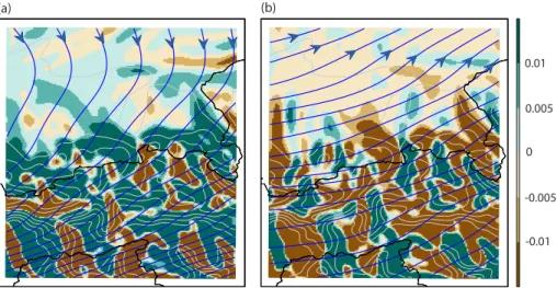
Figure 3 illustrates examples of the wind-aligned gradientG_wobtained for two circula-tion types of the PCACA9 classificacircula-tion. The marked change ofG_wacross topographic

5

crests (and across valleys) is evident, as well as its distinct spatial distribution between the two circulation types with their distinct sea level pressure gradient (geostrophic wind) over the domain.

Consideration ofG_was a candidate predictor is obviously motivated by ideas of up-slope orographic rainfall enhancement and rain shadowing on the lee of mountains.

10

Indeed at the scale of the entire ridge such flow related precipitation anomalies are clearly evident with the PCACA9 circulation type classification, at least in autumn, win-ter and spring (see Schiemann and Frei, 2010).

Apart fromG_w as defined in Eq. (3) we have also experimented with an alternative definition that has omitted the normalisation of the geostrophic wind. Such a predictor

15

was previously considered in Johansson and Chen (2003) and in Kyriakidis et al. (2001) for example. However, our experiments showed less explanatory power for precipitation in our study domain compared toG_was defined in Eq. (3). In the following, we consider

G_w simply as an alternative to the topographic gradients along the two cardinal axes and will examine how this replacement (together with the stratification of circulation

20

types) aﬀ_{ects interpolation quality for seasonal mean precipitation in the domain.}

3.3 Interpolation of daily precipitation

Our experiments on the interpolation of daily precipitation are also making use of the concepts of kriging with external drift and ordinary kriging (Sect. 3.1) as used for the in-terpolation of seasonal mean precipitation. However, rather than using the topographic

25

(17)

HESSD

11, 4639–4694, 2014

Title Page

Tables Figures

◭ ◮

Back Close

Full Screen / Esc

Discussion

P

a

per

|

D

iscussion

P

a

per

|

Discussion

P

a

per

|

Discuss

ion

P

a

per

|

topographic eﬀ_{ects are di}ﬃ_{cult to estimate. The solution followed here is to inject this}

information via pre-calculated long-term averages. The approach is somewhat related to the common use of climatological mean fields as reference (e.g. New et al., 2000; Widmann and Bretherton, 2000), but instead of adopting the reference as scaling fac-tor, uses it as trend variable in KED.

5

Following the main focus of our study on precipitation topography relationships, we conduct experiments with daily interpolations and shed light on the role of the clima-tological reference fields. To this end the interpolation errors are compared between diﬀ_{erent specifications of the trend variable (see Table 2 for a list of experiments). The}

trend settings include (a) a long-term seasonal mean built with topographic predictors

10

(experiment KED(KED1e)), (b) the long-term mean of the day’s pertinent circulation type (experiment KED(KED1e+_{)), and (c) a representation of the seasonal climatology}

that has not used topographic predictors (KED(OK)). Comparison of these settings with an ordinary kriging based direct interpolation (experiment OK(·)) will clear up the benefit of using climatological reference fields in daily interpolation.

15

Finally, we compare the results obtained in this study using KED over a small cross-section of the Alps with results obtained from a previously developed deterministic in-terpolation scheme that was applied for daily precipitation over the entire Alpine ridge (Isotta et al., 2013). The trans-Alpine method builds on a version of PRISM (Daly et al., 1994, 2002; Schwarb, 2001) for monthly long-term mean fields and on SYMAP (Frei

20

et al., 1998; Shepard, 1984) for the daily relative anomalies from the mean. The exper-iment will be denoted as SYMAP(PRISM). Results from this method rely on a cross-validation table previously calculated and provided by Isotta et al. (2013).

3.4 Evaluation

Our comparison and discussion of the various interpolation experiments is based on

25

(18)

HESSD

11, 4639–4694, 2014

Title Page

Tables Figures

◭ ◮

Back Close

Full Screen / Esc

Discussion

P

a

per

|

D

iscussion

P

a

per

|

Discussion

P

a

per

|

Discuss

ion

P

a

per

|

Two error scores will be used to summarize the performance of the methods. The first is a measure of the relative bias and corresponds to the ratio of predicted (pred_i) over observed obsi precipitation totals, averaged over all (or a subset ofn) rain gauges:

Bias=

Pn

i=₁predi

Pn

i=₁obsi

. (4)

5

The second score is defined as:

rel.MRTE=

1

n

Pn

i=₁

_p

pred_i−pobs_i2

1

n

Pn

i=₁

q

obs−pobsi

!2. (5)

Here obs is the spatial average of the observations over all (or a subset ofn) stations. The numerator represents a sort of mean squared error, but with square-root

trans-10

formed data. The transformation is introduced here to avoid excessive dependence on large precipitation values and hence to obtain a more balanced sensitivity on er-rors across the frequency distribution. The denominator is then representing some sort of spatial variance of the transformed values and this is used as a reference against which errors of the prediction are measured. Values of rel.MRTE are always greater

15

than zero. Values smaller than 1 mean that typical errors are smaller than the spatial variations. Values larger than one mean that the prediction has larger errors compared to a simple prediction of the spatial mean and this can be considered a non-skillful prediction.

Depending on the data stratification and interpolation method, between 317 and 420

20

(19)

HESSD

11, 4639–4694, 2014

Title Page

Tables Figures

◭ ◮

Back Close

Full Screen / Esc

Discussion

P

a

per

|

D

iscussion

P

a

per

|

Discussion

P

a

per

|

Discuss

ion

P

a

per

|

4 Results

4.1 Interpolation of mean precipitation

Linear regression is often considered an exploratory framework with which potential predictors for a trend model of KED can be compared. We therefore develop our dis-cussion starting with results from the special case when spatial autocorrelation is

ne-5

glected and then pursue the changes when introducing autocorrelation in combination with topographic predictors.

The number of possible regression models with three variables (elevation, north-south gradient, east-west gradient) and six diﬀ_{erent spatial scales is very large. We}

have selected three of them for our discussion because of their illustrative purposes.

10

The simplest (LM1e, see Table 1) has only elevation at the finest spatial scale (1 km) as predictor. It is a traditional and wide spread model of topography eﬀ_{ects on precipitation}

(see Sect. 1). The second (LM3e, see Table 1) involves also elevation only, but at three diﬀ_{erent space scales (75, 25, 1 km). The third model (LM9eg, see Table 1) involves}

el-evation and gradients (in both cardinal directions), again at the three space scales (75,

15

25, 1 km). Experiments with all five space scales (including also 5 and 10 km) showed that the three selected scales led to the largest values in adjustedR2. There were slight variations in the “optimal” model choice between seasons but the prescription of the three scales did not significantly lower the explanatory power. Note that a formal and automated model selection procedure (using step-wise linear regression) was not

fea-20

sible in our application, because the predictors for one scale depend on those retained for other scales (elimination of co-linearity, see Sect. 3b).

Table 3 lists values of adjusted R2 for the three selected regression models. The overall pattern is very similar between the seasons. Topography at the finest scale only (LM1e) explains a very low proportion of the spatial variance in the observations. This is

25

(20)

HESSD

11, 4639–4694, 2014

Title Page

Tables Figures

◭ ◮

Back Close

Full Screen / Esc

Discussion

P

a

per

|

D

iscussion

P

a

per

|

Discussion

P

a

per

|

Discuss

ion

P

a

per

|

not much diﬀ_{erent). Local elevation does, obviously, not explain this larger-scale pattern}

well. The situation improves when involving elevation at three space scales (1, 25 and 75 km): LM3e explains a considerable portion the precipitation variability across the domain. Finally, the largest explained variance is obtained when topographic gradient fields are included (LM9eg). Now, the predictor set involves a large-scale pattern (the

5

north-south gradient at the coarsest scale) that distinguishes between flatland, foothills and inner Alps, i.e. the major large-scale contrasts in the precipitation field that was a major obstacle for the previous two models. Interestingly, the coeﬃ_{cient (and}

statis-tical significance) of the 1 km elevation predictor is much larger in this comprehensive model than in the simple model LM1e. This suggests that there is some dependence

10

on local elevation in the distribution, but this was diﬃ_{cult to represent in the}

elevation-only models because it is superimposed by a larger-scale north-south profile that is, itself, poorly explained by elevation.

Despite its decent values in explained variance, the 9-predictor model LM9eg shows elementary deficiencies in reproducing the distribution of rain-gauge measurements in

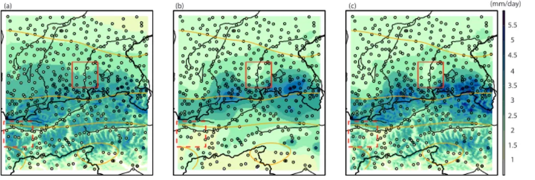
15

the domain. These are illustrated for the example of DJF mean precipitation in Fig. 4a. Precipitation is systematically overestimated over a wide flatland belt adjacent to the ridge (see e.g. full red square), underestimated along the foothills and, again, over-estimated in interior parts of the ridge (see e.g. dashed red square). Apparently, the larger-scale topographic predictors provide, in linear combination, only a partial match

20

to the observed north-south profile and the resulting prediction tends to smooth out some of the variations. Similar types of deficiencies (although diﬀ_{ering in exact}

loca-tion) were evident with other combinations or the full set of space scales, and for the other seasons. There was always clear spatial clustering in the prediction errors (re-gression residuals). It seems that, even with quite comprehensive predictor sets, it is

25

diﬃ_{cult to capture in a regression model all aspects of the precipitation field resolved}

(21)

HESSD

11, 4639–4694, 2014

Title Page

Tables Figures

◭ ◮

Back Close

Full Screen / Esc

Discussion

P

a

per

|

D

iscussion

P

a

per

|

Discussion

P

a

per

|

Discuss

ion

P

a

per

|

Ordinary kriging (OK) seeks to represent the precipitation distribution entirely without topographic predictors. The corresponding estimation (Fig. 4b) has a smooth appear-ance but reproduces the characteristic north-south contrasts between flatland, foothills and inner Alps. Hence, OK amends some of the regional deficiencies of the linear re-gression model of Fig. 4a (see red squares). However, in the inner Alpine region,

sev-5

eral rain-gauges with anomalously wet conditions (mostly at mountain peak stations) are represented as isolated spots. It appears as if some elevation dependency that is not explicitly resolved by the station network is missed out because of the absence of predictors in OK.

Figure 4c depicts the result obtained with KED, i.e. integrating predictors and spatial

10

autocorrelation, using the comprehensive three-scale elevation and gradients model as trend (KED9eg). The distribution shows the superposition of a spatially smooth pattern (similar to OK, Fig. 4b) and a small-scale pattern with topographic features that are not explicitly resolved by the station network (similar to LM9eg). The consideration of spatial autocorrelation has amended for the deficiencies of LM9eg in representing

15

the larger-scale north-south profile (e.g. red squares). Moreover, the strong contrasts between mountain stations (moist) and valley stations (dry) in the interior Alps are now integrated via an elevation (and gradient) dependence at small scales.

It is interesting to realize that the three just discussed interpolation methods yield markedly diﬀ_{erent estimates, not just regionally, but also when aggregated over larger}

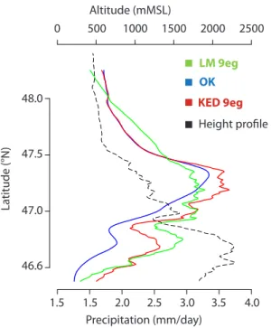
20

scales. This is further illustrated in Fig. 5, which depicts the results of Fig. 4 when averaged over latitude bands (along the ridge). OK and KED9eg both represent a moist anomaly at the foothills, centered at an elevation of about 1200 mMSL. This anomaly is much less pronounced and more wide-spread in LM9eg. Towards the inner Alpine region the three methods yield markedly diﬀ_{erent areal estimates with OK being much}

25

dryer than the regression model and KED. OK and KED diﬀ_{er by between 5–25 % in}

(22)

HESSD

11, 4639–4694, 2014

Title Page

Tables Figures

◭ ◮

Back Close

Full Screen / Esc

Discussion

P

a

per

|

D

iscussion

P

a

per

|

Discussion

P

a

per

|

Discuss

ion

P

a

per

|

high-elevation areas. But there is also a risk that KED suﬀ_{ers from overestimates, if, for}

example, the elevation dependence estimated over the full domain is not representative for the inner Alps.

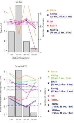
In the following we assess the relative performance of a range of interpolation mod-els from the above three categories by means of a systematic leave-one-out

cross-5

validation. Results are depicted for DJF mean precipitation in Fig. 6. The two panels are for Bias (panel a, ratio) and for rel.MRTE (panel b, dimensionless, see Sect. 3.4 for the definition of the scores). To better visualize the eﬀ_{ects of the various interpolation}

schemes, both error scores are calculated separately for the stations within four eleva-tion ranges. Here, we discuss the results more extensively for the case of DJF mean

10

precipitation, but very similar results – and similar interpretations – were found for the other seasons. This is supported by Tables 4 and 5, which list a summary of the error scores for all seasons.

When averaged over all stations the values of bias are small, varying between 0.97– 0.995 depending on method (Fig. 6a, dashed lines). The largest underestimate (three

15

percent) is obtained for LM1e (the linear model with local elevation as single predic-tor). More significant biases are, however, found in individual elevation ranges. This is particularly so for the linear regression model LM1e and for ordinary kriging OK. The lack of topographic predictors in OK impinges upon the interpolation at high elevation. Here OK systematically underestimates by about 30 %. This deficiency is mostly

cor-20

rected with interpolation models that incorporate topographic predictors (LM9eg and KED9eg). The explicit modeling of topography allows for a compensation of the eﬀ_ects

of non-representative vertical distribution of the station sample. In the framework of KED, this remedy is almost as good with only one predictor (KED1e) as with many predictors (KED9eg). In the linear model framework, however, in-situ elevation alone

25

provides a poor model of the spatial distribution (see also Table 3), and this reflects in large and alternating biases between the elevation ranges. An interpretation of this diﬀ_{erence may be seen in the fact that the estimated coe}ﬃ_{cient for the 1 km elevation}

(23)

HESSD

11, 4639–4694, 2014

Title Page

Tables Figures

◭ ◮

Back Close

Full Screen / Esc

Discussion

P

a

per

|

D

iscussion

P

a

per

|

Discussion

P

a

per

|

Discuss

ion

P

a

per

|

of spatial autocorrelation in KED1e permitted for a much more realistic separation be-tween small-scale elevation dependence (modelled by the predictor) and larger-scale precipitation variations (modelled by the autocorrelation part). In contrast, LM1e at-tempts to capture larger-scale and small-scale variations with one single linear depen-dence by construction. It is then likely that larger-scale variations (such as the

north-5

south profile) disturb a realistic estimate of the small-scale elevation dependence. The limited accuracy of linear regression models in predicting the spatial variations of seasonal mean precipitation is most evident in the relative error score rel.MRTE (Fig. 6b, Table 5). Values are close to the critical value of 1, where prediction errors are comparable to the magnitude of spatial variations (see Sect. 3.4). There is improvement

10

when including more predictors (e.g. LM9eg vs. LM1e), but considerable errors remain even with comprehensive predictor sets. This reflects results previously seen in Fig. 4a. Note, that the inclusion of the gradient at the 75 km scale (the largest considered) yields the smallest errors. Obviously, this predictor is essential for a regression model to capture the characteristic north-south profile.

15

The OK model (no topographic predictors) has much smaller errors than the regres-sion models, except for the highest elevation range (Fig. 6b). OK profits from its explicit account for spatial autocorrelation, which permits the reproduction of larger-scale vari-ations (e.g. the north-south profile) from the information at neighboring stvari-ations (see also Fig. 4b). In our application, this methodological feature yields considerably smaller

20

errors than a comprehensive predictor set in a regression model, at least for low and intermediate elevation ranges. At large elevations, however, the OK model suﬀ_{ers large}

rel.MRTE values (close to 1), which reflects the large bias there (see also Fig. 6a) and the poor reproduction of wet conditions at inner-Alpine mountain stations (see also Fig. 4b).

25

(24)

HESSD

11, 4639–4694, 2014

Title Page

Tables Figures

◭ ◮

Back Close

Full Screen / Esc

Discussion

P

a

per

|

D

iscussion

P

a

per

|

Discussion

P

a

per

|

Discuss

ion

P

a

per

|

seems to be central for reducing the caveats of OK in the inner-Alpine region (biases and over-smoothing of small-scale variations, see also Fig. 4). But the KED models also yield markedly smaller errors (at all elevations) compared to using the predictors in a linear regression.

Between the diﬀ_{erent KED models (with di}ﬀ_{erent predictor sets) there are only}

5

marginal diﬀ_{erences in the scores (Fig. 6b, Table 5). Values of rel.MRTE are roughly}

the same for the model with only one predictor (elevation at the 1 km scale, KED1e) and models with elaborate predictor sets (e.g. KED3e, KED9eg). At first sight this is surprising, given that the scores for linear regression models showed to be sensitive to the predictor sets. Our explanation of this result is that the role of topographic predictors

10

is distinct between linear models and KED. Linear models are in need of geographic predictors to capture the full distribution. The 25 and 75 km predictors are therefore highly relevant. In KED, however, the part of the distribution that is well resolved by the station network can be represented by the spatial autocorrelation component (krig-ing) and topographic predictors are primarily used to describe smaller-scale variations

15

not explicitly resolved by the station network. Here the 25 and 75 km predictors may be virtually unnecessary. The distinct role of topographic predictors in the two model families also reflects in diﬀ_{erences in the statistical significance and quantitative values}

of the predictor coeﬃ_{cients (}_β_k_{, see Eq. 1). In all the KED models, the 1 km elevation}

predictor is by far the most statistically significant, whereas in the linear models other

20

predictors (notably the 75 km topography gradient) are occasionally more significant. Experiment KED9eg (10, 5, 1 km) involves predictors at spatial scales all smaller than the station spacing. Still there seems to be little added value compared to the model with the 1 km elevation predictor only (KED1e, see Fig. 6b and Table 5). It is unclear if this result implies that the additional predictors (5 and 10 km elevations and

25

gradients) are, indeed, not very relevant (on top of the 1 km elevation) for describing small-scale precipitation variations in the Alps. There may be insuﬃ_{cient sampling of}

(25)

HESSD

11, 4639–4694, 2014

Title Page

Tables Figures

◭ ◮

Back Close

Full Screen / Esc

Discussion

P

a

per

|

D

iscussion

P

a

per

|

Discussion

P

a

per

|

Discuss

ion

P

a

per

|

Note that rel.MRTE shows a general U-shape for the more skillful interpolation mod-els (Fig. 6b), implying that relative errors are larger (smaller) at low and high (interme-diate) elevations. This pattern is also related to the definition of the score, which uses spatial variance within the elevation classes as a reference (see denominator in Eq. 3). Larger values of rel.MRTE at low elevations are primarily because of the small variance

5

in precipitation measurements over the flatland. In fact the numerator of rel.MRTE in-creases monotonically with elevation.

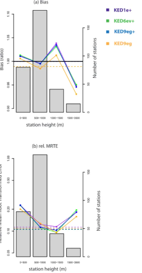
4.2 Stratification by circulation types

In this section we examine the potential of considering circulation types for the deriva-tion of interpolated mean seasonal precipitaderiva-tion fields. Two extensions will be

consid-10

ered. The first deals with a sub-stratification of the season. For this purpose, several KED interpolation models are adopted for each class of the circulation classification, separately. The resulting fields of mean precipitation for each class are subsequently re-combined into a seasonal mean field by weighting according to the classes’ fre-quency. Experiments adopting this sub-stratification are labeled with a “+_{” sign (see}

15

Table 1). The second extension deals with the circulation-dependent predictorG_w as outlined in Sect. 3.2. The wind-aligned gradient is considered here as an alternative for the gradients in the two cardinal directions. The experiment involving this topographic predictor is labeled with the letter “v” (KED6ev+_{, see Table 1). KED6ev}+ _{uses three}

diﬀ_{erent components of the} _G

w field, corresponding to three space scales (1, 25 and

20

75 km). These were derived by the smoothing procedure and removal of co-linearities, just as with the previous predictor fields (see Sect. 3b). Our results were derived with the 9-class PCACA9 classification as described in Sect. 2.

Cross-validation results with these experiments are depicted in Fig. 7, again for Bias and rel.MRTE, using the same format as in Fig. 6. Note that these are scores for

25

(26)

HESSD

11, 4639–4694, 2014

Title Page

Tables Figures

◭ ◮

Back Close

Full Screen / Esc

Discussion

P

a

per

|

D

iscussion

P

a

per

|

Discussion

P

a

per

|

Discuss

ion

P

a

per

|

of seasonal means using the previously adopted model KED9eg. Results of the two scores for other seasons are listed in Tables 6 and 7.

With all tested interpolation methods, the biases are smaller than 2 % (5 %) below (above) 1000 mMSL (Fig. 7a). The interpolation with circulation classes (KED1e+_,

KED6ev+_{, KED9eg}+_{) exhibits a slightly di}ﬀ_{erent bias pattern compared to that of}

sea-5

sonal the means directly (KED9eg), with a smaller underestimation at elevations be-tween 1500–3500 m and a larger overestimation bebe-tween 1000–1500 m. But these dif-ferences (and the bias values themselves) are small, much smaller than typical random errors, and there is not much meaning in using them for a relative assessment of the methods. The conclusion is that stratification by circulation class and usage of a

wind-10

aligned gradient G_w do not significantly change the bias pattern of the interpolation methods.

Comparison of the diﬀ_{erent methods in terms of rel.MRTE (Fig. 7b) reveals that all}

interpolation methods have a very similar error pattern. Neither the stratification by cir-culation class alone (with conventional predictors, KED1e+ _{and KED9eg}+_{), nor the}

15

consideration of a wind-aligned gradient (KED6ev+_{) can significantly improve over the}

interpolation of mean seasonal values (KED9eg). The overall scores (dashed lines) are slightly better for the stratification methods with gradient (KED9eg+_{) and wind-aligned}

gradient (KED6ev+_{) predictors (see also Table 7), but the direct seasonal method}

(KED9eg) is superior at three of the four elevation classes.

20

We have tested several alternative definitions of a circulation dependent predictor, deviating from that in Eq. (3). These included the introduction of an asymmetry between upslope and downslope gradients, truncating theG_wfield to only measure upslope gra-dients, including the wind speed (i.e. discarding the denominator in Eq. 3), and a simple model for an ageostrophic wind component. None of these alternative definitions led to

25

significantly diﬀ_{erent results.}