Adv. Geosci., 17, 1–4, 2008 www.adv-geosci.net/17/1/2008/
© Author(s) 2008. This work is distributed under the Creative Commons Attribution 3.0 License.
Advances in
Geosciences
Numerical study of two-dimensional moist symmetric instability
M. Fantini and P. Malguzzi
ISAC-CNR, via Gobetti 101, 40129 Bologna, Italy
Received: 15 October 2007 – Revised: 7 March 2008 – Accepted: 15 May 2008 – Published: 20 June 2008
Abstract. The 2-D version of the non-hydrostatic fully com-pressible model MOLOCH developed at ISAC-CNR was used in idealized set-up to study the start-up and finite am-plitude evolution of symmetric instability. The unstable basic state was designed by numerical integration of the equation which defines saturated equivalent potential vorticityq∗
e. We
present the structure and growth rates of the linear modes both for a supersaturated initial state (“super”-linear mode) and for a saturated one (“pseudo”-linear mode) and the mod-ifications induced on the base state by their finite amplitude evolution.
1 Introduction
In ordinary, stably stratified, atmospheric conditions the field of potential temperatureθ increases with height. If for any reason (e.g. a warm bubble) the vertical gradient changes sign, convective instability arises. The same principle can be formally stated for inertial instability in the horizontal direc-tion by defining an angular momentum funcdirec-tionM=v+f0x, wherev is the geostrophic wind, supposed locally parallel, andx an horizontal coordinate across the wind, with arbi-trary origin.
If we consider the two fields together, as we are bound to do, as they are in thermal wind balance, instability can take place even when the two fields,θandM, are separately stable. This happens in the presence of a horizontal thermal gradient, and its associated vertical shear of the wind. If the slope of isentropic surfaces becomes steeper than the slope of angular momentum surfaces, i.e. if
dz dx
θ=const
≡ −∂θ/∂x
∂θ/∂z > dz dx
M=const
≡ −∂M/∂x
∂M/∂z (1) then unstable motion can occur.
It is easily seen that the above condition can be written
J (M, θ ) <0 (2)
Correspondence to: M. Fantini ([email protected])
for instability. In two dimensions this can also be expressed as the requirement that potential vorticity is negative:q<0.
The above considerations hold for dry air. If moisture is to be considered, one can simply replace potential tempera-tureθwith the saturated equivalent potential temperatureθ∗
e.
Then, if the air is saturated, an atmosphere with
qe∗=J M, θe∗<0 (3)
is unstable to infinitesimal perturbations (linear instability). If the air is sub-saturated, one will need a finite amplitude perturbation to lift air to its saturation level (conditional in-stability). Symmetric instability is often referred to as slant-wise convection, although studies of the energy conversion mechanism usually conclude that the release of gravitational potential energy does not play a major role in its development (e.g. Thorpe and Rotunno, 1989).
A complete list of references on the instability, either dry or moist, infinitesimal or finite amplitude, can be found in the review by Schultz and Schumacher (1999). As far as mete-orological applications are concerned, symmetric instability is often invoked as a mechanism for the formation of frontal rainbands (e.g., Bennetts and Hoskins, 1979). An unrelated phenomenon for which symmetric instability should be re-sponsible is the appearance of areas of zero equivalent poten-tial vorticity (i.e. neutral to symmetric instability) in the core of severe midlatitude storms – often referred to as slantwise convective adjustment (see Emanuel, 1988; Kuo and Reed, 1988). Finally the matter of parameterization of slantwise convection in numerical models was examined by Nordeng (1987) and Lindstrom and Nordeng (1992) with seemingly good effects on the overall simulation of convection and pre-cipitation.
2 Model
The model we use for this study is a 2-D version of the non-hydrostatic fully compressible model MOLOCH, designed at ISAC-CNR in recent years. The main characteristics of this simplified version are that it integrates the fully compress-ible set of equations, using as prognostic variables pressure,
2 M. Fantini and P. Malguzzi: Two-dimensional non-hydrostatic symmetric instability
Fig. 1. Potential temperatureθ(color and thin contours every 10 K) and meridional windv(thick contours every 10 m s−1) for the basic
state designed for this study (see Sect. 3). The horizontal domain is covered by 1200 grid points, for a resolution of approximately 2.2 km.
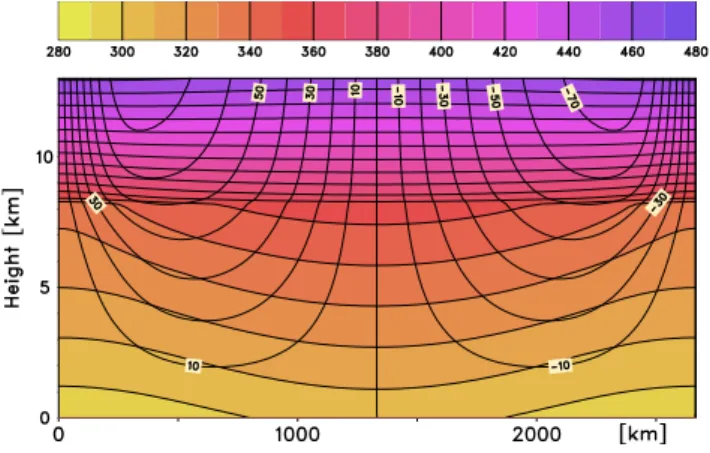
Fig. 2. Saturated equivalent potential temperatureθ∗
e (color and
thin contours every 10 K) and angular momentumM (thick con-tours every 20 m s−1). The origin is arbitrary and here chosen for
symmetry. At the bottom is the horizontal profile of saturated equiv-alent potential vorticity as from Eq. (7), which is used to design the base state up to the tropopause (see text) .
temperature, specific humidity, horizontal and vertical veloc-ity components, and five water species. Model dynamics are integrated in time with an implicit scheme for the ver-tical propagation of sound waves, while explicit, time-split schemes are implemented for the remaining terms. Advec-tion is computed using the Eulerian WAF scheme (Billet and Toro, 1997). The vertical grid is stretched exponentially with height.
Horizontal fourth order diffusion and divergence damping are included to prevent energy accumulation on the shorter
space scales. The physical scheme of the simplified version consists of only microphysics, based on the parameterisation proposed by Drofa and Malguzzi (2004). The physical pro-cesses determining the time tendency of specific humidity, cloud water/ice and precipitating water/ice are divided into ”fast” and ”slow” ones. Fast processes involve transforma-tions between specific humidity and cloud quantities, while slow ones involve rain/snow/hail production and fall. Tem-perature is updated by imposing exact enthalpy conservation at constant pressure. Fall of precipitation is computed with the stable and dispersive backward-upstream scheme, with fall velocities depending on concentration.
A fuller description of MOLOCH can be found in Mal-guzzi et al. (2006).
3 Basic state
The definition of saturated equivalent potential vorticity Q=−θex∗vz+(vx+f0) θez∗
α (4)
(notice that the non-hydrostatic contributions to relative vor-ticitywx andwydisappear in the two-dimensional version,
while the compressibility effects remain in the specific vol-umeα) was used as an equation for the vertical derivative of θ∗
e.
Starting from an imposed temperature profile at the sur-faceT=T (x)atz=0 and a uniform pressurep=p0we define pressure at the next upward level by integration of the hydro-static relation. Then the wind at the upper level is known by the geostrophic relation so that (4) can be used to findθ∗
e at
the next level upward. At this point the definitions of equiva-lent saturated potential temperatureθ∗
e and saturation mixing
ratioqVsat
θe∗=θe∗ θ (T , p) , qVsat(T , p) (5) are inverted numerically, with a simple Newton iteration, to find temperatureT
This procedure is repeated for a chosen negativeQ, and with an extremely high vertical resolution (of the order of a few meters), upward to a predefined “tropopause” level, after which a very stable stratification is imposed.
Figures 1 and 2 show the base state adopted for the ex-periment that will be discussed in the next section. It was generated with the above procedure starting from a surface temperature
T (x)=T0+(1T )
(1−cos(x))
2 (6)
with T0=293.15 K (this is the temperature at the western boundary) and1T=10 K (this is the thermal gradient over half the domain – each half of the domain is the mirror im-age of the other one, so that we were able to use periodic boundary conditions in the numerical integration).
M. Fantini and P. Malguzzi: Two-dimensional non-hydrostatic symmetric instability 3
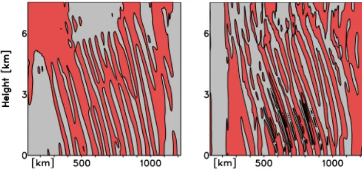
Fig. 3. Left: Vertical velocity componentw(color: grayw<0, red
w>0; contours every 1.0 cm s−1) at 17 h after initialization, on a
subdomain of Fig. 1. Right: Same except at 26 h.
Fig. 4. Left: Vertical velocity componentw(color: grayw<0, red
w>0; contours every 2.0 cm s−1at 33 h after initialization. Right:
Saturated equivalent potential temperatureθe∗(color and thin con-tours every 10 K) and absolute momentumM=v+f0x(thick
con-tours every 10 m s−1) at 33 h.
A horizontal modulation ofQwas also imposed, to con-fine the instability and avoid the occurrence of convective instability.
Q(x)=QMIN
(1−cos(2x))
2 (7)
with QMIN= − 0.25 PV units (1 PVU is equivalent to 10−6MKS units).
4 Reference experiment
We present here one run of the model, which was started with random noise of very small amplitude, and the most unstable perturbation developing was followed up to finite amplitude, when it is able to modify the base state. In order to show in one run all the features we discovered in the evolution of this form of instability, we included an artificial amount of liquid water in the initial condition (two percent of supersaturation). In other words the domain is filled by a dense cloud, in which environment the symmetric instability develops.
Figure 3 shows perturbation fields ofuandw at 17 and 26 h after initialization. Only about half of the domain, on the
Fig. 5. Same as Fig. 4 except at 40 h.wcontours every 10 cm s−1.
At this stage it can be seen how upright convection crosses vertically theMcontours instead of nearly following them as in the previous figure.
left of the center of Figs. 1 and 2, is shown. At 17 h the most unstable mode is seen to have a roughly sinusoidal structure roughly aligned with theMsurfaces. This is due to the nearly perfect symmetry of upward and downward motions in this “cloudy” environment. While the updrafts are accelerated by release of latent heat the downdrafts are equally accelerated by reevaporation of the liquid water present in the environ-ment. This is a linear stage of the perturbation (what we call “super”-linear), which is of small amplitude, sinusoidal, and grows exponentially (also see Fig. 6 below).
After a while (Fig. 3 right panel) the reevaporating down-drafts exhaust all the liquid water present in the initial cloud, and the perturbation is beginning to assume the aspect of the “pseudo”-linear mode, with updrafts becoming stronger than downdrafts. At this stage the perturbation is still small am-plitude, and grows exponentially, but does not possess all the properties that define a linear mode, in particular there is no superposition principle for these solutions.
Later on (Fig. 4) the “pseudo”-linear mode has completely taken over, and has grown to an amplitude at which it induces a visible modification on the base state. From theθ∗
e,Mplot
(Fig. 4 right) it can be seen that the effect of the perturbation has been to move warm air aloft, and that in some regions in mid-troposphere the vertical gradient ofθ∗
e changes sign.
This is a situation unstable to vertical convection, and indeed (Fig. 5) this develops, on a faster time scale than the symmet-ric one.
Figure 6 displays the growth rate computed every hour during the run, where the two distinct exponential phases (where the growth rate is approximately a constant) are ev-ident, followed by the faster growth of upright convection, and final nonlinear decay of the perturbation.
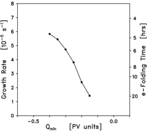
Finally, in Fig. 7, we show the growth rates of the pseudo linear mode, as determined by numerical experiments, vs the potential vorticityQMIN used in Eq. (7) to design the base state. The growth rate is computed as
σ = 1
1tlog
wMAX(t+1t ) wMAX(t )
(8)
4 M. Fantini and P. Malguzzi: Two-dimensional non-hydrostatic symmetric instability
Fig. 6. Growth rateσ of the perturbation during the reference run, as defined in Eq. (8). The dashed line marks the growth rate of the “pseudo”-linear mode (see text)
Fig. 7. Growth rate of pseudo-linear mode vsQMIN for cosine
profile as determined from the numerical model.
For a comparison with baroclinic instability consider that the maximum Eady growth rate atQ=0, which coincides with Ri=1, is 0.31f0. However, a typical Richardson number for synoptic scales is of order 100, so that a more reasonable es-timate for the growth rate of baroclinic waves in midlatitudes is an order of magnitude smaller. For the dry equivalent of Fig. 7, computed analytically, see Fig. 4 of Stone (1966).
All linear growth rates in Figs. 6 and 7 were obtained in numerical experiments initialized with random noise, and with the amplitude of the perturbation reduced every time it reached a predetermined threshold, therefore always main-taining it in the linear regime.
5 Concluding remarks
We have presented in this work a few preliminary results in regard to two dimensional non hydrostatic numerical simula-tions of symmetric instability in a saturated environment.
We have designed a basic state with prescribed negative potential vorticity, in such a way as to avoid upright
convec-tive instability while allowing symmetric instability to take place.
In this environment we have identified two types of linear instability, characterized, the first (“super”-linear) by sym-metric (up- and downdrafts) structure and higher growth rate, and the second (“pseudo”-linear) by stronger updrafts and weaker downdrafts. The “super”-linear mode was obtained by providing the initial state with enough liquid water to maintain saturation by re-evaporation in the downdraft. In the following non linear stage symmetric instability is able to trigger mid-level convection by “slantwise” advection of warmer air.
For more details on the linear stages of development see Fantini and Malguzzi (2008), where we identify and study more accurately the two types of “linear” modes, in regard to growth rates and their dependence on environmental parameters and microphysical processes.
Edited by: A. Mugnai Reviewed by: R. Rotunno
References
Bennetts, D. A. and Hoskins, B. J.: Conditional Symmetric Insta-bility – A Possible Explanation for Frontal Rainbands, Q. J. R. Meteor. Soc., 105, 945–962, 1979.
Billet, S. and Toro, E. F.: On WAF-type schemes for multidimen-sional hyperbolic conservation laws, J. Comput. Phys., 130, 1– 24, 1997.
Drofa, O. V. and Malguzzi, P.: Parameterisation of microphysical processes in a non-hydrostatic prediction model, in: Proceed-ings of 14th Intern. Conf. on Clouds and Precipitation (ICCP), Bologna, Italy, 19–23 July 2004, 1297–1300, 2004.
Emanuel, K. A.: Observational Evidence of Slantwise Convective Adjustment, Mon. Weather Rev., 116, 1805–1816, 1988 Fantini, M. and Malguzzi, P.: The slope of moist symmetric
instability with water loading, J. Atmos. Sci., 68, in press, doi:10.1175/2008JAS2695, 2008.
Lindstrom, S. S. and Nordeng, T. E.: Parameterized slantwise con-vection in a numerical model, Mon. Weather Rev., 120, 742–756, 1992.
Kuo, Y.-H. and Reed, R. J.: Numerical simulation of an explosively deepening cyclone in the Eastern Pacific, Mon. Weather Rev., 116, 2081–2105, 1988
Malguzzi, P., Grossi, G., Buzzi, A., Ranzi, R., and Buizza, R.: The 1966 “century” flood in Italy: A meteorological and hydrological revisitation, J. Geophys. Res., 111, D24106, doi:10.1029/2006JD007111, 2006.
Nordeng, T. E.: The effect of vertical and slantwise convection on the simulation of polar lows, Tellus, 39A, 354–375, 1987. Schultz, D. M. and Schumacher, P. N.: Use and Misuse of
Con-ditional Symmetric Instability, Mon. Weather Rev., 127, 2709– 2732, 1999.
Stone, P. H.: On non-geostrophic baroclinic stability, J. Atmos. Sci., 23, 390–400, 1966.
Thorpe, A. J. and Rotunno, R.: Nonlinear aspects of symmetric instability, J. Atmos. Sci., 46, 1285–1299, 1989.