equivalent with a distributed pressure field
for a FEM analysis
Daniela BARAN*, Nicolae APOSTOLESCU*
*Corresponding author
INCAS - National Institute for Aerospace Research “Elie Carafoli”
B-dul Iuliu Maniu 220, Bucharest 061126, Romania
[email protected]
Abstract: The main objective of this paper is to describe a code for calculating an equivalent system of concentrate loads for a FEM analysis. The tables from the Aerodynamic Department contain pressure field for a whole bearing surface, and integrated quantities both for the whole surface and for fixed and mobile part. Usually in a FEM analysis the external loads as concentrated loads equivalent to the distributed pressure field are introduced. These concentrated forces can also be used in static tests. Commercial codes provide solutions for this problem, but what we intend to develop is a code adapted to the user’s specific needs.
Key Words: aerodynamic loads, concentrated forces, stress analysis.
1. INTRODUCTION
The main objective of this code is to determine an equivalent system of concentrated loads for a FEM analysis. In the same time diagrams of shear forces, bending moments and torsion moments are provided for the Stress Department from the input data of the Aerodynamic Department.
The tables from The Aerodynamic Department contain pressure fields for a whole bearing surface, and integrated quantities both for the whole surface and for fixed and mobile part. Usually in a FEM analysis the external loads as concentrated loads equivalent to the distributed pressure field are introduced. These concentrated forces can also be used in static tests.
The commercial codes provide solutions for this problem, but it is useful to develop a code adapted to specific needs. ALOAD is intended to provide diagrams of the shear force, the bending moment and the torsion moment. Every aspect is intended to be solved in a friendly environment.
2. SHORT DESCRIPTION
The input data are provided by the Aerodynamic Department as input files for ALOAD. Using these values ALOAD interpolates the pressure values in given structural points (usually the intersections of ribs spars or stingers). Then these values are integrated and distributed in these structural nodes.
The principal result is a system of concentrated forces equivalent with/to the initial distribution of the pressure field – the same value of the total force and the same application point.
3. INPUT DATA
The values of the pressure field, shear force, bending and the torsion moment are collected from the Aerodynamic Department. The Stress Department provides the following data which define the finite element model: the coordinates of the structural nodes; the label (numbers) of these nodes; the links between these nodes (the finite element coverage).
The user is supposed to define whether to use a uniform mesh (and if so the user should define it), or a mesh utilized in a commercial finite element code. An example of input data is given in the following lines.
Coordinate Pressure Coordinate Pressure Coordinate Pressure
x y x y
0.40 0.00 -51.50 0.60 0.39 -177.30 0.79 0.79 -207.10 0.50 0.19 -133.70 0.69 0.59 -203.40 0.89 0.99 -214.50
… … … … … …. … … …
The interface of this stage is
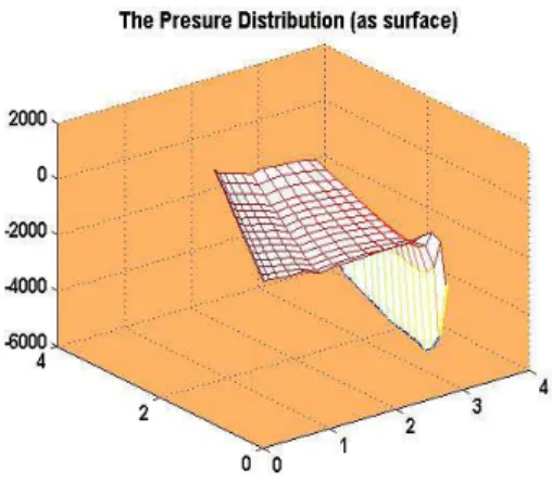
After loading the aerodynamic pressure, the next step is to visualize the aerodynamic input data. Figure 3 show an ACODE picture of the pressure distribution obtained from the above table.
Fig.2 The initial aerodynamic mesh Fig.3 The Pressure Distribution on the initial mesh
Fig. 4.The Pressure Distribution on the new mesh (here regular mesh)
Fig. 5 Aerodynamic and stress domains
4. OUTPUT DATA
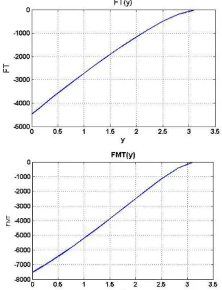
Output data are, besides the lumped forces, diagrams of the shear force, bending moment and torsion moment, obtained from the input data, and calculated from the concentrated equivalent forces. Comparing these diagrams the accuracy of the results of the ALOAD program can be evaluated.
Fig. 8 Shear force and torsion moment
Remark. ALOAD provides concentrated forces in a mesh obtained using a finite element code and/or a mesh defined by the user. Table 1 shows an example of concentrated forces required in an ANSYS analysis
Table 1. Forces (ANSYS input format) (fragment)
F ,151 ,FZ ,-16.72739 F ,152 ,FZ ,-34.0484 F ,153 ,FZ ,-35.2477
… … … …
5. METHOD
The main stages of the program are:
1) Reading the input data from the files of the Aerodynamic Department. A graphic representation of the pressure field is useful.
Using the values of the aerodynamic pressure given on the aerodynamic mesh (fig. 2 the volume on each quadrilateral element is calculated and divided between the four nodes. Then in each node of the mesh these volumes are overlapped: for an inner node there will be four numbers, for a node situated on an edge there will be two values and for a corner only one value.
In this stage we have forces in the aerodynamic mesh.
4) Then these values are interpolated in the stress mesh. (using this method the connections between the nodes of the stress model are not necessary). All the determined forces are then added and if the result is different from the aerodynamic total integrated pressure a correction factor shall be introduced.
The final result is a set of concentrated loads applied in the stress mesh with an application point near the aerodynamic point and respecting the total pressure as given by the Aerodynamic Department. Noting with ndivx and ndivy the number of divisions on Ox, respectively on Oy, the matrices X(ndivx,ndivy) and Y(ndivx,ndivy) contain the values of the coordinates of the mesh, v(ndivx,ndivy) contains the parallelepiped volumes whose bases are quadrilaterals defined by the mesh.
If we note by
v
(
i
,
j
)
the box volume whose base is the quadrilateral with the coordinates: )) , 1 ( ), , 1 ( ( )), 1 , 1 ( ), 1 , 1 ( ( )), 1 , ( ), 1 , ( ( )), , ( ), , ( ( j i Y j i X j i Y j i X j i Y j i X j i Y j i X (1)the forces in each node are calculated by the following formulas:
1
:
2
,
1
:
2
,
4
/
)
,
(
)
1
,
(
)
,
1
(
)
1
,
1
(
)
,
(
ndivy
j
ndivx
i
j
i
v
j
i
v
j
i
v
j
i
v
j
i
f
(2);
4
/
)
,
1
(
)
,
1
(
,
4
/
)
1
,
1
(
)
1
,
1
(
v
f
ndivy
v
ndivy
f
;
4
/
)
,
(
)
,
(
,
4
/
)
1
,
(
)
1
,
(
ndivx
v
ndivx
f
ndivx
ndivy
v
ndivx
ndivy
f
(3)1
:
2
;
4
/
)]
,
1
(
)
1
,
1
(
[
)
,
(
,
4
/
)]
,
1
(
)
1
,
1
(
[
)
,
1
(
ndivy
j
j
ndivx
v
j
ndivx
v
j
ndivx
f
j
v
j
v
j
f
(4)1
:
2
;
4
/
)]
1
,
(
)
1
,
1
(
[
)
,
(
,
4
/
)]
1
,
(
)
1
,
1
(
[
)
1
,
(
ndivx
i
ndivy
i
v
ndivy
i
v
ndivy
i
f
i
v
i
v
i
f
(5)
ndivx i ndivy j j i f f 1 2 ) , ( (6)6. EXAMPLES
To verify the tool, a regular mesh as the stress mesh has been generated. Now, we consider the following situations: the initial pressure field has an analytic form f(x,y)=1 and the plain domain [0,2]x[0,5].
In this case the total pressure is:
f(x,y) 10Ft (7)
and the pressure centre is:
5 . 2 ) , ( ) , ( , 1 ) , ( ) , (
dxdy y x f dxdy y x yf Y dxdy y x f dxdy y x xfXg g (8)
The resulting forces are:
) 1 1 1 1 5 . 5 . 5 . 5 . 5 . 5 . 5 . 5 . 5 . 5 . 25 . 25 . 25 . 25 . ( T F , ) 1 1 1 1 1 1 2 2 2 2 0 0 0 0 2 2 0 . 0 . ( T XF , ) 4 3 2 1 5 0 4 3 2 1 4 3 2 1 5 0 5 0 ( T YF (9)
1
18 1 18 1 . . 1
j j j j j F F XF verX
18
2
.
5
1 18 1 . . 1
j j j j j F F YF verY
(10) 10 18 1
j j F FT (11)In this case there is no difference between the total force calculated by adding the concentrated loads and that calculated by integrating the distributed force on the domain of definition.
The last example is of a horizontal empennage. Input data are presented in the aerodynamic tables with pressure values and in figures 2 and 3. The stress input data are described in table 2 containing coordinates of structural nodes and elements (connections between nodes). The concentrated forces are presented in table 2 and in table 3 we present the aerodynamic pressures. These results can be written in a text file as described in table 3.
Table 2 (fragment)
Forces and pressures in the stress mesh Node_Coordinate/1000
Node_id
x y z
Pressure Force 1 Force 2 x Af/f1
11 0.944 1.215 0.072 -192.386 -6.371 -21.91 13 1.259 1.388 0.102 -408.793 -11.554 -39.736 15 1.063 1.47 0.075 -203.629 -6.277 -21.587 17 1.37 1.657 0.105 -287.93 -10.956 -37.681 19 1.186 1.734 0.078 -209.033 -6.128 -21.075 …. …..
255 2.759 0 0.115 -2045.8 -13.343 -45.889 256 1.888 0 0.115 -144.092 -5.263 -18.1
257 0 0 0 0 -0.067 -0.231
Total F1 Total F2
-1284.23 -4416.72
Xg_Rez= 2.05
Yg_Rez= 1.49
Table 3 (fragment)
Forces and pressures in the aerodynamic mesh
Node_nr x y Pressure Force
1 0 0 0 -0.067
2 0.172 0 -20.244 -0.607
3 0.345 0 -44.74 -1.428
4 0.517 0 -63.216 -2.406
…. ….
5 0.69 0 -155.2 -4.388
267 3.215 3.094 -834.96 -12.312 268 3.327 3.094 -1378.8 -25.339 269 3.439 3.094 -4382.6 -17.485
Force = -4416.7
Xg= 2.403 Yg=1.53
7. ABOUT THE PROGRAM
ALOAD is a Visual Basic application using also MATLAB capabilities.
The Visual Basic facilities allow to create an interface for aerodynamic data and to define a new stress mesh or a set of arbitrary nodes where the lumped forces are needed. The MATLAB processor is mainly used to handle surfaces and grids in graphical representation. Also, with the MATLAB “griddata” function, based on Delaunay triangulation, we can interpolate the pressure values and the concentrated forces in the stress mesh.
The griddata form used in the application is: ZI = griddata(x,y,z,XI,YI, method). ZI fits a surface of the form z = f(x,y) to the data in the (usually) nonuniformly spaced vectors (x,y,z). “griddata” interpolates this surface at the points specified by (XI,YI) to produce ZI. The surface always passes through the data points. XI and YI usually form a uniform grid (as produced by meshgrid in our application).
The method can be one of the following:
'nearest - Nearest neighbour interpolation 'v4 - MATLAB 4 griddata method
The method defines the type of surface fit to the data. The 'cubic' and 'v4' methods produce smooth surfaces while 'linear' and 'nearest' have discontinuities in the first and zero'th derivatives, respectively. All the methods except 'v4' are based on a Delaunay triangulation of the data. In this method, a triangular mesh is formed from the control points (grid points) by connecting each point to its “natural neighbours”.
The application is developed in Windows. It can be used with Visual Basic (at least V6) and MATLAB (at least Release 13).
8. CONCLUSIONS
ALOAD provides a useful tool for any researcher or engineer interested to obtain concentrated loads for a finite element analysis from the distributed pressures. It is user friendly, allowing the analysis of many cases in a short time. It can also be used in static tests.
9. REFERENCES
[1] ANSYS 5.0[2] A. Petre, Proiectarea structurilor de aeronave si astronave, Ed. Academiei, Bucuresti, 1984. [3] G. V. Vasiliev, Bazele calculului structurilor de aviatie cu pereti subtiri, Ed. Academiei, 1998.
[4] D. Benyon, T. Green, D. Bental, Conceptual Modeling for User Interface Development, Editura Springer, ISBN 1-85233-009-0.
[5] Christopher J. Bockmann, Lars Klander, Lingyan Tang, Visual Basic, Editura Teora, ISBN 973-601-912-8. [6] Kris Jamsa, Lars Klander, Visual Basic, Editura Teora, ISBN 973-9392-48-2.