www.hydrol-earth-syst-sci.net/13/141/2009/ © Author(s) 2009. This work is distributed under the Creative Commons Attribution 3.0 License.
Earth System
Sciences
The european flood alert system EFAS – Part 2: Statistical skill
assessment of probabilistic and deterministic operational forecasts
J. C. Bartholmes1,*, J. Thielen1, M. H. Ramos1,**, and S. Gentilini1
1EC, Joint Research Centre, Institute for Environment and Sustainability, Via Fermi 2749, 21027 Ispra (VA), Italy *now at: EC, Joint Research Centre, Scientific EC Work Programme Unit, Square de Meeus 8, 1050 Brussels, Belgium **now at: CEMAGREF, Parc de Tourvoie 44, 92163 Antony Cedex, France
Received: 14 December 2007 – Published in Hydrol. Earth Syst. Sci. Discuss.: 6 February 2008 Revised: 12 January 2009 – Accepted: 12 January 2009 – Published: 5 February 2009
Abstract. Since 2005 the European Flood Alert System (EFAS) has been producing probabilistic hydrological fore-casts in pre-operational mode at the Joint Research Centre (JRC) of the European Commission. EFAS aims at increas-ing preparedness for floods in trans-national European river basins by providing medium-range deterministic and proba-bilistic flood forecasting information, from 3 to 10 days in advance, to national hydro-meteorological services.
This paper is Part 2 of a study presenting the development and skill assessment of EFAS. In Part 1, the scientific ap-proach adopted in the development of the system has been presented, as well as its basic principles and forecast prod-ucts. In the present article, two years of existing opera-tional EFAS forecasts are statistically assessed and the skill of EFAS forecasts is analysed with several skill scores. The analysis is based on the comparison of threshold exceedances between proxy-observed and forecasted discharges. Skill is assessed both with and without taking into account the per-sistence of the forecasted signal during consecutive forecasts. Skill assessment approaches are mostly adopted from me-teorology and the analysis also compares probabilistic and deterministic aspects of EFAS. Furthermore, the utility of different skill scores is discussed and their strengths and shortcomings illustrated. The analysis shows the benefit of incorporating past forecasts in the probability analysis, for medium-range forecasts, which effectively increases the skill of the forecasts.
Correspondence to:J. C. Bartholmes ([email protected])
1 Introduction
The increasing awareness that fluvial floods in Europe con-stitute a non-negligible threat to the well-being of the pop-ulation, prompted the European Commission to trigger the development of a European Flood Alert System (EFAS) in 2003. After several severe flood events of trans-national dimensions which struck Europe (EEA, 2003), the Euro-pean Commission initiated the development of a system (i.e. EFAS) that could provide medium-range pre-alerts for the trans-national river basins in Europe, and could thus raise preparedness prior to a possible upcoming flood event.
The objective of this work is to assess the skill of this specific operational hydrological forecasting system. Skill studies regarding the use of meteorological ensemble fore-casts for producing stream-flow predictions are reported in the literature (Franz et al., 2003; Clark and Hay, 2004; Roulin and Vannitsem, 2005; Bartholmes and Todini, 2005; Roulin, 2007), but none to this extent (at least to the knowledge of the authors), for systems of similar size. This makes the com-parison of skill scores obtained from the analysis of EFAS forecasts with skill scores from other studies difficult.
time period of analysis, same verification skill scores, etc.). Within the EFAS project, preliminary comparative analysis of the alert levels issued during a flood event has only been performed for individual case studies and been recently pub-lished (Kalas et al., 2008; Younis et al., 2008).
Secondly, the statistical skill assessment of EFAS forecasts here presented is unique in the sense that the scores have been calculated for the entire Europe, for each river pixel, over a period of 2 years, with a minimum of input data, and with exclusively probabilistic skill scores. Since, typically, skill scores, such as the Brier Skill Score (BSS), depend to a large degree on the chosen climatology used as reference, without having comparable input data, the comparison of skill scores from different studies remains difficult.
Part 1 (Thielen et al., 2009) of this publication focussed on the larger context within which EFAS has been developed. It presents the general and technical set-up and describes the methodologies, input data and products of EFAS. The present paper (Part 2) concerns the assessment of EFAS overall fore-casting skill over a full two-year period of existing EFAS operational hydrological forecasts.
Literature on skill scores dates back more than 120 years (Peirce, 1884; Gilbert, 1884) and often “the wheel has been reinvented” leading also to confusing double-naming of the same scores (Baldwin, 2004; Stephenson, 2000). Not all skill scores are equally suited for the skill assessment of a given forecasting system and there is no single skill score that can convey all necessary information. Therefore sets of skill scores are normally used to cover a wider spectrum of properties (Baldwin, 2004). However, care should be taken to avoid being “engulfed in an avalanche of numbers that are never used” (Gordon and Shaykewich, 2000). For the present study on EFAS skill assessment, a first set of skill measures was selected. This set was subsequently reduced further tak-ing into account the shortcomtak-ings of certain measures that arose during the analysis.
Finally, the scores used for this study are mainly described in the literature in the context of meteorological applications, but, as they deal with continuous variables that are trans-formed – using certain thresholds – into dichotomous events, it was assumed that they are as well applicable to discharge threshold exceedances as used in EFAS. The differences in terminology between hydrology and meteorology are a well known problem (see Pappenberger et al., 2008) and, where deemed appropriate, additional explanations are given in this paper.
The main reasons leading to the choice of certain skill scores are outlined in the following. The first essential aspect was that the chosen skill measures had to be equally repre-sentative for different climatic regimes that can be found over Europe. Regarding this aspect, McBride and Ebert (2000) promote the Hanssen-Kuipers skill score1 (Hanssen and
1Rediscovered Peirce (1884) skill score also referred to as True
Skill Statistic TSS (Flueck, 1987).
Kuipers, 1965) as being independent of the particular dis-tribution of observed precipitation. Similar characteristics are attributed by Stephenson (2000) to the “odds ratio”. G¨ober (2004) goes even further claiming that only the odds ratio “enables a fair comparison of categorical forecasts for different years, regions, events”. Other scores like the Criti-cal Success Index or CSI (also Thread Score / TS and Gilbert Skill Score/GSS) (Gilbert, 1884, Schaefer, 1990) or the Hei-dke (1926) skill score strongly depend on the frequency of certain (precipitation) events (Ebert and McBride, 1997). Likewise, Wilson (2001) stated that the Equitable Threat Score or ETS (Schaefer, 1990) is a “reasonable” score but that it is not independent from the observed event distribu-tion.
The second important factor considered here in the choice of skill measures was that a skill score should be as little as possible influenced by a bias in the forecast, i.e. that it should be insensitive to over- or under-forecasting. For example, Mason (1989) showed that the CSI is highly sensitive to such forecasting biases, whereas the odds ratio was found to be quite insensitive to them (Baldwin, 2004). In this context, Gandin and Murphy (1992) defined a score asequitableif random and constant forecasts result in the same score value, and if they do not encourage over- or under-forecasting as the score is maximised for unbiased forecasts (bias=1). Scores like percentage correct (PC) were found to be not equitable as they could be easily “improved” by over-forecasting. It was, however, stated by Marzban (1998) that there is no such a thing as a strictly equitable skill score when it comes to forecasting extreme events.
Some of these properties and the final choice of skill scores for this study will be discussed in Sect. 3. An extensive re-view on skill scores can be found in Stanski et al. (1989), as well as in the works of Murphy (1996, 1997).
This study looks at the past performance of a forecasting system, but also aims to improve the future performance of such a system by making it possible to incorporate the past experience into the current forecasting procedure, thereby al-lowing the forecaster to better estimate the probability of a current forecast. This is particularly important for a flood alert system that covers a heterogeneous area with several river basins and for which local expertise is not always at hand.
This paper is structured in the following way: in Sect. 2, a short description of the data used is given, followed by the description of the methodology in Sect. 3. Results are pre-sented in Sect. 4 and discussed in Section 5, followed by the final conclusions in Sect. 6.
2 Data
EUE or EPS for Ensemble Prediction System) forecasts of the European Centre for Medium-Range Weather Forecasts (ECMWF) are the input data for EFAS. The forecast ranges are 10 days for the ECMWF forecasts and 7 days for the DWD forecasts. In the absence of discharge measurements to set up the initial conditions at the beginning of the fore-casts, a proxy for observed discharge is calculated using ob-served meteorological station data that is provided by the JRC MARSSTAT Unit (internet: http://agrifish.jrc.it). The data used in EFAS are described in more detail in Part 1 (Thielen et al., 2009).
The present analysis is based on operational EFAS dis-charge forecast data simulated using the 12:00 UTC weather forecast for the full 25-month period of January 2005 to February 2007. Grid cells with upstream area of less than 4000 km2are not included in the analysis as previous works (Bartholmes et al., 2006) showed that EFAS skill computed as a function of upstream areas remains similar for areas greater than 4000 km2. EFAS skill only deteriorates when going below this threshold, which corresponds to the spatial resolution of the meteorological data that were used for the calibration of the forecasting system.
In the pre-operational system, only leadtimes of 3 to 10 days are considered, due to the medium-range pre-alert ori-entation of EFAS. It is considered that for short leadtimes dis-charges can be forecasted much better by the national hydro-meteorological services. From the technical point of view, it should also be mentioned that for leadtimes shorter than 3 days, the influence of deterministic initial conditions is still important on the probabilistic forecasts, and spread (i.e. un-certainty information) is limited. However, in this study, for completeness of the analysis and research purposes, dis-charge forecast data for all leadtimes, from 1 to 10 days, were considered.
We also note that in our first efforts to perform the skill assessment of EFAS forecasts (Bartholmes et al., 2006) se-rious shortcomings due to a lesser quantity of data available (i.e. too few forecasted events) appeared. We consider that in the present study, based on 2 years of data, the results are statistically more significant.
3 Methodology
Skill assessment in deterministic stream-flow hydrology nor-mally compares observed point measurements (discharges at gauging stations) with simulated discharges from hydrologi-cal model output. The Nash-Sutcliffe coefficient (Nash and Sutcliffe, 1970) is one of the most used skill scores in hy-drologic simulation and gives a measure of the discrepancy between observed and simulated discharges. In order to give meaningful results, this method needs good observed data for every point of interest and a single model hydrograph to compare it against. When it comes to probabilistic skill assessment of hydrologic forecasts this kind of skill score
is less useful. Even if it can be used with the mean of a hydrological probabilistic forecast (Mullusky, 2004), in this study it was decided not to adopt the Nash–Sutcliffe coeffi-cient because it does not take into account all the probabilis-tic aspects of the EFAS forecasts, and thus omits valuable information. Specifically, probabilistic forecast performance cannot be verified in the same direct way as the determin-istic one (i.e. comparison of one observed/forecasted value pair per time step). Instead, observed event frequencies have to be compared to forecasted probabilities, thus necessitating long enough time-series for a statistically meaningful evalu-ation.
In this context, methods adopted from meteorology – where probabilistic forecasts are already more commonly used – are applied here to assess the skill of EFAS opera-tional forecasts. The variables and the tools used in this anal-ysis are explained in the next paragraphs.
3.1 Variable analysed: the threshold exceedance
Analysing the performance of a hydrological forecasting sys-tem at European scale by performing the analysis of the full probabilistic distribution of discharges or a cost-benefit anal-ysis of forecasts issued by the system is not possible, as not all the required data is available at this scale. Therefore, in this analysis, EFAS forecasted discharges are not processed as continuous variables but are reduced to binary events of exceeding or not exceeding a threshold. In other words, the maps describing EFAS forecasts analysed here contain only information if a forecasted discharge in a pixel is above or below a certain threshold. To get to these thresholds, a long term simulation (1990–2004) with the EFAS hydrolog-ical model LISFLOOD (de Roo, 2000; van der Knijff and de Roo, 2006) was performed (using the same set-up as the operational system) and statistical thresholds were deduced from the simulated discharges for every grid cell. This ap-proach has the advantage that any systematic over- or under-prediction of the model is levelled out (see Part 1, Thielen et al., 2009, for more details). The two thresholds (and def-initions) that indicate a probability of flooding and thus are most important for EFAS forecasts are:
Severe EFAS alert level (SAL) threshold:
– very high possibility of flooding, potentially severe flooding expected
High EFAS alert level (HAL) threshold:
– high possibility of flooding, bankful conditions or higher expected
Table 1. Contingency table for the forecast verification of given dichotomous events.
Observed (Proxy)
YES NO
Forecasted YES a (HIT) b (FA) a+b
NO c (MISS) d (CR) c+d
a+c b+d a+b+c+d
3.2 Criterion of persistence
In a medium-range forecasting system like EFAS, a flood event is forecasted, in most cases, several days ahead of the event when it is flagged for the first time by the system. The forecaster has the possibility to adopt a “wait and see” at-titude until the next forecast(s) and only take an event into closer consideration if it is confirmed, i.e. if it is forecasted persistently. In this study, we tested if the use of a persis-tence criterion leads also to quantifiable improvements of the forecast quality.
The following definitions for persistence were used: A forecast is considered as persistent only if the alert threshold exceedance in a river pixel is forecasted continu-ously on 2 consecutive dates.
In the probabilistic EPS2-based forecasts (EUE), the per-sistence criterion is also linked to a 2nd threshold: a mini-mum number of EPS members has to be persistently above the alert threshold.
3.3 Contingency tables
Assuming that the position in time of pairs of forecast (f ) and observation (x)[(fi, xi), i=1, n] is negligible, the em-pirical relative frequency distribution of the analysed sam-ple “captures all relevant information” (Murphy and Winkler, 1987) and the joint distribution off andx can be presented by a 2×2 contingency table (see Table 1).
For the construction of contingency tables, the forecasted discharges are transformed into dichotomous events (Atger, 2001; Bradley et al., 2004) regarding the following criteria: does a discharge exceed the EFAS high alert threshold? Do at least 5, 10, 20 etc. EPS members (out of 51 members) fore-cast a discharge exceeding the EFAS high alert threshold? Is the forecast persistent?
For every combination, a contingency table was calcu-lated for each river pixel with an upstream area larger than 4000 km2. The four fields of the contingency table are illus-trated in Table 1. When the persistence criterion is applied, the event is considered as “Forecasted” if and only if it is forecasted continuously on 2 consecutive dates. For exam-ple, an event with persistence=20 EPS would be only classi-fied as “Forecasted” if the previous and the present forecasts
2Ensemble Prediction System.
Forecasted probability
Observed frequenc
y
Perfect reliability line
Forecasted probability
Observed frequenc
y
Perfect reliability line
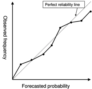
Fig. 1.Schematic reliability diagram.
had at least 20 EPS forecasting a discharge greater than the EFAS high alert threshold.
3.4 Reliability diagram
The reliability diagram (Wilks, 1995) is used to assess the “reliability” of a probabilistic forecast of binary events, i.e. it analyses how forecasted and observed event frequencies compare (see Fig. 1). The forecasted event probabilities of the EFAS EPS forecasts are plotted on the x-axis against the observed event frequencies of the proxy on the y-axis. The closer the data points in this plot are to the 1:1 diagonal line, the more reliable is the forecast. In the case of perfect relia-bility, a forecast predicting an event withX% of the ensemble members would haveX% of probability to happen.
3.5 Choice of appropriate skill scores
Taking into account the findings in the literature (see Intro-duction), the “odds ratio” and the Hanssen-Kuipers score (HK) (both equitable) were chosen as skill measures that do not make explicit use of a comparison to a benchmark forecast (Eqs. 1 and 2). As advocated in Stephenson (2000), these two measures are complemented with the Frequency Bias (FB) (Eq. 3).
Odds=ad
bc range[0,∞],best: ∞ (1)
HK= a
a+c− b
b+drange[−1,1],best:1 (2) FB= a+b
The Brier skill score (BSS) (Brier, 1950) is widely used in the skill analysis of meteorological probabilistic forecasts. In this study, it was chosen as an inherently probabilistic and strictly proper score – a score is “proper” when it is opti-mized for forecasts that correspond to the best judgement of the forecaster, and it is “strictly proper” if there is only one unique maxima (Murphy and Epstein, 1967). Furthermore, the Brier skill score is(a)a highly compressed score, as it di-rectly accounts for the forecast probabilities without necessi-tating a contingency table for each probability threshold, and (b)uses a user-defined benchmark forecast (here, the clima-tology3) (Eqs. 4 and 5):
BSS=1− BSf BSclim
range[−∞,1],best:1 (4) with
BS= 1 N
N X
1
(p−o)2range[0,1],best:0 (5)
whereprefers to the probability with which an event is fore-casted andois the binary value of the observation (o=1.0 if the event is observed ando=0.0 if it is not observed).Nis the total number of forecast dates. The underscorefdenotes the forecast that is analysed, while clim stands for climatology.
As the most intuitive scores, also the probability of detec-tion (POD, Eq. 6) as well as the frequency of hits (FOH) and frequency of misses (FOM) (Eqs. 7, 8) were chosen:
POD= a
a+crange[0,1],best:1 (6)
FOH= a
a+brange[0,1],best:1 (7)
FOM= c
a+crange[0,1],best:0 (8)
4 Results
The results obtained from the two-year skill assessment exercise (2005–2007) are presented first as absolute num-bers of the three contingency table fields: “hits”(h), “false alerts”(f ) and “misses”(m). As the analysed events (ex-ceedances of the EFAS HAL threshold) can be regarded as rare4, the fourth field (d in Table 1) – i.e. “positive reject” – is not shown, as it contains numbers roughly two magnitudes bigger than the other three fields, and is of far less interest to this analysis. Additionally, due to the very high number of combinations (and thus contingency tables) only the most representative results are shown.
3Climatology: Sample mean frequency of the event computed
using long-term statistics. Here, the historical frequency of an event to exceed the HAL threshold.
4EFAS HAL threshold is defined – for each grid cell separately
– as the discharge above the 99th percentile of ranked long term daily discharges, see also Part 1 (Thielen et al., 2009).
4.1 Positive effect of persistence
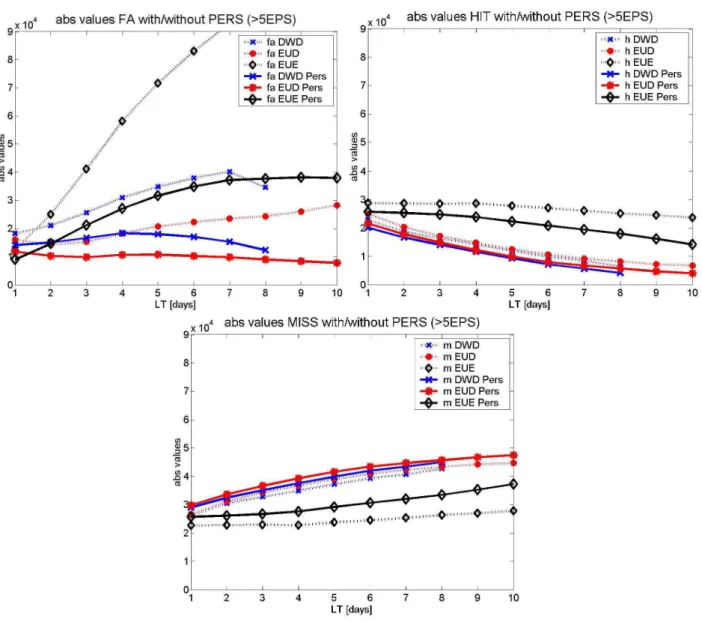
Figure 2 (top left) shows the number of false alerts (f ) as a function of leadtime for the deterministic (DWD and EUD) and probabilistic (EUE) forecasts (>5EPS, i.e. more than 5 EPS-based simulations giving discharges above EFAS HAL). The effect of using the persistence criterion (full lines) is clearly visible as the number offalse alertsis reduced by up to 70%. On the contrary, hits (h)(Fig. 2 top right) and misses(m)(Fig. 2 bottom) are far less influenced by persis-tence. Actually, the numbers ofhitsandmissesfor the deter-ministic EFAS forecasts are hardly changed at all and just for EFAS EPS (EUE) thehitsare reduced while themissesare proportionally increased. However, these changes become much less significant for higher numbers of EPS and are in-significant for forecasts with more than 15 (out of 51) EPS-based simulations above EFAS HAL.
When looking athits,false alertsandmissesfor a given leadtime, i.e., varying only the minimum number of EPS that have to exceed HAL for the event to be regarded as “Fore-casted”, the general behaviour of curves is similar to the ex-ample in Fig. 3, where the number of occurrences is plotted for a leadtime of 4 days. By increasing the minimum num-ber of EPS-based simulations forecasting discharges above the EFAS high threshold, the number offalse alertsbecomes drastically smaller, the number ofhitsbecome smaller to a much lesser extent, while the number ofmissesincrease pro-portionally to the decrease in the number ofhits.
4.1.1 Frequency of hits (FOH) and frequency of misses (FOM)
Fig. 2. Absolute numbers of “false alertsf” (top left),“hitsh” (top right) and “missesm” (bottom) for deterministic forecasts (DWD and EUD) and at least 5 EPS>HAL (EUE) over leadtime, with (full line) and without (dottetd line) persistence.
4.1.2 Frequency bias
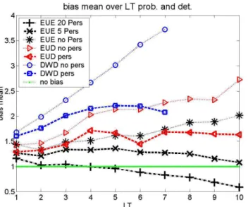
The frequency bias (FB) (Eq. 3) of EFAS forecasts is re-ported in Fig. 5. The FB values for the deterministic DWD-based forecasts are higher than the FB values for the EUD-based forecasts (ECMWF). The lowest FB results were for the probabilistic EUE-based forecasts. In general, the FB values calculated with the persistence criterion (full lines) are significantly lower than the ones calculated without taking persistence into consideration (dotted lines). Furthermore, Fig. 5 shows that there is a general tendency to over-forecast (i.e. forecast more events than the proxy-observed ones) as the bias value is greater than one. For 20 persistent EPS members, the bias is around 1 (i.e., no bias, indicated by the “bias=1” line in Fig. 5) for the first forecast days of lead-time, but it drops below 1 after day 5. For 5 persistent EPS
members, the bias stays between 1.4 and 1.1. For the de-terministic forecasts, DWD and EUD-based forecasts with persistence have bias values between 1.3 and 2.5.
4.1.3 Brier skill score
When using the Brier skill score (BSS) it has to be kept in mind that the interpretation of BSS values can be very sensitive to the choice of the reference climatology (Hamill and Jura, 2006). To check this influence on the results of the present analysis, two reference climatologies were com-pared. On the one hand, the probability of having dis-charges greater than EFAS high alert threshold (HAL) was set to Pclim= 0.00, following the suggestions of Legg and
Fig. 3. Absolute numbers reporting the three contingency table fields “hits”(h[x]), “false alerts”(f [+]) and “misses”(m[o]) for at least 5 EPS in the previous forecasts at leadtime 4 days .
which corresponds to the empirical event frequency with which the EFAS HAL thresholds (threshold discharge not ex-ceeded in 99% of the cases) were calculated. The results ob-tained for these two reference climatologies were not signif-icantly different and hence all the diagrams presented here-after show BSS usingPclim= 0.01.
Results for the BSS median values are reported in Fig. 6. The deterministic forecasts without the persistence crite-rion show no skill compared to the reference (climatology), i.e. the BSS is zero. Also, when considering persistence, they show only very little skill in the first days of leadtime. From Fig. 6, one can see that, with persistence, the Brier skill score stays around 0.0, and, without persistence, it drops steeply after some days of leadtime. The BSS values for the deter-ministic DWD- and EUD-based forecasts become negative after leadtimes of 3 days and 5 days, respectively. The BSS median for the EPS-based forecasts (EUE) shows the high-est skill when persistence is not considered and, for all lead-times, it shows higher skill than the deterministic forecasts.
Figure 7 shows the relative frequency of EPS BSS values for leadtimes 3, 6 and 10 days in bins with size 0.2: on the top, with no persistence and, on the bottom, with persistence of 20 EPS. When looking at these relative frequencies of the EPS BSS (Fig. 7), one can see that persistence increases the relative frequency of the positive BSS values in the lower skill range (BSS values smaller than 0.4). The increase in relative frequencies of the higher BSS values (0.8–1.0) in the case without persistence (Fig. 7, top) can be regarded as an artefact of the small event probability: if in a pixel nothing is observed in 2 years, but the exceedance of HAL with 1 EPS is (wrongly) forecasted 5 times in the same period, the BSS
Fig. 4. Frequency of hits (FOH) [x] and frequency of misses (FOM) [o] for deterministic persistence and 15 EPS persistent (top) and 5 and 35 EPS persistent (bottom). 1:1 line means num-ber of misses=numnum-ber of hits (for FOM) and numnum-ber of false alerts=number of hits (for FOH).
value is>0.95 for this pixel. This kind of noise is eliminated by the persistence criterion as can be clearly seen in Fig. 7 (bottom).
Fig. 5.Frequency bias over leadtime for EUD, DWD and EUE with no, 5 and 20 persistent EPS.
Fig. 6.BSS median over leadtime. For deterministic forecasts with and without persistence and for the EUE with 0, 5 and 20 persistent EPS.
0.4 for upper and lower Danube (and tributaries) and almost zero or even negative for middle Danube and Tisza (Hungar-ian tributary).
4.1.4 POD and HK
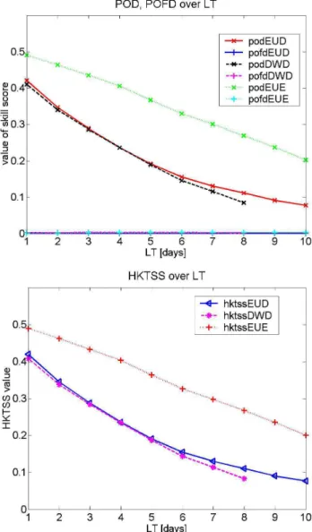
Figure 9 shows the POD (Eq. 6), the POFD (second term of HK/TSS in Eq. 2) and the Hanssen-Kuipers skill score (HK or TSS). It can be seen that the POFD is very close to zero, while the POD and the HK basically take the same val-ues. This is a consequence of the fact that for relatively rare events, like the exceedances of the EFAS HAL threshold,
Fig. 7. Relative frequency distribution of Brier skill score (BSS) values (0=no skill, 1=perfect forecast). 1 curve per leadtime. Top no persistence, bottom 20 EPS persistent.
Fig. 8.Areal distribution of BSS median values for 6 days of lead-time and persistence (>5 EPS)
A different picture is obtained for the skill expressed as odds (Fig. 10): the decrease with leadtime for EUE is steeper than that observed for the POD skill score and, with increas-ing persistence thresholds of EPS-based forecasts, the skill score yields higher (i.e. better) values.
4.2 Reliability diagram
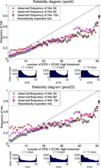
The reliability diagrams obtained from EFAS forecasts for leadtimes 3, 6 and 10 days are shown in Fig. 11. The three histograms presented below the reliability diagrams show the numbers of hits that correspond to the respective relative fre-quency in the reliability diagram for the leadtimes 3, 6 and 10 days. These histograms show that every data point in the reliability diagram is calculated with at least 250 pixels that had a hit.
It can be seen that for most EPS thresholds the results for EFAS hydrological forecasts are below the diagonal (perfect reliability), meaning that during the study period the EFAS forecasts were over-predicting – i.e. predicting a higher prob-ability than the actually observed frequency of occurrence. The probability of a hit with 51 EPS members predicting a discharge greater than EFAS HAL is only 80%, and, with 48 EPS members, it is less than 60%.
In Fig. 11, the notion of persistence in the EPS threshold refers only to the number of EPS simulations above EFAS HAL in the previous forecast, when the actual forecast has at least 1 EPS member above HAL. This choice reveals a result that would have been obscured if we had omitted the
Fig. 9.POD and POFD (top) and Hanssen-Kuipers (HKTSS) (bot-tom), for both deterministic forecasts based on EUD and DWD and for 15 persistent EPS (EUE).
results for EPS numbers smaller than the persistence thresh-old. Namely, with increasing the threshold of EPS exceeding HAL in the previous forecast, the probability to have a hit becomes higher for the lower EPS numbers, leading to the tendency to under-predict (as observed in the reliability dia-gram of Fig. 11 bottom). Actually, if the previous forecast predicted 20 EPS>HAL, the probability of a hit with 3 days leadtime is around 30%, no matter if the current forecast is 1 or 25 EPS>HAL (see lower diagram in Fig. 11).
5 Discussion
Fig. 10. Skill measures of odds over leadtime for EUD, DWD, 5 persistent EPS (top) and 25 persistent EPS (bottom).
the forecasted signal in two consecutive forecasts. The fre-quency bias is influenced positively by the persistence crite-rion and waiting for persistence of at least 5 EPS members, even results in decreasing bias over leadtime (Fig. 5). In gen-eral, the use of the persistence criterion leads to a strong de-crease offalse alerts (f). However, this comes at the cost of a moderate increase ofmisses (m), as well as a moderate de-crease ofhits (h). The probability to have ahitwith a low number of EPS is strongly increased through the use of the persistence criterion (see Fig. 11). Increasing the threshold for persistent EPS members, the skill expressed as odds in-creases, while the scores BSS, POD and HK (TSS) decrease. The odds skill score decreases with leadtime and increases for increasing EPS thresholds. The interpretation of the re-sults obtained with complex skill scores is not straightfor-ward. One should be aware of the specific behaviour of each skill score and their tendency to be strongly influenced by
Fig. 11. Reliability diagrams for the cases that the previous fore-cast had<5EPS (upper diagram), or≥20EPS (lower diagram). In each diagram 3 leadtimes (3, 6, 10 days) are reported. Points on the diagonal line have perfect reliability (i.e. forecasted probabil-ity=observed frequency). In the small histograms the absolute num-ber of hits for each EPS numnum-ber threshold that was used to create the reliability diagrams is reported.
one of the fields of the contingency table. Therefore, it is very important to look also at the absolute numbers from the contingency tables, as well as to consider simple skill mea-sures like FOH, FOM and POD that give a direct idea of the ratios between the fields of a contingency table.
than zero in all fields. Additionally, even when all fields were filled in, we often faced the fact that the number ofhits,false alerts, andmisseswas very low and, consequently, the num-ber of positive rejects was very high – i.e., in the order of two magnitudes higher thanhits,false alertsandmisses.For skill scores like the HK, this meant that it was principally reduced to the same values as the POD.
In the analysis of the deterministic forecasts, the skill of EFAS hydrological forecasts using DWD meteorological data as input was in general lower than the one obtained with ECMWF products. Other studies in the literature indicate that the DWD precipitation forecasts tend to have also lower scores than the ones from ECMWF (see for instance Pede-monte et al., 2005). In the present study, this result might be due to a scaling issue: the spatial resolution of the DWD data used in EFAS is much higher than the spatial resolution of the JRC-MARS observed meteorological data that was used to calibrate the EFAS LISFLOOD model and to define a proxy for observed discharges in the skill assessment. The spatial resolution of ECMWF data was much more similar to the resolution of the JRC-MARS data. It is expected that fore-casted precipitation intensities are higher at higher spatial resolutions and that convection in the DWD model is better resolved. Given this, it seems plausible that the EFAS dis-charges simulated with DWD data as input were sometimes too high (compared with the proxy-observed ones), resulting in a relatively higher number of false alerts, while the num-ber of hits and misses was very similar to the results based on ECMWF data. This aspect needs to be further investigated, and is beyond the scope of this paper.
In the probabilistic forecasting framework, it is of high importance for the forecaster to know the probability that a forecasted event will happen. This study shows that the as-sumed equi-probability (i.e. reliability) of predictions from EPS in meteorology – which assumes that if 5 out of 50 EPS members forecast an event, there is a 10% chance for the event to happen – is not linearly translated into the hydro-logical probabilistic forecasts issued by EFAS. There are in fact strong biases (see Sect. 4.2) between the observed and expected frequencies.
It was shown that in the case of EFAS forecasts the proba-bility of a current forecast is heavily conditioned by the prob-ability that was forecasted in the previous forecast. The use of the persistence criterion successfully incorporates this in-formation from past forecasts into the present EFAS forecast. This study aims at analyzing the past performance of EFAS forecasts regarding a proxy for observed discharges. It has no ambitions on identifying at which point (in river loca-tion, forecasting leadtime, upstream area or number of EPS-based simulations forecasting the event) there is a skill in the forecasts. Skill scores are applied to a two-year period of ex-isting operational forecasts in order to obtain a first picture of the performance of the forecasting system on a European scale. However, it must be stressed that the notion of skill and quality of a forecasting system depends heavily on the
needs and acceptable trade-offs of the end-user. For a system like EFAS, aimed at complementing local forecasts issued by different hydrological services in different countries and river basins, the role of the end-user in defining references and thresholds to be used in skill assessment studies is cru-cial. In this context, the general goal is to build skill scores that are tailored to the specific needs of the user and that will contribute to increase the utility (and economic value) of a forecast.
Additionally, it must be noted that although the “number-crunching” exercise as performed in this study tried to mimic the behaviour of the human EFAS forecaster (notably by in-troducing a persistence criterion when flagging an event as a “forecasted” one), all efforts in this regard can only be done to a certain degree. It is certainly difficult (maybe even im-possible) to translate the expertise of the forecaster into to-tally objective rules. Over the past two years, EFAS perfor-mance, in terms of success rate of external alerts sent out to national authorities whenever EFAS forecasts a potential flood situation, showed a hit rate of roughly 80%, which is much higher than what is indicated in the results of this study. Such a high performance was mainly achieved by the gaining of experience of the EFAS forecast team over time, as well as by the adoption of a more conservative attitude when send-ing out EFAS alerts, through which the number of false alerts was lowered drastically. Therefore, the results of this study should be taken as indicative of the system’s performance, and the reader should bear in mind that they have a tendency to be more pessimistic than what has been observed in the past two years.
Finally, it should be noted that the verification of forecasts against observed flood events that are spread all over Europe is quite a complicated task. At such large scale of action, any observed data (real or proxy) will hardly include all observed flood events, and the introduction of a bias from taking into account too few misses is practically inevitable.
6 Conclusions
As expected from such a global approach at a Euro-pean scale, there are significant differences in skill for different rivers. This is linked to the different hydro-meteorological conditions encountered in European trans-national river basins, but also to calibration issues (data scarcity and not equally representative in space) and varying skill in the meteorological forecast input.
Finally, the findings of this study will be incorporated into the pre-operational EFAS at a pixel basis. The aim is to give the forecaster the possibility to assess past performance of the system at any time and to give guidance to the forecaster in estimating the forecast probability of an event to happen. The first step to assign a probability to EFAS flood forecasts might come from the results indicated in the reliability dia-grams that were presented in this study. A second step will go further, with the incorporation of weather forecasts from different types (deterministic and probabilistic weather pre-dictions). The general idea is to treat the deterministic fore-casts as part of the ensemble probabilistic forecasting system by assigning them a weight and then assessing the resulting total probability of the ensemble flood forecasts.
Acknowledgement. The authors gratefully acknowledge the support of all staff of the weather driven natural hazards action and LMU IT support. The authors would also like to thank the Deutsche Wetterdienst and the European Centre for Medium-Range Weather Forecasts, as well as the JRC IPSC. Thanks go also to F. Pappenberger for fruitful brainstorming. For their financial sup-port the authors thank the European Parliament, DG Environment and DG Enterprise.
Edited by: L. Pfister
References
Atger, F.: Verification of intense precipitation forecasts from sin-gle models and ensemble prediction systems, Nonlin. Processes Geophys., 8, 401–417, 2001,
http://www.nonlin-processes-geophys.net/8/401/2001/.
Baldwin, M. E. and Kain, J. S.: Examining the sensitivity of various performance measures, 17th Conf. on Probability and Statistic in the Atmospheric Sciences, 84th AMS Annual Meeting, Seattle, WA, 2.9, 1–8 January, 2004.
Bartholmes, J. and Todini, E.: Coupling meteorological and hydro-logical models for flood forecasting, Hydrol. Earth Syst. Sci., 9, 333–346, 2005,
http://www.hydrol-earth-syst-sci.net/9/333/2005/.
Bartholmes, J., Thielen, J., and Ramos, M. H.: Quantitative analy-ses of EFAS forecasts using different verification (skill) scores, in: The benefit of probabilistic flood forecasting on European scale, edited by: Thielen, J. , EUR 22560 EN, 58–79, 2006. Bradley, A. A., Schwartz, S. S., and Hashino, T.:
Distributions-Oriented Verification of Ensemble Streamflow Predictions, J. Hydrometeorol., 5(3), 532–545, 2004.
Brier, G. W.: Verification of forecasts expressed in terms of proba-bility, Mon. Weather Rev., 78, 1–3, 1950.
Clark, M. P. and Hay, L. E.: Use of Medium-Range Numeri-cal Weather Prediction Model Output to Produce Forecasts of Streamflow, J. Hydrometeorol., 5(1), 15–32, 2004.
De Roo, A., Wesseling, C. G., and Van Deurssen, W. P. A.: Physi-cally based river basin modelling within a GIS: the LISFLOOD model, Hydrol. Process., 4(11–12), 1981–1992, 2000.
EEA, European Environment Agency: Mapping the impacts of re-cent natural disasters and technological accidents in Europe, En-vironmental issue reportNo. 35, published by European Envi-ronment Agency, Copenhagen, 2003, p. 47, 2003.
Flueck, J. A.: A study of some measures of forecast verifica-tion, Preprints, 10th Conf. on Probability and Statistics in Atmo-spheric Sciences, Edmonton, AB, Canada, Amer. Meteor. Soc., 69–73, 1987.
Franz, K. J., Hartmann, H. C., Sorooshian, S., and Bales, R.: Verifi-cation of National Weather Service Ensemble Streamflow Pre-dictions for Water Supply Forecasting in the Colorado River Basin, J. Hydrometeorol., 4(6), 1105–1118, 2003.
Gandin, L. S. and Murphy, A.: Equitable skill scores for categorical forecasts, Mon. Weather Rev., 120, 361–370, 1992.
Gilbert, G. F.: Finley’s tornado predictions, Am. Meteorol. J., 1, 166–172, 1884.
G¨ober, M., Wilson, C. A., Milton, S. F., and Stephenson, D. B.: Fairplay in the verification of operational quantitative precipita-tion forecasts, J. Hydrol., 288, 225–236, 2004.
Gordon, N. D. and Shaykewich, J. E.: Guidelines on Performance Assessment of Public Weather Services – Geneva: WMO, 2000, (WMO/TD 1023), 2000.
Hamill, T. M. and Jura, J.: Measuring forecast skill: is it real skill or is it the varying climatology?, Q. J. Roy. Meteorol. Soc., 132, 2905–2923, 2006.
Hanssen, A. W. and Kuipers, W. J. A.: On the relationship be-tween the frequency of rain and various meteorological parame-ters, Meded. Verh., 81, 2–15, 1965.
Heidke, P.: Berechnung des Erfolges und der Gute der Wind-starkevorhersagen im Sturmwarnungsdienst, Geogr. Ann., 8, 301–349, 1926.
Legg, T. P. and Mylne, K. R.: Early warnings of severe weather from ensemble forecast information, Weather and Forecasting, 19, 891–906, 2004.
Kalas, M., Ramos M. H., Thielen, J., and Babiakova, G.: Evaluation of the medium-range European flood forecasts for the March– April 2006 flood in the Morava River, J.Hydrol. Hydromech., 56(2), 116–132, 2008.
Marzban, C.: Scalar measures of performance in rare-event situa-tions, Weather and Forecasting, 13, 753–763, 1998.
Mason, I.: Dependence of the critical success index on sample climate and threshold probability, Aust. Met. Mag., 37, 75–81, 1989.
Ebert, E. and McBride, J. L.: Methods for verifying quantita-tive precipitation forecasts: application to the BRMC LAPS model 24-hour precipitation forecasts, BRMC Techniques De-velopment Report No. 2, 87 pp., 1997.
McBride, J. L. and Ebert, E.: Verification of quantitative precipi-tation forecasts from operational Numerical weather prediction models over Australia, Weather and Forecasting, 15, 103–121, 2000.
forecasts in the NWS Advanced Hydrologic Prediction Services (AHPS), AMS 16th Conference on Numerical Weather Predic-tion Symposium on Forecasting the Weather and Climate of the Atmosphere and Ocean, Seattle, Paper J11.5, 2004.
Murphy, A. H. and Epstein, E. S.: A note on probability forecasts and “hedging”, J. Appl. Meteor., 6, 1002–1004, 1967.
Murphy, A. H. and Winkler, R. L.: A general framework for forecast verification, Mon. Weather. Rev., 115, 1330–1338, 1987. Murphy, A. H.: The Finlay Affair. A signal event in the history of
forecast verification, Weather and Forecasting, 11, 3–20, 1996. Murphy, A. H.: Forecast verification, in: Economic Value of
Weather and Forecasts, edited by: Katz, R. W. and Murphy, A. H., 19–74, Cambridge: Cambridge University Press, 1997. Nash, J. E. and Sutcliffe, J. V.: River flow forecasting through
con-ceptual models Part 1 – A discussion of principles, J. Hydrol., 10(3), 282–290, 1970.
Pappenberger F., Scipal, K., Buizza, R.: Hydrological aspects of meteorological verification, Atmos. Sci. Lett., 9(2), 43–52, 2008. Pedemonte L., Corazza, M., Sacchetti, D., Trovatore, E., and Buzzi, A.: Verification of limited-area models precipitation forecasts during the map-sop, Proceedings ICAM/MAP 2005 Zadar, Croa-tia, 23–27 May, 2005.
Peirce, C. S.: The numerical measure of success of predictions, Sci-ence, 4, 453–454, 1884.
Roulin, E.: Skill and relative economic value of medium-range hy-drological ensemble predictions, Hydrol. Earth Syst. Sci., 11, 725–737, 2007,
http://www.hydrol-earth-syst-sci.net/11/725/2007/.
Roulin, E. and Vannitsem, S.: Skill of Medium-Range Hydrological Ensemble Predictions, J. Hydrometeorol., 6(5), 729–744, 2005. Schaefer, J. T.: The Critical Success Index as an Indicator of
Warn-ing Skill, Weather and ForecastWarn-ing, 5, 570–575, 1990.
Stanski, H. R., Wilson, L. J., and Burrows, W. R.: Survey of common verification methods in meteorology, Technical Report No. 8 Geneva: WMO, 1989 (WMO/TD 358), 1989.
Stephenson, D. B.: Use of the “odds ratio” for diagnosing forecast skill, Weather and Forecasting, 15, 221–232, 2000.
Thielen, J., Bartholmes, J., Ramos, M.-H., and de Roo, A.: The Eu-ropean Flood Alert System - Part 1: Concept and development, Hydrol. Earth Syst. Sci., 13, 125–140, 2009,
http://www.hydrol-earth-syst-sci.net/13/125/2009/.
Van Der Knijff, J. and De Roo, A.: LISFLOOD – distributed water balance and flood simulation model, User manual; EUR Report EUR 22166 EN, 2006.
Wilson, C.: Review of current methods and tools for verification of numerical forecasts of precipitation, COST-717 Working docu-ment WDF 01 200109 1, www.smhi.se/cost717/, 2001. Wilks, D. S.: Statistical Methods in the Atmospheric Sciences,
Aca-demic Press, San Diego,CA, 265–267, 1995.
![Fig. 3. Absolute numbers reporting the three contingency table fields “hits”(h [x]), “false alerts”(f [+]) and “misses”(m [o]) for at least 5 EPS in the previous forecasts at leadtime 4 days .](https://thumb-eu.123doks.com/thumbv2/123dok_br/16277252.184361/7.892.466.819.91.707/absolute-numbers-reporting-contingency-alerts-previous-forecasts-leadtime.webp)