Techniques for indexing large and complex datasets
with missing attribute values
SERVIÇO DE PÓS-GRADUAÇÃO DO ICMC-USP
Data de Depósito:
Assinatura: ______________________
Safia Brinis
Techniques for indexing large and complex datasets with
missing attribute values
Doctoral dissertation submitted to the Instituto de Ciências Matemáticas e de Computação – ICMC-USP, in partial fulfillment of the requirements for the degree of the Doctorate Program in Computer Science and Computational Mathematics. FINAL VERSION
Concentration Area: Computer Science and Computational Mathematics
Advisor: Prof. Dr. Caetano Traina Junior
Co-advisor: Profa. Dra. Agma Juci Machado Traina
Ficha catalográfica elaborada pela Biblioteca Prof. Achille Bassi e Seção Técnica de Informática, ICMC/USP,
com os dados fornecidos pelo(a) autor(a)
Brinis, Safia
B634t Techniques for indexing large and complex datasets with missing attribute values / Safia Brinis;
orientador Caetano Traina Junior; coorientadora Agma Juci Machado Traina. – São Carlos – SP, 2016.
136 p.
Tese (Doutorado - Programa de Pós-Graduação em Ciências de Computação e Matemática Computacional) – Instituto de Ciências Matemáticas e de Computação,
Universidade de São Paulo, 2016.
Safia Brinis
Técnicas de indexação de grandes conjuntos de dados
complexos com valores de atributos faltantes
Tese apresentada ao Instituto de Ciências Matemáticas e de Computação – ICMC-USP, como parte dos requisitos para obtenção do título de Doutora em Ciências – Ciências de Computação e Matemática Computacional. VERSÃO REVISADA
Área de Concentração: Ciências de Computação e Matemática Computacional
Orientador: Prof. Dr. Caetano Traina Junior
Coorientadora: Profa. Dra. Agma Juci Machado Traina
ACKNOWLEDGEMENTS
I would like to thank my advisor Prof. Caetano Traina Jr and my co-advisor Prof. Agma Juci Machado Traina for their wonderful inspiration and commitment to this project, without which this work would not be accomplished. I also like to thank my family and my friends for their inestimable support and encouragement during my work on this project. Many special thanks go to the funding agency CAPES1for the financial support during this doctoral project. I would also like to thank the funding agencies FAPESP2 and CNPq3that are supporting the undergoing research in the GBdI4laboratory.
1 http://www.capes.gov.br 2 http://www.fapesp.br 3 http://cnpq.br
RESUMO
BRINIS, S.. Techniques for indexing large and complex datasets with missing attribute values. 2016. 136 f. Doctoral dissertation (Doctorate Candidate Program in Computer Sci-ence and Computational Mathematics) – Instituto de Ciências Matemáticas e de Computação (ICMC/USP), São Carlos – SP.
O crescimento em quantidade e complexidade dos dados processados e armazenados torna a busca por similaridade uma tarefa fundamental para tratar esses dados. No entanto, atributos faltantes ocorrem freqüentemente, inviabilizando os métodos de acesso métricos (MAMs) projetados para apoiar a busca por similaridade. Assim, técnicas de tratamento de dados faltantes precisam ser desenvolvidas. A abordagem mais comum para executar as técnicas de indexação existentes sobre conjuntos de dados com valores faltantes é usar um ”indicador” de valores faltantes e usar as técnicas de indexação tradicionais. Embora, esta técnica seja útil para os métodos de indexação multidimensionais, é impraticável para os métodos de acesso métricos. Esta dissertação apresenta os resultados da pesquisa realizada para identificar e lidar com os problemas de indexação e recuperação de dados em espaços métricos com valores faltantes. Uma análise experimental dos MAMs aplicados a conjuntos de dados incompletos identificou dois problemas principais: distorção na estrutura interna do índice quando a falta é aleatória e busca tendenciosa na estrutura do índice quando o processo de falta não é aleatório. Uma variante do MAM Slim-tree, chamadaHollow-treefoi proposta com base nestes resultados. AHollow-tree usa novas técnicas de indexação e de recuperação de dados com valores faltantes quando o processo de falta é aleatório. A técnica de indexação inclui um conjunto de políticas de indexação que visam a evitar distorções na estrutura interna dos índices. A técnica de recuperação de dados melhora o desempenho das consultas por similaridade sobre bases de dados incompletas. Essas técnicas utilizam o conceito dedimensão fractaldo conjunto de dados e a densidade local da região de busca para estimar um raio de busca ideal para obter uma resposta mais correta, considerando os dados com valores faltantes como uma resposta potencial. As técnicas propostas foram avaliadas sobre diversos conjuntos de dados reais e sintéticos. Os resultados mostram que aHollow-treeatinge quase 100% de precisão e revocação para consultas por abrangência e mais de 90% parakvizinhos mais próximos, enquanto a Slim-tree rapidamente deteriora com o aumento da quantidade de valores faltantes. Tais resultados indicam que a técnica de indexação proposta ajuda a estabelecer a consistência na estrutura do índice e a técnica de busca pode ser realizada com um desempenho notável. As técnicas propostas são independentes do MAM básico usado e podem ser aplicadas em uma grande variedade deles, permitindo estender a classe dos MAMs em geral para tratar dados faltantes.
ABSTRACT
BRINIS, S.. Techniques for indexing large and complex datasets with missing attribute values. 2016. 136 f. Doctoral dissertation (Doctorate Candidate Program in Computer Sci-ence and Computational Mathematics) – Instituto de Ciências Matemáticas e de Computação (ICMC/USP), São Carlos – SP.
Due to the increasing amount and complexity of data processed in real world applications, similarity search became a vital task to store and retrieve such data. However, missing attribute values are very frequent and metric access methods (MAMs), designed to support similarity search, do not operate on datasets when attribute values are missing. Currently, the approach to use the existing indexing techniques on datasets with missing attribute values just use an ”indicator” to identify the missing values and employ a traditional indexing technique. Although,
this approach can be applied over multidimensional indexing techniques, it is impractical for metric access methods. This dissertation presents the results of a research conducted to identify and deal with the issues related to indexing and querying datasets with missing values in metric spaces. An empirical analysis of the metric access methods when applied on incomplete datasets leads us to identify two main issues: distortion of the internal structure of the index when data are missing at random and skew of the index structure when data are not missing at random. Based on those findings, a new variant of the Slim-tree access method, calledHollow-tree, is presented. It employs new techniques that are capable to handle missing data issues when missingness is ignorable. The first technique includes a set of indexing policies that allow to index objects with missing attribute values and prevent distortions to occur in the internal structure of the indexes. The second technique targets the similarity queries to improve the query performance over incomplete datasets. This technique employs thefractal dimensionof the dataset and the local density around the query object to estimate an ideal radius able to achieve an accurate query answer, considering data with missing values as a potential response. Results from experiments with a variety of real and synthetic datasets show that Hollow-treeachieves nearly 100% of precision and recall for Range queries and more than 90% forkNearest Neighbor queries, while Slim-tree access method deteriorates with the increasing amount of missing values. The results confirm that the indexing technique helps to establish consistency in the index structure and the searching technique achieves a remarkable performance. When combined, the new techniques allow to explore properly all the available data even with high amounts of missing attribute values. As they are independent of the underlying access method, they can be adopted by a broad range of metric access methods, allowing to extend the class of MAMs.
LIST OF FIGURES
Figure 1 – Example of objects with missing values projected in a three-dimensional
space using an indicator value. . . 30
Figure 2 – Example illustrating objects assinged to a tree node . . . 31
Figure 3 – Example of data distribution in nodes where representatives are complete and where represnetatives have missing values. . . 32
Figure 4 – Examples of similarity queries . . . 41
Figure 5 – An example of a metric space and a range query . . . 43
Figure 6 – Slim-tree index structure. . . 46
Figure 7 – Sierpinski triangle . . . 49
Figure 8 – Distance plot of the Sierpinski dataset and its fractal dimension. . . 50
Figure 9 – An example of a range andk-NNqqueries performed over a metric index . . 51
Figure 10 – How to use the Distance Plot to obtain the final radiusrf. . . 52
Figure 11 – How to use the Distance Plot to obtain the local final radiusr′f. . . 53
Figure 12 – K-NNFqQuery . . . 54
Figure 13 – Example of a data with missing attribute values . . . 59
Figure 14 – Example of an image with missing data and the gray-level historgam . . . . 72
Figure 15 – Example of a time series signal with missing data and its reconstruction with Discrete Wavelet Transform . . . 73
Figure 16 – Diagram of the experiments performed to evaluate the effects of missingness on metric access methods. . . 81
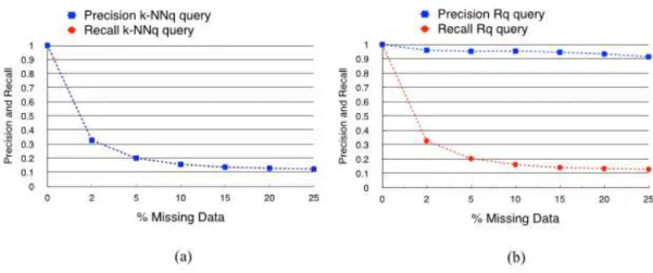
Figure 17 – Precision and recall forNDVIdatasets with MAR and MNAR assumptions . 82 Figure 18 – Precision and recall forWeathFordatasets with MAR assumption . . . 83
Figure 19 – Precision and recall forWeathFordatasets with MNAR assumption. . . 83
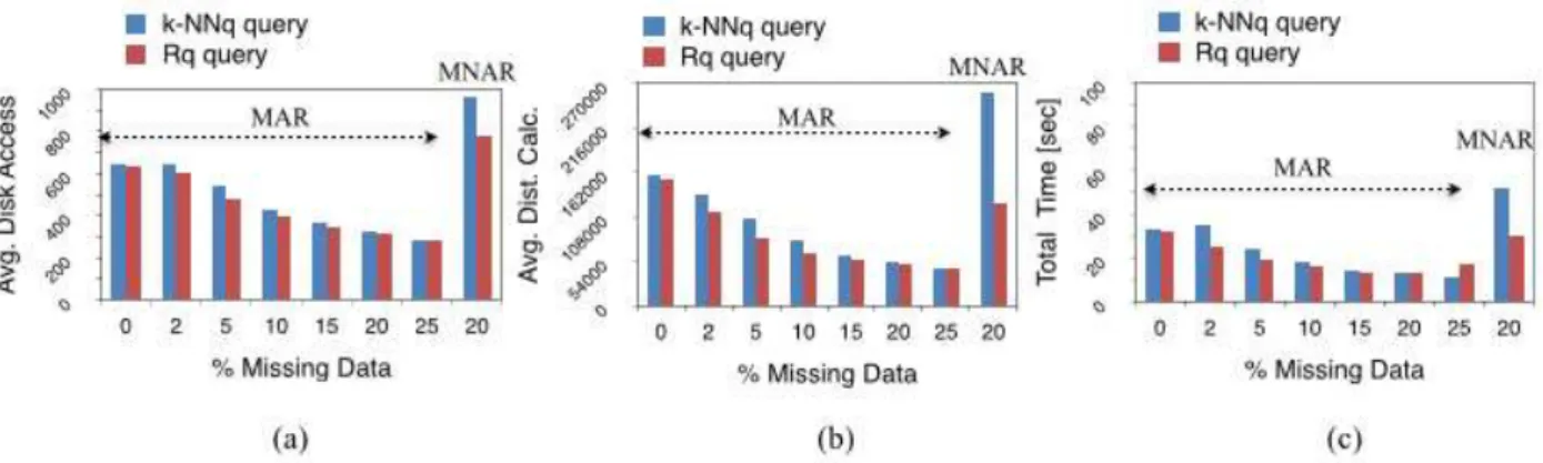
Figure 20 – Query performance forNDVIdatasets with MAR and MNAR assumptions . 84 Figure 21 – Query performance forWeathFordatasets with MAR assumption. . . 85
Figure 22 – Query performance forWeathFordatasets with MNAR assumption . . . 85
Figure 23 – Probability Density Function of the distances forWeathFor datasets with MAR assumption . . . 86
Figure 24 – Probability Density Function of the distances forWeathFor datasets with MNAR assumption . . . 87
Figure 25 – Example of data distribution in an internal node of an index structure with MAR and MNAR processes . . . 88
Figure 27 – Example of a node split using MSTSplitMiss algorithm . . . 98 Figure 28 – Example of a node split with duplicated representative . . . 98 Figure 29 – Example of equal feature vectors resulting from different images with missing
values . . . 99 Figure 30 – Example of a 10-Nearest Neighbour query withk-NNqandk-NNFMq . . . 100
Figure 31 – Desirable number of complete objects and objects withNullvalues to be
retrieved . . . 102 Figure 32 – Diagram of the experiments performed to evaluate the performance of the
Hollow-treemetric access method. . . 107
Figure 33 – Fractal dimension of the Sierpinski datasets with different amounts of missing data. . . 108 Figure 34 – Precision fork-NNqandk-NNFMqqueries processed overHollow-treeand
Slim-tree indexes forWeatherdataset . . . 110 Figure 35 – Recall for k-NNq and k-NNFMq queries processed over Hollow-tree and
Slim-tree indexes forWeatherdataset . . . 111 Figure 36 – Precision for 50-NNqand 50-NNFMq queries processed overHollow-tree
and Slim-tree indexes for synthetic datasets. . . 112 Figure 37 – Recall for 50-NNqand 50-NNFMqqueries processed overHollow-treeand
Slim-tree indexes for synthetic datasets. . . 112 Figure 38 – Precision for 100-NNqand 100-NNFMqqueries processed overHollow-tree
and Slim-tree indexes for synthetic datasets. . . 113 Figure 39 – Recall for 100-NNq and 100-NNFMq queries processed over Hollow-tree
and Slim-tree indexes for synthetic datasets. . . 113 Figure 40 – Precision for 200-NNqand 200-NNFMqqueries processed overHollow-tree
and Slim-tree indexes for synthetic datasets. . . 114 Figure 41 – Recall for 200-NNq and 200-NNFMq queries processed over Hollow-tree
and Slim-tree indexes for synthetic datasets. . . 114 Figure 42 – Precision for 500-NNqand 500-NNFMqqueries processed overHollow-tree
and Slim-tree indexes for synthetic datasets. . . 115 Figure 43 – Recall for 500-NNq and 500-NNFMq queries processed over Hollow-tree
and Slim-tree indexes for synthetic datasets. . . 115 Figure 44 – Precision and recall forRMqquery processed overHollow-treeand Slim-tree
indexes forWeatherdataset . . . 116 Figure 45 – Precision forRMqquery processed overHollow-treeand Slim-tree indexes
for synthetic datasets. . . 117 Figure 46 – Recall forRMqquery processed overHollow-treeand Slim-tree indexes for
Figure 48 – Efficiency parameters for 200-NNq and 200-NNFMqqueries for Weather
dataset . . . 119 Figure 49 – Average searching radius for 50-NNqand 50-NNFMqqueries for synthetic
datasets. . . 120 Figure 50 – Average searching radius 200-NNqand 200-NNFMq queries for synthetic
datasets. . . 120 Figure 51 – Total execution time for 50-NNqand 50-NNFMqqueries for synthetic datasets.121
Figure 52 – Total execution time for 200-NNq and 200-NNFMq queries for synthetic
datasets. . . 121 Figure 53 – Average number of disk accesses for 50-NNq and 50-NNFMq queries for
synthetic datasets. . . 122 Figure 54 – Average number of disk accesses for 200-NNqand 200-NNFMqqueries for
synthetic datasets. . . 122 Figure 55 – Average number of distance calculations for 50-NNqand 50-NNFMqqueries
for synthetic datasets. . . 123 Figure 56 – Average number of distance calculations for 200-NNq and 200-NNFMq
LIST OF ALGORITHMS
Algorithm 1 – randomSplit . . . 47
Algorithm 2 – minMaxSplit . . . 47
Algorithm 3 – MSTSplit . . . 48
Algorithm 4 – k-NNFq(sq,k) . . . 54
Algorithm 5 – randomSplitMiss . . . 95
Algorithm 6 – minMaxSplitMiss . . . 96
Algorithm 7 – MSTSplitMiss . . . 97
Algorithm 8 – RMq(sq,r) . . . 99
LIST OF TABLES
Table 1 – Illustration of the different mechanisms of missingness . . . 61
Table 2 – Bitmaps encoding with missing data . . . 67
Table 3 – Bitmaps index. . . 67
Table 4 – Database with missing values and VA-Files representation . . . 67
Table 5 – Summary of the techniques for missing data treatment at the index level . . . 68
Table 6 – Example of biased parameters of MNAR mechanism . . . 75
Table 7 – Distribution of missing data fork=5. . . 79
Table 8 – MAR datasets . . . 80
Table 9 – MNAR datasets . . . 80
Table 10 – Datasets used in the experiments and their characteristics. . . 106
LIST OF ABBREVIATIONS AND ACRONYMS
k-NNq . . . . k Nearest Neighbor query.
k-NNFq . . . k Nearest Neighbor query based on Fractal dimension.
k-NNFMq kNearest Neighbor query based on Fractal dimension for Missing data. BKT . . . Burkhard-Keller Tree.
BR-tree . . . Bit-string augmented R-tree. BST-tree . . Bisector tree.
CPU . . . Central Processing Unit DBM-tree Density-Balanced Metric tree. DBMS . . . Database Management System DWT . . . Discrete Wavelet Transform. FD . . . Fractal Dimension.
FQ-tree . . . Fixed Queries tree.
GHP-tree . Generalized Hyperplane tree.
GNAT . . . . Geometric Near-Neighbor Access Tree. Hollow-tree A variant of the Slim tree for missing data. I/O . . . Input / Output.
ICkNNI . . Incomplete Casek-Nearest Neighbors Imputation. IDWT . . . . Inverse Discrete Wavelet Transform.
INMET . . . Instituto Nacional de Meteorologia. kAndRange k nearest neighbor And Range query. kd-tree . . . k-dimensional tree.
KDD . . . Knowledge Discovery and Data Mining. kRingRange k nearest neighbor Ring Range query. M-tree . . . . Metric tree.
MAM . . . . Metric Access Method. MAR . . . Missing At Random. MBT . . . Monotonous Bisector Tree. MCAR . . . Missing Completely At Random. minDist . . Minimum Distance.
minMaxSplit Minimum Maximum Split.
minOccup Minimum Occupancy. MM-tree . . Memory-based Metric tree. MNAR . . . Missing Not At Random.
MOSAIC . Multiple One-dimensional Single-Attribute Indexes. MSTSplit . Minimal Spanning Tree Split.
MSTSplitMiss Minimal Spanning Tree Split for Missing data. MVP-tree . Multi-Vantage-Point tree.
NDVI . . . . Normalized Difference Vegetation Index. Rq . . . Range query.
randomSplit Random Split.
randomSplitMiss Random Split for Missing data. RMq . . . Range query for Missing data.
LIST OF SYMBOLS
m— Number of attributes.
sq— Query elementsq∈S.
r— Covering radius.
Rm— m-dimensional space. S— Data domain.
S— DatasetS⊂S.
d — Distance function.
s1,s2,s3— Elements of the data domainS. ∞— Infinite values.
=,̸=— Exact matching comparison operators.
<,≤, >,≥— Relational comparison operators.
x— Cartesian product operator.
Lp— Minkowski distance function family.
L2— Euclidean distance function. L1— Manhattan distance function. dE — Edit distance function.
s,t — String elements.
dQ— Quadratic distance.
dC— Canberra distance.
k— Number of nearest neighbors.
bp— Ball partitioning.
ghp— Generalized hyperplane partitioning.
rep,rep1,rep2— Representative elements. c— Minimum occupancy.
A,A1,A2— Tree nodes. D — Distance Exponent.
n— Cardinality of the dataset.
PC(r)— Number of pairs of objects within a distance r.
Kp— Proportionality constant.
R— Diameter of the dataset.
rf — Final radius.
log— Logarithm function.
e— Exponential function.
k′— Number of elements,k′<k.
r′f — Local final radius,r′f >rf.
k′′— Number of elements,k′′≤k.
L,L1,L2— Lists of elements.
I— Indicator variable of missingness.
X,Y — Random variables.
Xobs,Yobs— Observed values of the random variables X and Y, respectively.
Xmiss,Ymiss— Missing values of the random variables X and Y, respectively.
α — Parameter estimation.
ε— Gap of parameter estimation.
f — Probability Density Function.
kcom— Number of complete objects.
CONTENTS
1 INTRODUCTION . . . 27
1.1 Motivation . . . 27
1.2 Problem Definition and Main Objectives . . . 30
1.3 Summary of the Contributions . . . 33
1.4 Final Considerations. . . 34
2 SIMILARITY SEARCH IN METRIC SPACES . . . 37
2.1 Introduction . . . 37
2.2 Metric Spaces . . . 38
2.3 Distance Functions . . . 38
2.3.1 Examples . . . 38
2.3.2 Complexity Evaluation . . . 40
2.4 Similarity Queries . . . 40
2.5 Metric Access Methods . . . 42
2.6 Fractal Dimension for Similary Search . . . 48
2.6.1 Fractals and Fractal Dimension . . . 48
2.6.2 Fractal Dimension for k-NNq Queries . . . 51
2.7 Final Considerations. . . 55
3 MISSING DATA AND RELATED WORK . . . 57
3.1 Introduction . . . 57
3.2 Missing Data Theory . . . 58
3.2.1 Missing Data . . . 58
3.2.2 Legitimate or Illegitimate Missing Data . . . 59
3.2.3 Missing Data Mechanisms . . . 60
3.2.4 Ignorable and Non-ignorable Missingness . . . 61
3.2.5 Consequences of MCAR, MAR and MNAR . . . 62
3.3 Missing Data Treatment . . . 62
3.3.1 Treatment at the Data Level . . . 63
3.3.1.1 Case Deletion . . . 63
3.3.1.2 Missing Data Imputation . . . 63
3.3.1.3 Model-based Imputation . . . 64
3.3.2.1 Conventional Method . . . 65
3.3.2.2 BR-tree . . . 66
3.3.2.3 MOSAIC . . . 66
3.3.2.4 Extended Bitmaps . . . 66
3.3.2.5 Extended VA-Files . . . 66
3.4 Final Considerations. . . 68
4 THEORY OF MISSING DATA IN METRIC SPACES . . . 71
4.1 Introduction . . . 71
4.2 Formal Model for Missing Data in Metric Spaces . . . 74
4.2.1 Bias of Paremeter Estimation . . . 74
4.2.2 Formal Model for Missing Data . . . 75
4.3 Experimental Analysis . . . 77
4.3.1 Experimental Set-up . . . 78
4.3.1.1 Data Description . . . 78
4.3.1.2 Data Preparation . . . 78
4.3.1.3 Methodology . . . 79
4.3.2 Performance Results . . . 81
4.3.2.1 Effectiveness Parameters . . . 82
4.3.2.2 Efficiency Parameters . . . 84
4.3.2.3 Distance Concentration . . . 86
4.4 Final Considerations. . . 88
5 HOLLOW-TREE . . . 91
5.1 Introduction . . . 91
5.2 The Hollow-tree Access Method . . . 92
5.2.1 Indexing Technique . . . 92
5.2.1.1 SplitNode Policies . . . 94
5.2.1.2 ChooseSubtree Policies . . . 96
5.2.2 Similarity Queries . . . 97
5.2.2.1 The RMq Query . . . 98
5.2.2.2 The k-NNFMq Query . . . 98
5.3 Final Considerations. . . 102
6 HOLLOW-TREE EVALUATION . . . 105
6.1 Introduction . . . 105
6.2 Experimental Set-up . . . 105
6.3 Performance Metrics . . . 108
6.3.1 Effectiveness Parameters . . . 108
6.4 Experimental Results . . . 109
6.4.1 Effectiveness Assessment for k-NNq and k-NNFMq Queries . . . 109
6.4.2 Effectiveness Assessment for RMq Query . . . 116
6.4.3 Efficiency Assessment for k-NNq and k-NNFMq Queries . . . 118
6.5 Final Considerations. . . 124
7 CONCLUSION . . . 125
7.1 Main Contributions . . . 125
7.1.1 Background of Missing Data . . . 125
7.1.2 Formal Model for Missing Data in Metric Spaces . . . 126
7.1.3 Empirical Analysis for Missing Data in Metric Spaces . . . 126
7.1.4 Indexing Technique for Datasets with Missing Values . . . 127
7.1.5 Similarity Queries for Datasets with Missing Values. . . 127
7.1.6 Hollow-tree Access Method . . . 128
7.1.7 Extended Family of Metric Access Methods . . . 129
7.2 Future Work . . . 129
7.3 Publications Generated in this Ph.D. Work . . . 130
27
CHAPTER
1
INTRODUCTION
1.1
Motivation
Missing data is a common fact in real world applications. This may happen at the time of data collection or preprocessing due to errors in sampling, failures in transmission, in recording, storing, etc. For example, medical data often have missing diagnostic tests that would be relevant for estimating the likelihood of diagnoses or for predicting the effectiveness of a treatment. In spatial data, measurements can be missing because of sensor malfunction, low battery levels or insufficient resolution. Another example are census data where participants choose not to answer sensitive questions for personal or safety reasons. There are two forms of missingness: missing records, i.e., objects, and missing attribute values, i.e., some but not all attribute values from an existing object. While missing records may only be problematic in restricted situations (e.g., smaller size of the sample provides lower statistical power of the data), missing attribute values can influence the quality of data and the performance of the tasks that operate on such data.
28 Chapter 1. Introduction
One of the major aspects of missingness is the degree of randomness in which missing data occurred. Rubin (RUBIN,1976) developed a framework of inference about missing data and defined three classes of missingness, also known asmechanisms of missingness.Missing Completely At Random(MCAR) refers to the scenario where missingness of attribute values is independent of other attribute values (observed or missing). Missing At Random (MAR) corresponds to the scenario where missingness of attribute values depends only on observed values. Missing Not At Random (MNAR) corresponds to the scenario where missingness of attribute values depends on missing values. For example, consider a population ofnindividuals who had their blood pressure measured and a random sample of sizen′<nwho also had their weight measured. Missingness on weight measure is MCAR because it is randomly sampled and does not depend on any other value. Now, if we consider the same population that had their blood pressure measured and only those individuals with high blood pressure had their weight measured; missingness on weight measure is MAR because it depends on the observed values of blood pressure. Note that, if individuals with high blood pressure are likely to be overweight, it would appear that only overweight individuals had their weight measured and thus, missingness is MNAR, because missing values on weight depend on the measurements of weight where missing values occurred. As a consequence, the average value of the weight will be overestimated since low values are missing. Therefore, any parameter estimation of the weight measure will yield bias (i.e., underestimate or overestimate) in the results. The latter example shows how MNAR data can cause bias in the parameter estimation, therefore, determining the mechanism of missingness is very important, because it can influence the choice of an appropriate treatment for missing data.
The past few decades have witnessed a great development of techniques for missing data treatment. The main interest appeared first in the problems caused in surveys and census data (RUBIN,1976; SCHAFER,1997;LITTLE; RUBIN,2002;RUBIN,2004). Traditional approaches for dealing with missing data essentially includeCase DeletionandMissing Data Imputation. Case deletion consists of deleting the instances with missing values and performing the analysis using only complete instances. Despite being simple and amenable for implemen-tation, this method suffers from an important loss of relevant information. On the other hand, imputation methods aim at estimating missing values using relationships that can be identified in the observed values of the dataset. Several methods of imputation have been proposed in the literature, ranging from the most simpleMean or Mode Substitutionto the most sophisticated Multiple Imputation. However all these methods are either biased or computationally expensive. In addition, in many cases, some attributes have missing values because they are not relevant for certain objects, therefore, any imputation method would become inappropriate.
non-1.1. Motivation 29
dimensional and high-dimensional data are usually stored and retrieved following a similarity criteria, and the process is calledSimilarity Search. Similarity search involves finding objects that are similar to a given query object based on a similarity measure. The searching process is usually performed with range query or nearest neighbor query, often using an index structure to speed up the searching process. There are two families of access methods that provide indexing support for similarity search:Multidimensional Access MethodsandMetric Access Methods(MAMs). Multidimensional access methods, such as R-tree (GUTTMAN,1984) and kd-tree (BENTLEY, 1975;BENTLEY,1979), are created to support efficient selection of objects based on spacial properties. Many multidimensional access methods have been proposed in the literature (SAMET, 1984;GAEDE; GüNTHER,1998) aiming at improving the performance of the similarity queries over multimedia datasets. However, they are not appropriate for datasets where the only available information is the distances between objects, like DNA datasets. This fact is one of the reasons that led to the development of metric access methods.
Metric access methods are fundamental to organize and access both non-dimensional and high-dimensional data. They employ index structures to organize the data based on a distance function and the space is divided into regions using a set of chosen objects, calledrepresentatives, and their distances to the rest of the objects in the space. A metric space is a pair(S,d), whereS
denotes a data domain andd:S×S→R+ is a distance function that satisfies the symmetry, the
non-negativity and the triangle inequality properties. A datasetSis in a metric space whenS⊂S.
When a query is issued, the properties of the metric space are used to prune the searching space in order to speed up the query process. Many metric access methods have been proposed in the literature (HJALTASON; SAMET,2003;SAMET,2006), however, they were all designed to perform only on complete datasets; and when applied on datasets with missing values, they lose their functionalities and suffer from poor query performance.
Missing attribute values are a major concern to perform similarity search over data indexed in a metric space. Similarity search involves comparison operations based on a distance function that helps comparing pairs of objects in a data domainSand returns a numerical value
30 Chapter 1. Introduction
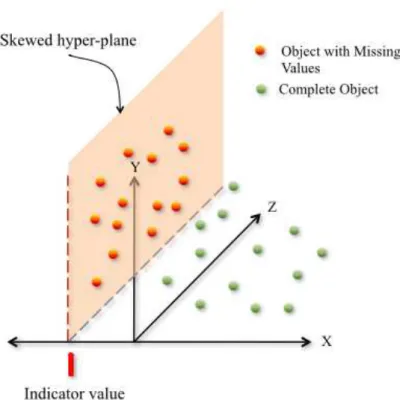
Figure 1 – Example of objects with missing values projected in a three-dimensional space using an indicator value.
1.2
Problem Definition and Main Objectives
Advanced database applications often deal with incomplete data. Such applications usually involve large datasets of non-dimensional or high-dimensional data objects. Therefore, there is always a possibility of having erroneous or missing data.
The most popular approach used to make the existing indexing techniques operational on incomplete datasets is to use an indicator variable to identify the missing values, then employ a traditional indexing technique to index the dataset. For example, if the domain of an attribute are the positive integers, then, a value of -1 can be used to denote the missing values. Data stored in relational Database Management Systems (DBMS) employ the attribute state ofNullvalues to indicate missing data. With this scheme and for a multidimensional indexing technique, all the objects with missing values on a given dimension will be projected into the same value of the hyper-region (see Figure1), causing skew in the indexed space. When the proportion of missing values is large, it will result in a highly skewed data space.
1.2. Problem Definition and Main Objectives 31
Figure 2 – Example illustrating objectssiandsjassinged to a tree nodeA, wheresi∈Abecaused(si,Rep)<r, and
sj∈/Abecaused(si,Rep)>r.
useful for multidimensional indexing techniques and they are impractical for metric indexing techniques.
On the other hand, most of the distance functions are designed to measure the similarity between complete objects, and it is not feasible to apply them on data with unknown (i.e., missing) values. For instance, if we consider the objects s1,s2∈Swith attribute values denoted bys1,i,s2,ifor 1<i<m, wheremis the number of attributes. The squared Euclidean distance betweens1ands2
is the sum of the squared differences between the mutual attribute values, i.e.,∑mi=1(s1,i−s2,i)2.
If one of the objects has missing values on some attributes, the differences between the mutual attributes with missing values are unknown, and consequently the distance measure becomes undefined.
32 Chapter 1. Introduction
Figure 3 – Data distribution in nodes where (a) representative is complete, (b) representative has missing values.
random, distance measures are prone to skew. In particular, objects with missing values tend to shrink the subspaces where missingness occurred, causingDistance Concentration. The major problem here is that if the representatives are chosen among the objects that have missing values, the bounding regions of the associated nodes are likely to shrink because of smaller distances (see Figure3). Moreover, for the same reason, representatives with missing values potentially hold more objects during the indexing and searching processes, independently from if they are similar or not. This fact can lead to inconsistency in the index structure. Therefore, when similarity queries are issued, it is more likely to have irrelevant objects in the query response (false positives), having relevant ones not included in the response (false negatives), which leads to poor query performance.
The performance of a metric access method regards its overall execution time, which in turn depends mainly on the number of distance calculations and the number of disk accesses it needs to execute the similarity queries. However, when dealing with data that have missing attribute values, the retrieval accuracy (i.e., effectiveness of the similarity queries) becomes another major measurement of the index quality. The reason is that missing attribute values may introduce changes to the distribution of data in the metric space and, subsequently, cause inconsistency in the data structure, leading to inaccurate query response. In the course of this Doctoral work, we seek to demonstrate that problem, thus, we established three major hypotheses to guide our work:
1. Data with the MAR mechanism cause distortion in the internal structure of the metric index and affect significantly the effectiveness parameters of the query process.
1.3. Summary of the Contributions 33
3. The performance of a metric access method in incomplete high-dimensional spaces are influenced differently when data are MAR and when data are MNAR.
To demonstrate the validity of these hypotheses, this research was conducted with the following specific goals:
1. Investigate the key issues involved when indexing and searching datasets with missing attribute values in metric spaces.
2. Identify the effects of each mechanism of missingness on the metric access methods when applied on incomplete datasets.
3. Based on these effects, formalize the problem of missing data in metric spaces, proposing a ”Model of Missingness”.
4. Based on the formal model of missingness, develop new techniques to support similarity search over large and complex datasets with missing values, in order to overcome the limitations of metric access methods and allow traditional methods to explore the available data while preserving their functionalities and their characteristics.
1.3
Summary of the Contributions
In this Ph.D. work, we identified the issues related to missing data when indexed and searched in metric spaces, and we used them to establish a formal Model of Missingness able to describe missingness in metric spaces. The analyzes of the metric access methods when applied on incomplete datasets (see the upcoming chapter 4) led us to identify two main issues. The first issue is related to distortions that occur in the internal structure of the index when the mechanism of missingness is random. The second issue concerns the skew of the index structure caused by the MNAR mechanism. The findings suggest that the effects of the MAR and the MNAR mechanisms described in the statistics literature apply also to the metric spaces when incomplete datasets are indexed. With regard to the MAR mechanism, objects with missing values may change the distribution of data in the space while keeping the overall sparseness (i.e., volume) of the metric space. With regard to the MNAR mechanism, objects with missing values are capable to skew the distribution of data in the space causing a significant distance concentration.
34 Chapter 1. Introduction
with missing values. Both return two separated lists: one for the complete objects retrieved and another for objects with missing values. The new query types are:
∙ The range query for missing data –RMq(sq,r): It receives a query centersqand a query radius r as parameters, and returns the complete objects and the objects with missing values that are distant at most at the covering radiusrfromsq.
∙ ThekNearest Neighbor query based on Fractal Dimension for Missing data –k-NNFMq(sq,k): It employs the fractal dimension of the dataset and the local density of the query region to search for similar objects and filter data in the query response. The query response is composed of two lists: A list of complete objects and a list of objects with missing values.
We applied these techniques to the Slim-tree access method (TRAINA et al., 2002), which led to the development of a new variant, called Hollow-tree, to support datasets with missing values.
Existing metric access methods do not support indexing data with missing attribute values. The proposedHollow-treecan efficiently index and search data with missing attribute values. Prior approaches for missing data treatment provided support for multidimensional access methods, which resulted in a severe performance that is often worse than the sequential scan when the number of missing values is significantly high (OOI; GOH; TAN,1998). Other approaches supported indexing and searching incomplete datasets in non-hierarchical indexing techniques (CANAHUATE; GIBAS; FERHATOSMANOGLU,2006). These techniques exhibit a linear performance with respect to dimensionality and amount of missing data, however, they are not suitable to process large and complex datasets. The ability to accommodate non-dimensional and high-dimensional datasets with missing data makes theHollow-treemore appropriate for nowadays applications.
1.4
Final Considerations
This chapter presented an overview of this Doctoral dissertation with a description of the facts that motivated this project, the definition of the problem, the main objectives and contributions of this work. The remaining chapters of the thesis are as follows:
∙ Chapter 2 gives an introduction to the basic concepts of the similarity search in metric spaces, including an overview of the Fractal Theory concepts used to boost similarity queries in metric spaces. This chapter gives a background for the rest of the thesis.
1.4. Final Considerations 35
∙ Chapter 4 studies the effect of missing data when indexed in metric spaces. A formal model for missing data is defined to provide an understanding of the effects of distortion and skew caused by missingness in metric spaces.
∙ Chapter 5 describes the proposed techniques for indexing and querying incomplete datasets.
∙ Chapter 6 is dedicated to the performance evaluation of the proposed techniques.
37
CHAPTER
2
SIMILARITY SEARCH IN METRIC SPACES
2.1
Introduction
In classical databases systems, where most of the attributes are either textual or numerical, the fundamental search operation is matching, i.e., given a query object, the system finds the objects in the database whose attributes match those specified in the query object. The result of this type of queries is, typically, a set of objects that are, in some sense, the same as the query object. In multimedia databases, this kind of operation is not appropriate. In fact, due to the complexity of multimedia objects, such as images, audio and video collections, DNA or protein sequences, among others; matching is not sufficiently expressive. Instead, objects should be searched by similarity criteria. Similarity search involves a collection of objects (e.g., documents, images, videos) that are characterized by a set of relevant features and represented as points in the high-dimensional space. Given a query in the form of a point in the space, similarity queries search for the nearest (most similar) object to the query object. The particular case of the Euclidean space is of a major importance for a variety of applications, like databases and data mining, information retrieval, data compression, machine learning and pattern recognition, etc. Typically, the features of the objects are represented as points in theRmand a distance function
is used to measure the degree of similarity between them.
38 Chapter 2. Similarity Search in Metric Spaces
2.2
Metric Spaces
A metric space is defined as a pair(S,d), whereS denotes a domain (universe) of valid objects
(elements, points) andd :S×S→R+ a distance function. The distance function is called a
metric if it satisfies the following properties: Given any objectss1,s2,s3∈S:
∀s1,s2∈S, d(s1,s2) =d(s2,s1) symmetry,
∀s1,s2∈S, 0<d(s1,s2)<∞ non-negativity,
∀s1∈S, d(s1,s1) =0 identity,
∀s1,s2∈S, d(s1,s2) +d(s2,s3)≥d(s1,s3) triangle inequality.
The distance function d measures the distance between two objects and returns a real non-negative value, which assesses the similarity degree between them. The smaller the distance measure is, the closer or more similar the objects are; the larger the distance measure is, the less similar the objects are.
2.3
Distance Functions
Distance functions are often associated to a specific application or a specific data type. Depending on the returned value, typically, there are two groups of distances:
∙ Discret - the distance function returns a small set of discrete values, such as the Edit distance,
∙ Continuous- the distance function returns a set of values whose cardinality is very large or infinite, such as the Euclidean distance.
2.3.1
Examples
Some of the most popular distance functions include the Minkowski distances, Edit distance and the Quadratic Form distance.
Minkowski Distance
Minkowski distances represent the family of metric distances, calledLpmetrics. They are defined onm-dimensional vectors of real numbersX andY as follows:
Lp(X,Y) = p s
m
∑
i=1
|xi−yi|p p≥1 (2.1)
Special cases of such metrics are the Euclidean (L2) and the Manhattan, or city bloc, (L1)
2.3. Distance Functions 39
are very appropriate to measure the distance between gray-level or color histograms and between vectors of features extracted from images.
Levenshtein Distance
The Levenshtein (LEVENSHTEIN,1965), or edit, distancedE(s,t)for strings counts the mini-mum number of edit operations (insertions, deletions, substitutions) needed to transform a string sinto a stringt.
Quadratic Form Distance
The Euclidean distanceL2, used to measure the distance between color histograms, does not
identify the correlations between the components of the histograms. A distance function that has been successfully applied to image databases (FALOUTSOSet al.,1994) and that has the power to model dependencies between different components of the histogram is provided by the class of quadratic form distance functions (HAFNERet al.,1995;SEIDL; KRIEGEL,1997). Therefore, the distance measure of twom-dimensional vectors is based on anmxmmatrixA= [ai j], where the weightsai j denote the similarity between the componentsiand jof the vectors
→
x and →y, respectively:
dQ(→x,→y) = q
(→x −→y)T·A·(→x −→y) (2.2)
When the matrixAis equal to the identity matrix, then we have the Euclidean distance. The quadratic form distance function is computationally expensive as the image color histograms are typically high-dimensional vectors, consisting of 64 or 256 distinct colors.
Canberra Distance
Similar to the Manhattan distance, Canberra distance is however more restrictive, since the absolute difference of the feature values is divided by the sum of their absolute values. It is formally defined form-dimensional vectorsX andY as follows:
dC(X,Y) = m
∑
i=1
|x[i]−y[i]|
|x[i]|+|y[i]| (2.3)
This distance is very sensitive to small changes, and it has been used in different areas such as DNA sequences in bioinformatics, and also in computer intrusion detection.
40 Chapter 2. Similarity Search in Metric Spaces
2.3.2
Complexity Evaluation
The time required to compute the Lpand the Canberra distances is linear with respect to the number of components in the feature vectors. The Levenshtein distance employs a dynamic algorithm, thus, it is executed with quadratic complexity on the number of letters in both strings. The Quadratic form distance is even more expensive because it requires multiplications by a matrix. Thus, it is evaluated inO(n3). Other distance functions that measure the distance between
sets of objects can be up toO(n4). Therefore, distance functions are generally considered as time
consuming operations, and most of the indexing techniques for similarity search try to reduce the number of distance evaluations to speed up the searching process.
2.4
Similarity Queries
Similarity queries are defined by a query object and some selectivity criterion. The answer to the query is the set of objects that are close to the query object and satisfy the selectivity criterion. There are two types of similarity queries:
Range Query
This is the most common type of query that is used in almost every application. Provided an objectsqand a covering radiusr, theRq(sq,r)query retrieves all the objects which are within the covering radiusrfromsq(see Figure4a). Formally:
Definition 1. Given a query centersq∈Sand a query distancer, aRange queryRq(sq,r)in a metric space(S,d)retrieves all the objectssi∈Ssuch thatd(sq,si)<r.
Example: ”Find all the restaurants that are within a distance of two miles from here”.
k-NNq Query
Provided an objectsqand an integerk, thek-NNq(sq,k)query retrieves theknearest neighbors to the objectssq(see Figure4b). Formally:
Definition 2. Given a query center sq∈Sand an integerk>0, a k-Nearest Neighbor query k-NNq(sq,k)in a metric space(S,d)retrieves thekobjects closest tosq, based on the distance
functiond.
Example: ”Find the five closest restaurants to this place”.
2.4. Similarity Queries 41
Figure 4 – (a) Range queryRq(sq,r), and (b)k-nearest neighbor queryk-NNq(sq,k), with k = 5.
dataset is very large (e.g., in the order of hundreds of thousands or millions of objects) and the distance function is computationally expensive, the sequential scan of the entire dataset is not an adequate option. One good alternative is to structure the objects of the dataset in a way that allows to find the required objects efficiently without looking at every object of the dataset. In traditional database management systems, where sorting (or ordering) is the basis for efficient searching, index structures, such as B-tree (BAYER; MCCREIGHT,1973), are used to search through the objects of the dataset. Although, sorting numbers, text strings or dates is easier, it is not obvious to order complex data, like images. Thus, the traditional index structures cannot be used to search complex data in general.
Multimedia applications require that access methods satisfy the following properties:
∙ Efficiency:Unlike traditional access methods which only aim at minimizing the number of disk accesses, index structures for similarity search need also to consider the CPU costs given by the number of distance calculations, since the distance functions are generally considered as time consuming operations.
∙ Scalability:Due to the size of modern multimedia data repositories which are usually in the order of millions of objects, the access methods should also perform well when the size of the database grows.
∙ Dynamicity:Access methods need to support insertions and deletions of objects from the index structures.
∙ Data type independency: Access methods need to perform well on all possible data types.
42 Chapter 2. Similarity Search in Metric Spaces
There are two families of access methods that support similarity search on multimedia datasets;Mulidimensional Access Methods, also well-known as spacial access method (SAMs), andMetric Access Methods(MAMs). Multidimensional access methods are created to support efficient selection of objects based on spacial properties. These methods use the idea of parti-tioning the indexed space into subsets, called equivalent classes, and group into sets objects that have some property in common, e.g., the first coordinate of a vector is lower than three. For example, kd-trees (BENTLEY,1975;BENTLEY,1979) or quad-trees (SAMET,1984) use a threshold (value of a coordinate) to divide the given space into subsets. On the other hand, R-tree (GUTTMAN,1984) groups objects in an hierarchical organization using the minimum bounding rectangle. Many spacial access methods have been proposed in the literature (see (SAMET,1984; GAEDE; GüNTHER,1998;SAMET,2006) for a comprehensive survey), aiming at improving the performance of the similarity queries over multimedia datasets. However, they do not satisfy the properties described above. In fact, spacial access methods can only index multidimensional vector spaces; thus, they are not appropriate for datasets where the only available information is the distances between objects, like DNA datasets. Moreover, with regard to query performance, only I/O cost given by the number of disk accesses is considered, while CPU cost of the distance calculations is ignored. In the case of high-dimensional vector spaces, the computation of the distances should not be ignored, instead, an additional optimization is needed in order to mini-mize the number of computed distances. These considerations led to the development of metric access methods (UHLMANN,1991).
2.5
Metric Access Methods
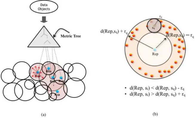
Metric access methods (MAMs) employ an index structure to organize the objects of a given dataset in an hierarchical tree structure, calledMetric Tree; based on a distance function that satisfies the metric properties; symmetry, non-negativity and triangle inequality. Metric trees aim at dividing the space into regions, where objects that are close to each other are grouped together (see Figure5a). Ideally, each region in the space is associated to a node in the tree, where leaf nodes store the data objects, the internal nodes store the pointers to the lower levels of the tree, and the root node holds the entire data space. Similarity search in metric trees involves accessing only the nodes where the relevant objects can be found and disposing of the nodes that do not contain relevant objects. This is often achieved by applying the triangle inequality property of the distance function, in order to speed up the searching process and reduce the number of disk accesses and the number of distance calculations (see Figure5b). The performance of similarity queries depend mainly on the pruning ability of the underlying access method, which in turn depends on the space partitioning technique.
2.5. Metric Access Methods 43
Figure 5 – An example of a metric space and a range query: (a) A metric index structure, (b) a range query.
to their distances to the representatives. Burkhard and Keller (BURKHARD; KELLER,1973) defined two basic partitioning techniques:
1. theballpartitioningbp, and
2. thegeneralized hyperplanepartitioningghp.
In the ball partitioning, one representativerepis chosen and a radiusris defined to split the objectssi, 1<i<n, into two groups as follows:
bp(si,rep,r) =
0 i f d(si,rep)≤r,
1 i f d(si,rep)>r.
In the hyperplane partitioning, two representativesrep1,rep2are chosen and the objects
si, 1<i<n, are split into two groups according to their distances to the representatives as follows:
ghp(si,rep1,rep2) =
0 i f d(si,rep1)≤d(si,rep2),
1 i f d(si,rep1)>d(si,rep2).
44 Chapter 2. Similarity Search in Metric Spaces
Vantage-Point tree (VP-tree) of Yianilos (YIANILOS,1993) are based on the ball partitioning technique, as they partition the objects into two groups according to a representative, called "vantage point". In order to reduce the number of distance calculations between the query object and the representatives, Baeza-Yates (BAEZA-YATESet al.,1994) proposed an extension of the VP-tree, called the Fixed Queries tree (FQ-tree), which uses the same vantage point in all the nodes that belong to the same level. However, this method suffers space complexity that grows super-linearly because the objects selected as representatives are duplicated. Another extension of the VP-tree is the Multi-Vantage-Point tree (MVP-tree) (BOZKAYA; ÖZSOYOGLU,1997; BOZKAYA; ÖZSOYOGLU,1999). While VP-trees use different representatives at the lower level of an internal node, MVPT-trees employ only one, that is, all children at the lower level use the same representative. This allows to have less representatives while the number of partitions is preserved.
The Bisector tree (BST-tree)(KALANTARI; MCDONALD,1983) is the first access method that uses the generalized hyperplane partitioning technique. BST-tree is a binary tree that is built recursively, choosing two representatives at each node and applying hyperplane partitioning. For each node, the covering radius is established as the maximum distance between the representative and the objects in its subtree and it is stored in the node. The first improvement of the BST-tree is the Voronoi Tree (VT) (DEHNE; NOLTEMEIER,1987). VT-trees use two or three representatives in each internal node and have the property that the covering radii are reduced when moving to the bottom of the tree. This provides better packing of objects in the subtrees. Another variant of BST-tree, called Monotonous Bisector Tree (MBT), is proposed by Noltemeier et al. (NOLTEMEIER; VERBARG; ZIRKELBACH,1992a; NOLTEMEIER; VERBARG; ZIRKELBACH,1992b). The idea of this structure is that the representative of each internal node, except the root node, is inherited from its parent node. This technique allows to use less representatives and, consequently, reduces the number of distance calculations during the searching process. The Generalized Hyperplane tree (GHP-tree) proposed by Uhlmann (UHLMANN,1991) is nearly the same as the BST-tree. It consists of partitioning the dataset recursively using the generalized hyperplane technique. The main difference is that, during a searching process, the covering radii are not used as pruning criterion, instead, the hyperplane between the representatives of two nodes is used to choose which subtree should be visited. The Geometric Near-Neighbor Access Tree (GNAT) of Bin (BRIN,1995) is considered as a refinement of the Ball Decomposition tree. In addition to the representatives and the maximum distance, the distance between pairs of representatives are also stored, in order to be used by the triangle inequality for further pruning in the searching space.
2.5. Metric Access Methods 45
each entry includes a pointer to the subtree and its covering radiusr. Each node contains at least cand at mostCentries, wherec≤C/2. The Slim-tree (TRAINAet al.,2002) is an extension of the M-tree that includes a technique, called "Slim-Down", which aims at reducing the amount of overlap between the nodes. Other dynamic MAMs include the Omni-family (FILHOet al., 2001), the Density-balanced Metric tree (DBM-tree) (VIEIRAet al.,2010), the Memory-based Metric tree (MM-tree) (VENTURINI; TRAINA; TRAINA,2007) and the Onion-tree (CARéLO et al.,2011).
Slim-tree
The Slim-tree (TRAINAet al.,2002) is a dynamic and balanced metric tree that aims to speed up insertion and node splitting while reducing overlap between the nodes. The metric tree is built from the bottom to the root and objects are grouped into fixed size disk pages, each page corresponding to a node. A Slim-tree is organized in a hierarchical structure, where a node holds a representative object, a covering radius and a subset of objects that are inside the covering radius. Since the size of a page is fixed, the nodes hold a limited number of objectsC. Slim-trees support two types of nodes, leaf nodes and index (internal) nodes (see Figure6). The leaf nodes hold all the objects stored in the index and the structure is:
lea f_node[array o f <Oidi,d(si,srep),si>],
whereOidiis the identifier of the objectsiandd(si,srep)is the distance between the objectsiand the representative of the leaf nodesrep. The index nodes hold the representatives of the nodes in the lower level and pointers that point to these nodes. The structure is:
index_node[array o f <si,ri,d(si,srep),Ptr(si),NEntries(Ptr(si))>],
wheresiis the representative of the subtree pointed byPtr(si)andriis the covering radius of its region. The distance between the entrysi and the representativesrepof this node is kept in d(si,srep). The pointerPtr(si)points to the root node of the subtree rooted bysi, for which the number of entries is kept inNEntries(Ptr(si)).
46 Chapter 2. Similarity Search in Metric Spaces
Figure 6 – Slim-tree index structure.
object is inserted in a leaf node. When a node overflows,SplitNodeprocedure is executed to split the node into two nodes. Subsequently, a new node is allocated at the same level and the objects are distributed among the nodes. Slim-tree provides three policies forChooseSubtreeprocedure:
1. random- Chooses randomly one of the qualifying nodes.
2. minDist- Chooses the node for which the representative has the shortest distance to the new object.
3. minOccup - Chooses the node that has less objects (minimum occupancy) among the qualifying nodes. This is the default method used by Slim-tree, as it has, in general, the best performance.
TheminOccup policy requires the number of objects in the qualified nodes. This is provided by theNEntriescomponent stored in the parent node that points to these nodes. The splitting policies of the Slim-tree are illustrated in the Algorithms 1, 2 and 3.
1. randomSplit- The representatives are chosen randomly among the objects in the node and the remaining objects are assigned to the node having the closest representative (see the details in Algorithm 1).
2.5. Metric Access Methods 47
Algorithm 1:randomSplit Data: NodeAto be split
Result: NodesA1andA2with their representativesrep1andrep2, respectively
1 Choose randomlyrep1fromA; 2 Choose randomlyrep2fromA; 3 whilerep2=rep1do
4 Choose randomlyrep2; 5 end
6 Set the new representatives,rep1for nodeA1andrep2for nodeA2; 7 foreach object siof the node Ado
8 ifd(si,rep1)<d(si,rep2)then 9 Addsito nodeA1;
10 else
11 Addsito nodeA2; 12 end
13 end
14 end
15 Return(A1,rep1),(A2,rep2);
Algorithm 2:minMaxSplit Data: NodeAto be split
Result: NodesA1andA2with their representativesrep1andrep2, respectively
1 foreach object siof the node Ado
2 foreach object sj̸=siof the node Ado 3 Setsiforrep1and setsjforrep2;
4 Create temporary nodesA′1andA′2withrep1andrep2, respectively; 5 Distribute the objects of the nodeAbetweenA′1andA′2;
6 Save the covering radii of the resulting nodes;
7 end
8 end
9 Select the pair(rep1,rep2)that minimizes the covering radii of the resulting nodes; 10 Set the new representativesrep1for nodeA1andrep2for nodeA2;
11 foreach object siof the node Ado 12 ifd(si,rep1)< d(si,rep2)then 13 Addsito nodeA1;
14 else
15 Addsito nodeA2; 16 end
17 end
18 end
19 Return(A1,rep1),(A2,rep2);
48 Chapter 2. Similarity Search in Metric Spaces
performance.
Algorithm 3:MSTSplit Data: NodeAto be split
Result: NodesA1andA2with their representative objectsrep1andrep2, respectively
1 Create a temporary nodeA′;
2 foreach object siof the node Ado 3 Add objectsitoA′
4 end
5 Perform the MST algorithm onA′;
6 Set the new representativesrep1for nodeA1andrep2for nodeA2; 7 foreach object siof the node Ado
8 ifd(si,rep1)< d(si,rep2)then 9 Addsito nodeA1;
10 else
11 Addsito nodeA2; 12 end
13 end
14 end
15 Return(A1,rep1),(A2,rep2);
minOccuppolicy for ChooseSubtree procedure allows to generate nodes with higher occupancy rates, leading to a smaller number of disk accesses. MST policy for SplitNode procedure is the fastest splitting algorithm among the available policies when the capacity of the nodesCis greater than 20 (TRAINAet al.,2002). Slim-Down algorithm allows producing thinner trees, reducing the number of distance calculations during the searching process. Therefore, when combined, these algorithms allow to Slim-tree to achieve a performance significantly better than the M-tree.
2.6
Fractal Dimension for Similary Search
In this section, we present concepts involving the use of the Fractal theory to allow improving algorithms that perform similarity search.
2.6.1
Fractals and Fractal Dimension
Fractal geometry provides a mathematical model for many complex objects found in the nature (MANDELBROT,1983;PENTLAND,1984), such as coastlines, mountains, and clouds. These objects are too complex to possess characteristic sizes and to be described by traditional Euclidean geometry. Self-similarity is an essential property of fractals in the nature and can be quantified by their ”Fractal Dimension” (FD).
2.6. Fractal Dimension for Similary Search 49
Figure 7 – Sierpinski triangle: first few steps of its recursive construction.
triangle”. Each small triangle is a miniature replica of the whole triangle. In general, the essence of fractals is this self-similarity property: parts of the fractal are similar to the whole fractal.
There is an infinite family of fractal dimensions, each one making sens in a different situation. Among them, we find the Hausdorff Fractal Dimension, the Information Fractal Dimensionand theCorrelation Fractal Dimension. For similarity search, the employed fractal dimension FD is commonly associated to the correlation fractal dimensionD. Correlation fractal
dimension measures the probability that two randomly chosen objects are within a certain distance from each other. Different methods have been proposed to estimateD, such as
pair-counting and box-pair-counting. The pair-pair-counting approach involves calculating the number of pairs of elements within a given distance from each other. The average number of neighborsCr within a given radiusris exactly twice the total number of pairs within the distancer, divided by the number of elementsNin the dataset. The box-counting approach (SCHROEDER,1991) consists of imposing a nested hypercube grids on the data, followed by counting the occupancy of each grid cell, thus focusing on individual elements instead of pairs of elements. The sum of the squared occupanciesS2(r)for a particular grid side lengthris defined asS2(r) =∑iCi2, whereCiis the count of elements in theith cell. The box-counting approach can be employed to measureD of any dataset and has been employed in various application fields. The reason for its
dominance lies in its simplicity and automatic computability.
The FD has been used as a powerful support for texture analysis and segmentation (CHAUDHURI; SARKAR,1995;IDA,1998), shape measurement and classification (NEIL; CURTIS,1997;BRUNOet al.,2008), attribute selection and dimensionality reduction (BERCH-TOLD; BöHM; KRIEGAL,1998;PAGEL; KORN; FALOUTSOS,2000;TRAINAet al.,2010), analysis of spatial access methods (FALOUTSOS; KAMEL,1994; KAMEL; FALOUTSOS, 1994;BELUSSI; FALOUTSOS,1995), analysis of metric trees (TRAINA; TRAINA; FALOUT-SOS,2000), indexing (BöHM; KRIEGEL,2000), join selectivity estimation (FALOUTSOSet al.,2000) and selectivity estimation for nearest neighbor queries (BERCHTOLDet al.,1997; PAPADOPOULOS; MANOLOPOULOS,1997;VIEIRAet al.,2007).
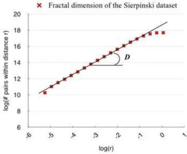
Many real datasets are fractals (SCHROEDER,1991;TRAINA; TRAINA; FALOUTSOS, 2000), i.e., their parts are self-similar. Self-similar datasets, by definition, obey a power law as follows (FALOUTSOS; KAMEL,1994):
50 Chapter 2. Similarity Search in Metric Spaces
Figure 8 – Distance plot of the Sierpinski dataset and its fractal dimension.
numberkof neighbors within a given distanceris proportional torraised toD, whereD is the
correlation fractal dimension of the dataset:
PC(r) =Kp×rD (2.4)
whereKpis a proportionality constant.
The graph of the number of pairs of objects within a distancerversus the distance r is called “Distance Plot”. For any dataset associated with a metric that estimates the pairwise distances between its objects, the graph of the distance plot can be drawn, even if the dataset is not in a dimensional domain. Plotting this graph in log-log scale, for the majority of real datasets, results in an almost straight line for a significant range of distances. The slop of the line that best fits the resulting curve in the distance plot is the "Distance ExponentD". Note that, measured
in this way,D closely approximates the theoretical correlation fractal dimension of the dataset.
Figure8shows the distance plot of the Sierpinski dataset and the resulting fractal dimensionD
obtained measuring the slop of the line.
The following observation states a useful property of the distance exponent.
Observation 1. The distance exponent is invariant to sampling, i.e., the power law holds for subsets of the dataset (FALOUTSOSet al.,2000).
2.6. Fractal Dimension for Similary Search 51
Figure 9 – An example of the similarity queries performed over a metric index: (a) range query, (b)k-NNqquery.
PC(r)multiplied by the sampling rate p, on the average. Therefore, the slop of the line in the plot will not change; it will only lower the position of the plot by log(p).
2.6.2
Fractal Dimension for
k
-
NN
qQueries
52 Chapter 2. Similarity Search in Metric Spaces
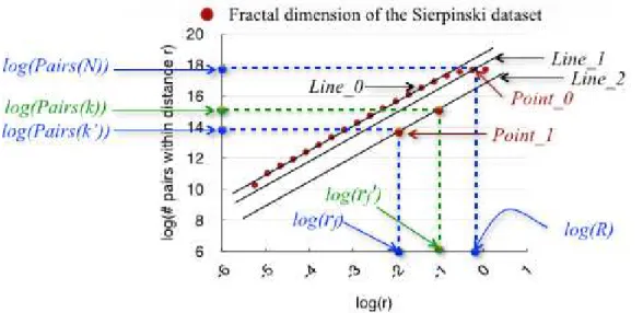
Figure 10 – How to use the Distance Plot to obtain the final radiusrf.
the subtrees to be visited. However, managing the priority queues and the dynamic radius can be very expensive and, consequently, can reduce the performance of the algorithm.
In order to speed upk-NNqqueries, Vieira et al. (VIEIRAet al.,2007) proposed a new variant, calledk-NNFq(sq,k), that estimates a final radiusrf for thek-NNqqueries, allowing to prune most of the objects that are not likely to be relevant.k-NNFq(sq,k)query performs in three steps:
1. Estimate a limiting radius for thek-NNqquery,
2. Perform a composed Range andk-NNqqueries,
3. If the required numberkof objects were not obtained, refine the searching procedure.
In the first step ofk-NNFqalgorithm, the final radiusrf is estimated using the distance plotD of the dataset and a pointPoint_0=Dlog(R),log(Pairs(N))E. Figure10illustrates how
to use the distance plot to estimate the final radiusrf. It is obtained by converting the numberk of objects into the corresponding covering radius as follows:
rf =R×e(log(k−1)−log(N−1))/D (2.5)
whereRis the diameter of the dataset,Nis the total number of objects in the dataset andD is
the fractal dimension of the dataset. The diameterRcan be obtained from the index structure as the covering radius of the root node in the tree.