50 years return period wet-snow load estimation based on weather station data for overhead line design purpose

(1)

NHESSD

2, 5139–5170, 2014

50 years return period wet-snow load

estimation

H. Ducloux and B. E. Nygaard

Title Page

Abstract Introduction

Conclusions References

Tables Figures

◭ ◮

Back Close

Full Screen / Esc

Printer-friendly Version

Interactive Discussion

P

a

per

|

Discus

sion

P

a

per

|

Discussion

P

a

per

|

Discussion

P

a

per

Nat. Hazards Earth Syst. Sci. Discuss., 2, 5139–5170, 2014 www.nat-hazards-earth-syst-sci-discuss.net/2/5139/2014/ doi:10.5194/nhessd-2-5139-2014

This discussion paper is/has been under review for the journal Natural Hazards and Earth System Sciences (NHESS). Please refer to the corresponding final paper in NHESS if available.

50 years return period wet-snow load

estimation based on weather station data

for overhead line design purpose

H. Ducloux1and B. E. Nygaard2

1

Réseau de Transport d’Electricité, Versailles, France

2

Kjeller Vindteknikk, Kjeller, Norway

Received: 7 July 2014 – Accepted: 27 July 2014 – Published: 14 August 2014

Correspondence to: H. Ducloux (herve.ducloux@rte-france.com)

(2)

NHESSD

2, 5139–5170, 2014

estimation

Title Page

Tables Figures

◭ ◮

Back Close

Full Screen / Esc

Discussion

P

a

per

|

Discus

sion

P

a

per

|

Discussion

P

a

per

|

Discussion

P

a

per

|

Abstract

Historically, as far as wet-snow loads were concerned, overhead line design was often based on experience or on long-term applications with positive results.

New standards like CENELEC EN 50341-1 (2012) take into account for the over-head line design characteristic loads, i.e. 50 years return period loads. This article

pro-5

poses a method to estimate characteristic wet-snow loads based on meteorological data recorded at weather stations. The model used to calculate those loads is mainly inspired by a recent article written by Nygaard et al. (2013a) in which a new parameter-ization is proposed for the classical cylindrical wet-snow accretion model as described in ISO 12494 annex C.

10

After a complete description of the model and its parameterization adapted to French wet-snow events, the statistical issues are examined. Then, the model is used with the meteorological data of 87 weather stations in order to calculate wet-snow loads whose relevance has been positively tested according to real damages recorded in a complete wet-snow event database.

15

At last, the characteristic loads of those 87 stations have been determined according to all the loads generated by the model and processed by a POT (Peak Over Threshold) method.

1 Introduction

Although the new CENELEC EN 50341-1 standard (2012 edition) proposes a complete

20

method to calculate 50 years wind loads on overhead line components, it only refers to ISO 12494 for wet-snow load determination, encouraging overhead line design en-gineers to use its ice classes (IC) as 50 years loads. Unfortunately, direct statistical wet-snow load data are often poor or nonexistent. Consequently, loads calculated with models using meteorological data are required in order to estimate 50 years return

25

(3)

NHESSD

2, 5139–5170, 2014

estimation

Title Page

Tables Figures

◭ ◮

Back Close

Full Screen / Esc

P

a

per

|

Discus

sion

P

a

per

|

Discussion

P

a

per

|

Discussion

P

a

per

A recent article by Nygaard et al. (2013a) proposes a new parameterization of the classical cylindrical wet-snow accretion model (described in ISO 12494 annex C) to be used with simulated meteorological data with the WRF-model (Weather Research and Forecasting Model). That new parameterization has been successfully tested with real severe and windy wet-snow cases in Iceland.

5

In the following sections, the authors propose a method to adapt the previous model to meteorological data recorded at weather stations instead of simulated data. They also propose a parameterization adapted to countries like France where wet-snow events are less windy and less severe than in Iceland. The uncertainty of wet-snow loads calculated in this way is given and a method to determine ISO IC according to

10

those calculated wet-snow loads is explained.

An example of use of the method is given for French weather stations and relevance of all obtained results is checked according to real French wet-snow events that have been recorded in a dedicated database for decades.

2 ISO 12494 classical wet-snow accretion model and its parameterization

15

2.1 Introduction to the model

IC can be determined based upon meteorological data together with use of an ice accretion model, which is based on the classical equation given in ISO annex:

dM

(4)

NHESSD

2, 5139–5170, 2014

estimation

Title Page

Tables Figures

◭ ◮

Back Close

Full Screen / Esc

Discussion

P

a

per

|

Discus

sion

P

a

per

|

Discussion

P

a

per

|

Discussion

P

a

per

|

dM is the linear mass density of snow accreted on the ISO reference collector during a small time dt

η1η2η3 is the product of the collision, sticking and accretion efficiency factors w is the mass concentration of snowflakes in the atmosphere

5

A is the cross-sectional area of the ISO reference collector with respect to the direction of the particle velocity vectorV

As the ISO reference collector is a cylinder of diameterD0slowly rotating around its

axis, the mass accretion can be considered as having a cylindrical growth. Its

diame-10

ter isD and its linear mass density M is determined according to the following basic equation:

M=πρs

4

D2−D2₀ (2)

Assumingρs (density of accreted snow) is constant during dt, Eq. (2) can be

trans-formed into Eq. (3):

15

dM

dt = πρs

2 D dD

dt (3)

Combining Eq. (1) and Eq. (3) and consideringeas the snow thickness (D=D0+2e)

andD×1 m asAleads to Eq. (4):

de=η1η_πρ2η3wV s

dt (4)

Finally, assuming all parameters are constant during one time step∆tleads to:

20

e(t+ ∆t)−e(t)₌η1η2η3wV

πρs ∆

(5)

NHESSD

2, 5139–5170, 2014

estimation

Title Page

Tables Figures

◭ ◮

Back Close

Full Screen / Esc

P

a

per

|

Discus

sion

P

a

per

|

Discussion

P

a

per

|

Discussion

P

a

per

M(t+ ∆t)−M(t)=πρs

4

{D0+2e(t+ ∆t)} 2

− {D0+2e(t)} 20.5

(6)

It is important to notice that a real conductor compares very well with the ISO reference collector as:

– the height a.g.l. of a snow covered conductor is close to 10 m

5

– the diameter of the ISO collector is close to the diameter of many conductors

– the torsion resistance of a conductor is such that it can slowly rotate around its axis everywhere but near its fixations

A key issue to address is the best parameter determination, which is discussed in the following sections. The idea is to stay as consistent as possible with ISO 12494 and to

10

take into account the last model parameterization proposed by Nygaard et al. (2013a).

2.2 Efficiency factors

In most practical applications the collision e_fficiency factorη1can be set to 1 in case of

precipitation icing like freezing rain or wet-snow (ISO annex).

Historically, Admirat et al. (1988) noticed that the sticking efficiency factorη2depends

15

strongly on the wind velocityU and could be written according to Eq. (7):

η2=k·Un (7)

Nygaard et al. (2013a) and Elíasson et al. (2013) showed that the initial proposed parameterization, i.e.k=1 andn=−1, may lead to underestimated loads, especially in case of windy events.

20

(6)

NHESSD

2, 5139–5170, 2014

estimation

Title Page

Tables Figures

◭ ◮

Back Close

Full Screen / Esc

Discussion

P

a

per

|

Discus

sion

P

a

per

|

Discussion

P

a

per

|

Discussion

P

a

per

|

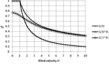
Asη2cannot be greater than 1, it is usually set to 1 whenU is smaller than 1 m s−1,

which generates a singular point forη2in function ofU as shown in Fig. 1.

Another solution consists in using the snowflake velocityV instead of the wind ve-locityU. V is classically composed of the wind velocity U and the terminal velocity Vt

(vertical velocity) of the snowflake according to Eq. (8):

5

V =U2+V_t20.5 (8)

As explained later,Vtis always greater than 1 m s−1, which means thatV is also greater

than 1 m s−1 in any case andη2can never be greater than 1. In the present study,η2

is estimated according to Eq. (9):

η2=V−0.5 (9)

10

The accretion efficiency factor η3 can be considered as a trigger: η3=1 means that

the accretion can start and/or continue andη3=0 means that snow cannot accrete.

As explained by Nygaard et al. (2013a), the liquid water fraction of the snow is the best parameter to determine if it can really accrete onto the collector. Unfortunately, that parameter is not measured routinely at weather stations.

15

According to Makkonen (1989), wet-bulb temperature Twb, which must be slightly

greater than 0◦C so as to allow flakes to be gently wet, is a good parameter to deter-mine if the snow can stick. Nygaard et al. (2013a) noticed that 95 % of the wet-snow cases occur at wet-bulb temperatures between 0 and 1◦C.

In this study, as in Makkonen and Wichura (2012), one part of the wet-snow accretion

20

criterion is Twb greater than −0.2 ◦

C. As Twb is not routinely recorded in all weather

stations, the following criterion Eq. (10) can be used to fix an equivalent lower limit to the relative humidity RH in function of the air temperatureTa:

(7)

NHESSD

2, 5139–5170, 2014

estimation

Title Page

Tables Figures

◭ ◮

Back Close

Full Screen / Esc

P

a

per

|

Discus

sion

P

a

per

|

Discussion

P

a

per

|

Discussion

P

a

per

If Twb is too high, precipitation may be rain instead of snow. Nygaard et al. (2013b)

noticed that the upper limit forTwb was slightly greater than 1 ◦

C in case of wet-snow events and proposed to use 1.2◦C as a practical upper limit. Makkonen (1989) pro-posed to use one of the Matsuo’s statistical criteria (1981) to determine the upper limit, which are quite equivalent to the previous one. In this study, the following Matsuo’s

5

criterion Eq. (11) is used:

RHup=39·(7.2−Ta)0.5 (11)

As noticed by Wakahama (1979), no wet-snow cases have been recorded for air tem-perature above 2◦C, which leads to the last criterion Eq. (12):

Ta≤2◦C (12)

10

As shown in Fig. 2, those three criteria draw a window in the plane formed by the air temperature and the relative humidity in whichη3can be set to 1.

2.3 Mass concentration of snowflakes in the air

One approach is to estimate the mass concentrationw from observed visibilityVm by

a formula presented in Makkonen (1989). That approach has not been chosen by the

15

authors as visibility has not been widely recorded in the past 25 years at su_fficiently many French weather stations.

Moreover, the same visibility may lead to very different snowfall rates, which are directly correlated to mass concentrationw through Eq. (13) whereVtis the snowflake

terminal velocity andP is the equivalent water precipitation intensity.

20

w=P Vt

(13)

(8)

NHESSD

2, 5139–5170, 2014

estimation

Title Page

Tables Figures

◭ ◮

Back Close

Full Screen / Esc

Discussion

P

a

per

|

Discus

sion

P

a

per

|

Discussion

P

a

per

|

Discussion

P

a

per

|

As the equivalent water precipitation intensity P is automatically recorded in many weather stations, Eq. (13) has been chosen by the authors to determinew.

Terminal velocity can depend on the riming degree of snowflakes (Böhm, 1999; Barthazy and Schefold, 2005), as well as temperature (Muramoto et al., 1993; Yuter et al., 2006; Zawadski et al., 2010) or height of snow system (Zawadski et al., 2010).

5

All studies show that wet-snow terminal velocity is bigger than 1 m s−1, which is gen-erally considered as suitable to describe dry-snow terminal velocity. Based on the work of Yuter et al. (2006) and Nygaard et al. (2013a) setVt to 1.7 m s−1, which is the value

used in this study as an average value for wet-snow terminal velocity.

In France, the intensity of precipitation is recorded by unshielded gauge

10

(Leroy, 2002), which means that the catch ratio of precipitation is smaller than 1 as soon as the wind is blowing (Goodison, 1978; Rasmussen et al., 2012).

Some catch ratio (CR in %) formulae are given in WMO report no.67 (1998) for snow (freezing temperature) or mixed precipitation recorded by unshielded gauges. As this study is about wet-snow fall, the following formula Eq. (14) intended for mixed

15

precipitation has been chosen:

CR=96.6+0.41·W2−9.84·W +5.95·Ta (14)

WhereW is the wind velocity at gauge height, which is roughly 70 % of the wind velocity

U recorded at 10 m a.g.l. according to the method proposed in the same WMO report. Therefore, the multiplicative correction factorcfor the intensity of precipitationP is:

20

c=100/CR (15)

2.4 Density of the accreted snow

Nygaard et al. (2013a) used a fixed value of 700 kg m−3, which was well correlated with Icelandic wet-snow case observation published by Elíasson et al. (2000) for windy events, i.e. wind velocity ranges from 10 to 25 m s−1.

(9)

NHESSD

2, 5139–5170, 2014

estimation

Title Page

Tables Figures

◭ ◮

Back Close

Full Screen / Esc

P

a

per

|

Discus

sion

P

a

per

|

Discussion

P

a

per

|

Discussion

P

a

per

As Strauss and Magnan (1985) noticed that wind velocity ranged from 0 to 10 m s−1 in more than 90 % of French wet-snow cases recorded between 1949 and 1982, that fixed value of 700 kg m−3cannot be used to study French wet-snow cases.

Deneau and Guillot (1984) estimated that the density of French wet-snow cases ranges from 300 to 500 kg m−3for wind velocity varying from 0 to 8 m s−1.

5

As this study is intended to determine 50 years return period wet-snow loads in France, the reasonable constant value of 400 kg m−3 proposed in ISO annex for wet-snow densityρsis adopted.

2.5 Shedding – end of event

In regions like French plains (below an altitude of 500 m), at the end of a wet-snow

10

fall, temperature usually increases and snow turns to rain, which initiates the shedding. This is not true for mountain areas where temperatures can drop after a wet-snow fall, which freezes the accretion.

In this study, the end of an event is characterized by a snow load that does not increase for at least 5 consecutive hours. That criterion is only available for French

15

plains or equivalent areas. In that case, accreted snow load is reset and the event is considered as over. Another criterion has to be elaborated for non equivalent areas as mountains.

3 Statistical aspects of the wet-snow load determination

3.1 Uncertainty estimation for one specific event

20

As soon as η3 is equal to 1, the wet-snow accretion load depends on two recorded

values, i.e.P andU, the duration, and four parameters, i.e.Vt,ρs,n(which leads toη2)

(10)

NHESSD

2, 5139–5170, 2014

estimation

Title Page

Tables Figures

◭ ◮

Back Close

Full Screen / Esc

Discussion

P

a

per

|

Discus

sion

P

a

per

|

Discussion

P

a

per

|

Discussion

P

a

per

|

In order to estimate the uncertainty of the model, the random aspect of those four parameters must be addressed.

A normal distribution of those parameters is assumed, considering that:

– Vt=1.7 m s−1,ρs=400 kg m−3,n=0.5 and CR calculated according to Eq. (14)

are reasonable mean values

5

– 10 % is the coe_fficient of variation for Vt (99 % of values can range from 1.3 to

2.1 m s−1

– 10 % is the coefficient of variation forρs (99 % of values can range from 300 to

500 kg m−3)

– 10 % is the coe_fficient of variation forn(95 % of values can range from 0.4 to 0.6)

10

– 15 % is the coefficient of variation for CR (from WMO report no.67)

With such an assumption, numerical simulations show that the distribution of the wet-snow load values for one given couple (P,U) and a duration is well represented by a gamma law whose median value is the value calculated according to the mean values of the four parameters.

15

The two classical parameters of that gamma law can easily be determined from its mean, which is 1.1 greater than its median value, and its coefficient of variation, which is 35 %. Those two estimations come from simulations of 20 000 cases, which are built with different couples (P,U) and different durations.

It can be practical to notice that 90 % confidence interval is easily determined using

20

the simple rule: [60 % of the median value–180 % of the median value].

For instance, when the calculation with the mean values of the parameters leads to 3.5 kg m−1 for one specific event, it can be reasonably considered that the wet-snow load is a random variable whose:

– median value is 3.5 kg m−1

(11)

NHESSD

2, 5139–5170, 2014

estimation

Title Page

Tables Figures

◭ ◮

Back Close

Full Screen / Esc

P

a

per

|

Discus

sion

P

a

per

|

Discussion

P

a

per

|

Discussion

P

a

per

– mean value is 1.1·3.5 kg m−1=3.8 kg m−1

– 90 % confidence interval is [0.6·3.5–1.8·3.5 kg m−1] or [2.1–6.3 kg m−1]

3.2 50 years return period wet-snow load determination

Data from weather stations that have been recorded for years are processed according

5

to the classical wet-snow accretion model and the parameterization proposed in this study.

In so doing, wet-snow events are isolated for each station and processed according to a POT method to evaluate the 50 years return period wet-snow loads of the weather station area.

10

Generalized Pareto Distribution (GPD) parameters of the POT method are evaluated according to the L-Moment method as proposed by Hosking (1990).

In so doing, what is called hereafter the “calculated value” of the 50 years return period wet-snow load is obtained.

In order to calculate the mean value and the 90 % confidence interval of the 50 years

15

return period wet-snow load, wet-snow load of each individual event is considered as being a random variable distributed according to the previously described gamma law. 10 000 numerical simulations for 4 different weather stations have showed that the 50 years return period wet-snow load is well represented by a normal law whose mean value is about 1.1 greater than the “calculated value” and coefficient of variation is

20

about 15 %.

It can be practical to notice that 90 % confidence interval is easily determined using the simple rule: [79 % of the “calculated value”–141 % of the “calculated value”].

Those precise values have been chosen because:

– they are quite consistent with the normal law described above

(12)

NHESSD

2, 5139–5170, 2014

estimation

Title Page

Tables Figures

◭ ◮

Back Close

Full Screen / Esc

Discussion

P

a

per

|

Discus

sion

P

a

per

|

Discussion

P

a

per

|

Discussion

P

a

per

|

– it can be shown that one and only one ISO Ice Class value (Table 4 of ISO 12494) can be found in such a confidence interval

One way to show that uniqueness is simply to notice that using the multiplicative factor 1.41/0.79=1.78 allows going from one ISO Ice Class value to the next as illustrated by the following examples:

5

– 1.6 kg m−1(R3) is equal to 1.78·0.9 kg m−1(R2)

– 8.9 kg m−1(R6) is equal to 1.78·5 kg m−1(R5)

For instance, when the “calculated value” of the 50 years return period wet-snow load for one station is 4 kg m−1, the mean 50 years return period load is 4.4 kg m−1 and the 90 % confidence interval of the 50 years return period wet-snow load is [3.2–

10

5.6 kg m−1].

The only IC value that can be found in this interval is 5 kg m−1. Therefore, it is sug-gested to consider ISO Ice Class R5 as being suitable for that example.

4 Application to the French wet-snow cases

4.1 French wet-snow design rules

15

Design rules to account for wet-snow loads established before 1950 are unknown. From a legal point of view, wind load and contraction due to freezing temperatures were the only meteorological resistance obligations.

From 1950 to 1985, with the creation of the national French company EDF, design rules became clearer. Describing these rules in terms of ISO and its reference collector,

20

it can be considered that:

(13)

NHESSD

2, 5139–5170, 2014

estimation

Title Page

Tables Figures

◭ ◮

Back Close

Full Screen / Esc

P

a

per

|

Discus

sion

P

a

per

|

Discussion

P

a

per

|

Discussion

P

a

per

– others plains were concerned by loads of 2 kg m−1

– mountains were concerned by loads of 5 kg m−1 or even 10 kg m−1 of accreted snow or rime

In 1987, due to some successive and memorable damageable wet-snow events, design rules were modified as follows:

5

– all plains were concerned by 2 kg m−1

– specific plains in the south part of the country were concerned by 5 kg m−1

– design rules in mountain area were unchanged

Since 1971, French accretion design rules have been described according to a thick-ness of accretion (snow, rime or glaze), i.e. 2, 4 or 6 cm, associated to a unique density

10

of 600 kg m−3, which are the equivalent of respectively 2, 5 and 10 kg m−1onto the ISO reference collector.

For pole and lattice tower design, symmetric and asymmetric ice loads on conductors combined with small wind loads (180 Pa on rimed conductors) are taken into account.

Those design rules have never been changed for new overhead lines since 1987.

15

It is important to underline the fact that all the lines designed according to 5 kg m−1 (4 cm of accreted snow of density 600 kg m−3) have never been damaged by any wet-snow events in plains since their construction.

4.2 Chosen weather stations

The model described in Sect. 2 and the statistical approach described in Sect. 3 have

20

been used with recorded data from 82 French weather stations well distributed all over the country.

Those stations have been selected according to the four following criteria:

(14)

NHESSD

2, 5139–5170, 2014

estimation

Title Page

Tables Figures

◭ ◮

Back Close

Full Screen / Esc

Discussion

P

a

per

|

Discus

sion

P

a

per

|

Discussion

P

a

per

|

Discussion

P

a

per

|

– 25 years period is considered by the authors as a minimum to estimate 50 years return period loads

– It is assumed that 25 year period is short enough to avoid any distortion due to potential e_ffects of climatic changes

2. Altitude smaller than 500 m

5

– Above 500 m, the criterion chosen to consider that the event is over (shed-ding) cannot be considered as being usable (see Sect. 2.5)

– The main focus of this study is the wet-snow loads in French plains at low altitude, which represent about 80 % of the territory

3. Normal environmental situation

10

– Stations located on areas highly influenced by orography have not been cho-sen (for instance stations upon cliffs)

4. Good data quality

– Air temperature, relative humidity, intensity of precipitation and wind velocity have to be recorded every three hours or less

15

5 others stations at an altitude greater than 500 m, i.e. Aurillac (640 m), Millau (720 m), Le Puy (833 m), Bourg-St-Maurice (868 m) and Embrun (876 m) are added to this study in order to test the model parameterization in areas slightly above 500 m.

4.3 Results of the calculation for the last 25 winters

According to the data of the 87 selected weather stations, 170 events with a load equal

20

to or greater than 1 kg m−1were simulated by the model proposed in Sect. 2.

(15)

NHESSD

2, 5139–5170, 2014

estimation

Title Page

Tables Figures

◭ ◮

Back Close

Full Screen / Esc

P

a

per

|

Discus

sion

P

a

per

|

Discussion

P

a

per

|

Discussion

P

a

per

All those noticeable events have been well simulated by the model, i.e. good local-izations, good dates and calculated loads consistent with the real damages taking into account the overhead line design as described in Sect. 4.1.

When an event cannot be associated with more than one collapsed pole or tower or when an event concerns a small area, no internal report is produced. Nevertheless,

5

the event is recorded in a database, which is used in the following.

As explained in Sect. 4.2, 5 out of the 87 stations of that study (6 %) are located at an altitude greater than 500 m. Those stations are concerned by 37 out of the 170 events (22 %) with a load equal to or greater than 1 kg m−1. Few of those 37 events can be related to real damages because the design loads in these kinds of regions have

10

already taken into account heavy wet-snow and rime loads for a long time, i.e. 5 or even 10 kg m−1.

The remaining 133 events concern plains at altitude below 500 m, where wet-snow loads have not been taken into account in the design of overhead lines or have been taken into account according to a value of about 2 kg m−1.

15

Those 133 simulated events have been distributed into 4 classes: more than 3 kg m−1 (14 cases), between 2 and 3 kg m−1 (27 cases), between 1.5 and 2 kg m−1 (25 cases) and between 1 and 1.5 kg m−1(67 cases).

When available, present weather codes (PW) were used to check if the criterion proposed in Sect. 2.2 was able to select real snow cases. In 37 out of 133 cases

20

(28 %), PW showed that precipitation was rain or a mixture of rain (code 60 to 65) and snow (code 70 to 75), which means that it is likely that the precipitation was too wet to generate real wet-snow accretion events. That assumption is verified as no associated real events were found in the database. In that way, the model can be considered as being slightly conservative.

25

(16)

NHESSD

2, 5139–5170, 2014

estimation

Title Page

Tables Figures

◭ ◮

Back Close

Full Screen / Esc

Discussion

P

a

per

|

Discus

sion

P

a

per

|

Discussion

P

a

per

|

Discussion

P

a

per

|

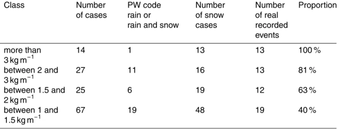
In the remaining 96 cases, 57 real recorded events (60 %) could be associated with calculated loads greater than 1 kg m−1. Details are summarized in Table 1.

As expected, when the calculated load is greater than 2 kg m−1, which is the “normal” design load in plains, the proportion of real recorded events that can be found in the database is important (90 %). Worst simulated events, i.e. calculated loads greater than

5

5 kg m−1, concern generally real recorded events with collapsed towers and poles. For calculated loads between 1 and 2 kg m−1, that proportion is smaller (46 %) but still consistent with the fact that:

– Calculated loads are median values as explained in Sect. 3.1

– Some overhead lines designed before 1987 were not supposed to resist loads up

10

to 2 kg m−1

Even if a calculated load is not sufficient to generate damage, it must be kept in order to have enough cases to calculate the 50 years return period wet-snow loads according to the POT method as presented in the next section.

4.4 50 years return period wet-snow loads according to POT method

15

For each weather station, simulated wet-snow loads have been calculated according to the model described in Sect. 2.

For instance, 241 loads have been calculated according to 187 327 meteorological records in 25 years for Lille station in the north of France.

Among those 241 loads represented on Fig. 3, only 22 are greater than a threshold

20

of 0.3 kg m−1.

Using L-moment method as explained in Sect. 3.2, the Generalized Pareto Distribu-tion (GPD) parameters of the POT method can be calculated and the 50 years return period load determined.

In the case of Lille, that value is 2.6 kg m−1, which means that, according to the

prac-25

(17)

NHESSD

2, 5139–5170, 2014

estimation

Title Page

Tables Figures

◭ ◮

Back Close

Full Screen / Esc

P

a

per

|

Discus

sion

P

a

per

|

Discussion

P

a

per

|

Discussion

P

a

per

and the 90 % confidence interval calculated is [2–3.6 kg m−1]. Consequently, the ISO IC for Lille is R4.

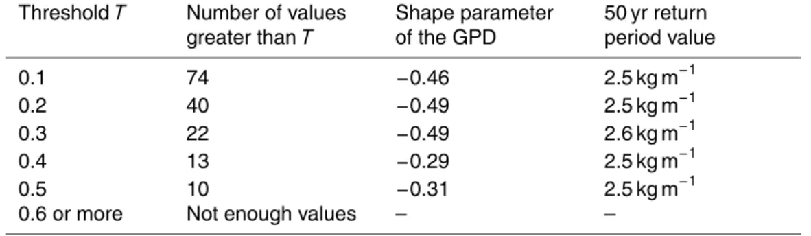
The influence of the threshold is presented in Table 2. It can be noticed that:

– The 50 years return period value is very stable

– The shape parameter of the GPD is always in the range [−0.5–0], which is the

5

optimal range according to Hosking (1990)

In this study, the optimal choice of the threshold value for each station had generally led to a number of selected values arround 25.

The case of Lille is also very interesting because of the highest calculated value (3.2 kgm−1) recorded in March 2012. As the 50 years return period determination is

10

highly influenced by the highest value, a special attention must be paid to that case. In two thirds of the west and north part of the country roughly located between the Atlantic side and the moutain areas, such a value, which has been associated with a real noticeable event (one 225 kV collapsed tower and a dozen of 400 kV damaged towers) is more than extremely rare.

15

For Lille station, the second biggest value is only 1.4 kg m−1, which is less than half the biggest value.

In one background document of EN 1991-1-3, i.e. the Final Report produced by San-paolesi (1998) about snow load determination, one criterion for identifying “exceptional load” values is expressed as:

20

If the ratio of the largest load value to the characteristic load (50 years return period load) determined without the inclusion of that value is greater than 1.5 then the largest load value shall be treated as an exceptional value (and not used in the determination of the 50 years return period value).

In the case of Lille, the mean 50 years return period load determined without the largest

25

(18)

NHESSD

2, 5139–5170, 2014

estimation

Title Page

Tables Figures

◭ ◮

Back Close

Full Screen / Esc

Discussion

P

a

per

|

Discus

sion

P

a

per

|

Discussion

P

a

per

|

Discussion

P

a

per

|

be excluded and the new 90 % confidence interval could be [1.2–2.4 kg m−1] and the new ISO IC could be R3.

It is suggested to use the above criterion only when the exceptional aspect of the value can be checked, i.e. according to a real event database, as in the case of the exceptional Lille event of March 2012.

5

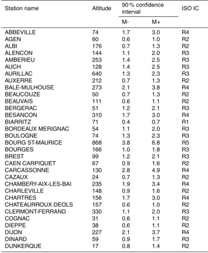
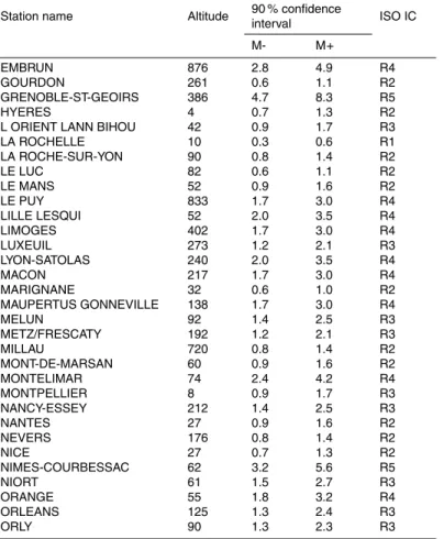
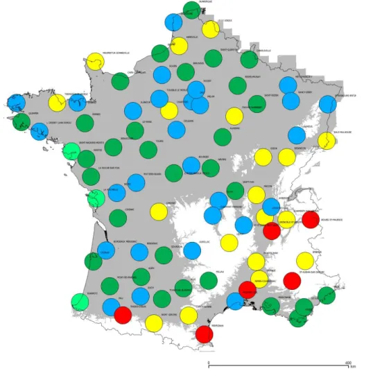
For the 87 French weather stations, each ISO IC has been calculated (Table 3) with-out excluding the largest value, even when the criterion evocated above was positive. Results are presented in Fig. 4.

Each station is at the center of a circle of 50 km in diameter and it may be not prudent to extrapolate what is calculated according to the data recorded at one specific station

10

outside its associated circle, especially in the case of different valleys in mountain ar-eas.

4.5 Comparisons with previous winter wet-snow events

Real cases that affected the transmission network before 1987 are represented in an old internal EDF document produced by Mazingarbe (1987). All cases but one

hap-15

pened in the mountains area or in the plains of the south part of the country as shown in Fig. 5.

As expected, few events are recorded in the Alps as overhead lines have already been designed with heavy loads in this area for many years.

In the West part of the Mediterranean coast (Perpignan) severe events happened in

20

1981 and 1986, which is consistent with what can be estimated according to the data of the last 25 winters:

– another noticeable event (many collapsed towers) happened in the same area in 1992

– one of the biggest 50 years return period load in France for Perpignan (ISO IC R5)

(19)

NHESSD

2, 5139–5170, 2014

estimation

Title Page

Tables Figures

◭ ◮

Back Close

Full Screen / Esc

P

a

per

|

Discus

sion

P

a

per

|

Discussion

P

a

per

|

Discussion

P

a

per

In the region of the Rhône Valley, severe events also happened in 1970, 1974 and 1982. As expected, many stations along that valley are concerned by an important ISO IC, i.e. R4 and R5, compared to the west or north part of France, i.e. mainly R1, R2 or R3.

The same conclusions can be drawn for the foothills of the Pyreneans:

5

– a lot of events were recorded before 1987

– a very noticeable event in January 1997 in the same area (damaged and broken earth-wires and conductors, damaged or collapsed poles or towers)

– one of the biggest 50 years return period load in France for Tarbes (ISO IC R5)

Thus, it can be considered that the analysis of the last 25 winters, according to the

10

model proposed in Sect. 2, is consistent with what happened during previous winters.

5 Conclusions

Two modifications of the parameterization proposed by Nygaard et al. (2013a) for the conventional cylindrical wet-snow accretion model have been introduced:

– reduced mean value of the accretion density more adapted to the small wind

15

velocity during French wet-snow precipitations

– estimation of mass concentration of snowflakes in the atmosphere according to the wind-effect corrected intensity of precipitation recorded in French weather sta-tions

Taking into account the original wet-snow load design of French overhead lines, that

20

(20)

NHESSD

2, 5139–5170, 2014

estimation

Title Page

Tables Figures

◭ ◮

Back Close

Full Screen / Esc

Discussion

P

a

per

|

Discus

sion

P

a

per

|

Discussion

P

a

per

|

Discussion

P

a

per

|

Then, for each station, all simulated events during the last 25 winters have been used to estimate the 90 % confidence intervals of 50 years return period wet-snow loads. As only one ISO IC value could be found in each interval, a unique ISO IC has been determined this way for each station.

The distribution of the 87 wet-snow loads on a French map has shown that

ar-5

eas concerned by heavy characteristic loads had already been affected by noticeable events that happened before the last 25 winters used to calculate the 87 characteristic 50 years return period loads.

Nevertheless, it is prudent to underline the fact that the 50 years return period wet-snow load calculated at a specific weather station can only be considered as being

10

available in the vicinity of that station, i.e. in a circle of about 50 km in diameter centered at the station.

Thus, the method described in that paper can essentially be used to check that a wet-snow design load map, based on experience or on long-term applications with positive results, can be effectively related to 50 years return period wet-snow loads in

15

the vicinity of many weather stations.

References

Admirat, P., Sakamoto, Y., and De Goncourt, B.: Calibration of a snow accumulation model based on actual cases in Japan and France, Proc. 4th International Workshop on Atmo-spheric Icing of Structures, Paris, France, 5–7 September 1988.

20

Barthazy, E. and Schefold, R.: Fall velocity of snowflakes of different riming degree and crystal types, Atmos. Res., 82, 391–398, 2006.

Böhm, H. P.: A general equation for the terminal fall speed of solid hydrometeors, J. Atmos. Sci., 46, 2419–2427, 1989.

Deneau, V. and Guillot, P.: Wet-snow accretion on power lines: cartographic examination of

25

(21)

NHESSD

2, 5139–5170, 2014

estimation

Title Page

Tables Figures

◭ ◮

Back Close

Full Screen / Esc

P

a

per

|

Discus

sion

P

a

per

|

Discussion

P

a

per

|

Discussion

P

a

per

Elíasson, A. J., Thorsteins, E., and Ólafsson H.: Study of wet-snow events on the south coast of Iceland, Proc. 9th International Workshop on Atmospheric Icing of Structures, Chester, England, 5–8 June 2000.

Elíasson, A. J., Ágústsson, H., Hannesson, G. M., and Thorsteins, E.: Modeling wet-snow accretion: Comparison of cylindrical model to field measurements, Proc. 15th International

5

Workshop on Atmospheric Icing of Structures, Newfoundland and Labrador, Canada, 8–13 September 2013.

EN 50341-1: Overhead electrical lines exceeding AC 1 kV – Part 1: General requirements – Common specifications, European Committee for Electrotechnical Standardization, 2012. Goodison, B. E.: Accuracy of Canadian snow gage measurements, J. Appl. Meteorol., 17,

10

1542–1548, 1978.

Goodison, B. E., Louie, P. Y. T., and Yang, D.: Report no.67: WMO solid precipitation measure-ment intercomparison – Final report, World Meteorological Organization, Geneva, 1998. Hosking, J. R. M.: L-moments: analysis and estimation of distributions using linear

combina-tions of order statistics, J. Roy. Stat. Soc. B. Met., 52, 105–124, 1990.

15

ISO 12494: Atmospheric icing of structures, International Standard Organization, 2001. Leroy, M.: La mesure au sol de la température et des précipitations, La Météorologie, 39, 52–

56, 2002 (in French).

Makkonen, L.: Estimation of wet-snow accretion on structures, Cold. Reg. Sci. Technol., 17, 83–88, 1989.

20

Makkonen, L. and Wichura, B.: Simulating wet-snow loads on power line cables by a simple model, Cold. Reg. Sci. Technol., 61, 73–81, 2010.

Matsuo, T., Sasyo, Y., and Sato, Y.: Relationship between types of precipitation on the ground and surface meteorological elements, J. Meteorol. Soc. Jpn., 54, 462–475, 1981.

Mazingarbe, E.: Lignes aériennes – Tenue aux surcharges importantes d’origine

25

météorologique – Givre, verglas, neige collante – Zones à risques, internal document of Electricité de France, Paris, 1987 (in French).

Muramoto, K. I., Matsuura, K., Harimaya, T., and Endoh, T.: A computer database for falling snowflakes, Ann. Glaciol., 18, 11–16, 1993.

Nygaard, B. E., Ágústsson, H., and Somfalvi-Tóth, K.: Modeling wet-snow accretion on power

30

(22)

NHESSD

2, 5139–5170, 2014

estimation

Title Page

Tables Figures

◭ ◮

Back Close

Full Screen / Esc

Discussion

P

a

per

|

Discus

sion

P

a

per

|

Discussion

P

a

per

|

Discussion

P

a

per

|

Nygaard, B. E., Fikke, S. M., Wareing, B., Seierstad, I. A., and Horsman, D.: The development of new maps for design ice loads for Great Britain, Proc. 15th International Workshop on Atmo-spheric Icing of Structures, Newfoundland and Labrador, Canada, 8–13 September 2013b. Rasmussen, R. M., Vivekanandan, J., Cole, J., Myers, B., and Masters, C.: The estimation of

snowfall rate using visibility, J. Appl. Meteorol., 38, 1542–1563, 1998.

5

Rasmussen, R., Baker, B., Kochendorfer, J., Myers, T., Landolt, S., Fisher, A., Black, J., Theri-ault, J., Kucera, P., Gochis, D., Smith, C., Nitu, R., Hall, M., Cristanelli, S., and Gutmann, E.: How well are we measuring snow? The NOAA/FAA/NCAR winter precipitation test bed, B. Am. Meteorol. Soc., 93, 811–829, 2012.

Sanpaolesi, L.: Phase 1 Final Report to the European Commission, Scientific Support Activity

10

in the Field of Structural Stability of Civil Engineering Works: Snow Loads, Department of Structural Engineering, University of Pisa, 1998.

Strauss, B. and Magnan, J.: Cartographie des risques de givre, verglas, neige collante à partir du fichier d’observations synoptiques de la météorologie nationale, Proc. Les Lignes aéri-ennes face à l’environnement climatique, Société des électriciens des électrotechniciens et

15

des radioélectriciens, Gif-sur-Yvette, 25 April 1985 (in French).

Wakahama, G.: Experimental studies of snow accretion on electric lines developed in a strong wind, J. Natural Disast. Sci., 1, 21–33, 1979.

Yuter, S. E., Kingsmill, D. E., Nance, L. B., and Löffler-Mang, M.: Observations of precipitation size and fall speed characteristics within coexisting rain and wet-snow, J. Appl. Meteorol.

20

Clim., 45, 1450–1464, 2006.

(23)

NHESSD

2, 5139–5170, 2014

estimation

Title Page

Tables Figures

◭ ◮

Back Close

Full Screen / Esc

P

a

per

|

Discus

sion

P

a

per

|

Discussion

P

a

per

|

Discussion

P

a

per

Table 1.Study of the 133 cases of calculated loads greater than 1 kg m−1.

Class Number of cases

PW code rain or rain and snow

Number of snow cases

Number of real recorded events

Proportion

more than 3 kg m−1

14 1 13 13 100 %

between 2 and 3 kg m−1

27 11 16 13 81 %

between 1.5 and 2 kg m−1

25 6 19 12 63 %

between 1 and 1.5 kg m−1

(24)

NHESSD

2, 5139–5170, 2014

estimation

Title Page

Tables Figures

◭ ◮

Back Close

Full Screen / Esc

Discussion

P

a

per

|

Discus

sion

P

a

per

|

Discussion

P

a

per

|

Discussion

P

a

per

|

Table 2.Study of the 50 years return period load for Lille in function of the threshold choice.

ThresholdT Number of values greater thanT

Shape parameter of the GPD

50 yr return period value

0.1 74 −0.46 2.5 kg m−1

0.2 40 −0.49 2.5 kg m−1

0.3 22 −0.49 2.6 kg m−1

0.4 13 −0.29 2.5 kg m−1

0.5 10 −0.31 2.5 kg m−1

(25)

NHESSD

2, 5139–5170, 2014

estimation

Title Page

Tables Figures

◭ ◮

Back Close

Full Screen / Esc

P

a

per

|

Discus

sion

P

a

per

|

Discussion

P

a

per

|

Discussion

P

a

per

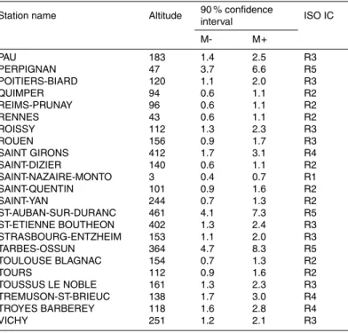
Table 3.87 French weather stations with their names, altitudes, 90 % confidence intervals and ISO IC.

Station name Altitude 90 % confidence

interval ISO IC

M- M+

ABBEVILLE 74 1.7 3.0 R4

AGEN 60 0.6 1.0 R2

ALBI 176 0.7 1.3 R2

ALENCON 144 1.1 2.0 R3

AMBERIEU 253 1.4 2.5 R3

AUCH 128 1.4 2.5 R3

AURILLAC 640 1.3 2.3 R3

AUXERRE 212 0.7 1.3 R2

BALE-MULHOUSE 273 2.1 3.8 R4

BEAUCOUZE 50 0.7 1.3 R2

BEAUVAIS 111 0.6 1.1 R2

BERGERAC 51 1.2 2.1 R3

BESANCON 310 1.7 3.0 R4

BIARRITZ 71 0.4 0.7 R1

BORDEAUX MERIGNAC 54 1.1 2.0 R3

BOULOGNE 74 1.3 2.3 R3

BOURG ST-MAURICE 868 3.8 6.8 R5

BOURGES 166 1.0 1.8 R3

BREST 99 1.2 2.1 R3

CAEN CARPIQUET 67 0.9 1.6 R2

CARCASSONNE 130 2.8 4.9 R4

CAZAUX 24 0.7 1.3 R2

CHAMBERY-AIX-LES-BAI 235 1.9 3.4 R4

CHARLEVILLE 148 0.9 1.6 R2

CHARTRES 156 1.7 3.0 R4

CHATEAURROUX DEOLS 157 0.6 1.0 R2

CLERMONT-FERRAND 330 1.1 2.0 R3

COGNAC 31 0.6 1.1 R2

DIEPPE 38 0.6 1.1 R2

DIJON 227 2.1 3.7 R4

DINARD 59 0.9 1.7 R3

(26)

NHESSD

2, 5139–5170, 2014

estimation

Title Page

Tables Figures

◭ ◮

Back Close

Full Screen / Esc

Discussion

P

a

per

|

Discus

sion

P

a

per

|

Discussion

P

a

per

|

Discussion

P

a

per

|

Table 3.Continued.

Station name Altitude 90 % confidence

interval ISO IC

M- M+

EMBRUN 876 2.8 4.9 R4

GOURDON 261 0.6 1.1 R2

GRENOBLE-ST-GEOIRS 386 4.7 8.3 R5

HYERES 4 0.7 1.3 R2

L ORIENT LANN BIHOU 42 0.9 1.7 R3

LA ROCHELLE 10 0.3 0.6 R1

LA ROCHE-SUR-YON 90 0.8 1.4 R2

LE LUC 82 0.6 1.1 R2

LE MANS 52 0.9 1.6 R2

LE PUY 833 1.7 3.0 R4

LILLE LESQUI 52 2.0 3.5 R4

LIMOGES 402 1.7 3.0 R4

LUXEUIL 273 1.2 2.1 R3

LYON-SATOLAS 240 2.0 3.5 R4

MACON 217 1.7 3.0 R4

MARIGNANE 32 0.6 1.0 R2

MAUPERTUS GONNEVILLE 138 1.7 3.0 R4

MELUN 92 1.4 2.5 R3

METZ/FRESCATY 192 1.2 2.1 R3

MILLAU 720 0.8 1.4 R2

MONT-DE-MARSAN 60 0.9 1.6 R2

MONTELIMAR 74 2.4 4.2 R4

MONTPELLIER 8 0.9 1.7 R3

NANCY-ESSEY 212 1.4 2.5 R3

NANTES 27 0.9 1.6 R2

NEVERS 176 0.8 1.4 R2

NICE 27 0.7 1.3 R2

NIMES-COURBESSAC 62 3.2 5.6 R5

NIORT 61 1.5 2.7 R3

ORANGE 55 1.8 3.2 R4

ORLEANS 125 1.3 2.4 R3

(27)

NHESSD

2, 5139–5170, 2014

estimation

Title Page

Tables Figures

◭ ◮

Back Close

Full Screen / Esc

P

a

per

|

Discus

sion

P

a

per

|

Discussion

P

a

per

|

Discussion

P

a

per

Table 3.Continued.

Station name Altitude 90 % confidence_interval ISO IC

M- M+

PAU 183 1.4 2.5 R3

PERPIGNAN 47 3.7 6.6 R5

POITIERS-BIARD 120 1.1 2.0 R3

QUIMPER 94 0.6 1.1 R2

REIMS-PRUNAY 96 0.6 1.1 R2

RENNES 43 0.6 1.1 R2

ROISSY 112 1.3 2.3 R3

ROUEN 156 0.9 1.7 R3

SAINT GIRONS 412 1.7 3.1 R4

SAINT-DIZIER 140 0.6 1.1 R2

SAINT-NAZAIRE-MONTO 3 0.4 0.7 R1

SAINT-QUENTIN 101 0.9 1.6 R2

SAINT-YAN 244 0.7 1.3 R2

ST-AUBAN-SUR-DURANC 461 4.1 7.3 R5

ST-ETIENNE BOUTHEON 402 1.3 2.4 R3

STRASBOURG-ENTZHEIM 153 1.1 2.0 R3

TARBES-OSSUN 364 4.7 8.3 R5

TOULOUSE BLAGNAC 154 0.7 1.3 R2

TOURS 112 0.9 1.6 R2

TOUSSUS LE NOBLE 161 1.3 2.3 R3

TREMUSON-ST-BRIEUC 138 1.7 3.0 R4

TROYES BARBEREY 118 1.6 2.8 R4

(28)

NHESSD

2, 5139–5170, 2014

estimation

Title Page

Tables Figures

◭ ◮

Back Close

Full Screen / Esc

Discussion

P

a

per

|

Discus

sion

P

a

per

|

Discussion

P

a

per

|

Discussion

P

a

per

|

 Figure 1.Sticking e_fficiency factorη2whenVt=1.7 m s−

1

(29)

NHESSD

2, 5139–5170, 2014

estimation

Title Page

Tables Figures

◭ ◮

Back Close

Full Screen / Esc

P

a

per

|

Discus

sion

P

a

per

|

Discussion

P

a

per

|

Discussion

P

a

per



(30)

NHESSD

2, 5139–5170, 2014

estimation

Title Page

Tables Figures

◭ ◮

Back Close

Full Screen / Esc

Discussion

P

a

per

|

Discus

sion

P

a

per

|

Discussion

P

a

per

|

Discussion

P

a

per

|

(31)

NHESSD

2, 5139–5170, 2014

estimation

Title Page

Tables Figures

◭ ◮

Back Close

Full Screen / Esc

P

a

per

|

Discus

sion

P

a

per

|

Discussion

P

a

per

|

Discussion

P

a

per

(32)

NHESSD

2, 5139–5170, 2014

estimation

Title Page

Tables Figures

◭ ◮

Back Close

Full Screen / Esc

Discussion

P

a

per

|

Discus

sion

P

a

per

|

Discussion

P

a

per

|

Discussion

P

a

per

|