www.hydrol-earth-syst-sci.net/19/4441/2015/ doi:10.5194/hess-19-4441-2015
© Author(s) 2015. CC Attribution 3.0 License.
SACRA – a method for the estimation of global high-resolution crop
calendars from a satellite-sensed NDVI
S. Kotsuki1and K. Tanaka2
1RIKEN Advanced Institute for Computational Science, Kobe, Japan 2Disaster Prevention Research Institute, Kyoto University, Kyoto, Japan Correspondence to: S. Kotsuki ([email protected])
Received: 22 December 2014 – Published in Hydrol. Earth Syst. Sci. Discuss.: 29 January 2015 Revised: 5 October 2015 – Accepted: 15 October 2015 – Published: 5 November 2015
Abstract. To date, many studies have performed numerical estimations of biomass production and agricultural water de-mand to understand the present and future supply–dede-mand relationship. A crop calendar (CC), which defines the date or month when farmers sow and harvest crops, is an essential in-put for the numerical estimations. This study aims to present a new global data set, the SAtellite-derived CRop calendar for Agricultural simulations (SACRA), and to discuss advan-tages and disadvanadvan-tages compared to existing census-based and model-derived products. We estimate global CC at a spa-tial resolution of 5 arcmin using satellite-sensed normalized difference vegetation index (NDVI) data, which corresponds to vegetation vitality and senescence on the land surface. Us-ing the time series of the NDVI averaged from three con-secutive years (2004–2006), sowing/harvesting dates are es-timated for six crops (temperate-wheat, snow-wheat, maize, rice, soybean and cotton). We assume time series of the NDVI represent the phenology of one dominant crop and estimate CCs of the dominant crop in each grid. The dom-inant crops are determined using harvested areas based on census-based data. The cultivation period of SACRA is iden-tified from the time series of the NDVI; therefore, SACRA considers current effects of human decisions and natural dis-asters. The difference between the estimated sowing dates and other existing products is less than 2 months (< 62 days) in most of the areas. A major disadvantage of our method is that the mixture of several crops in a grid is not considered in SACRA. The assumption of one dominant crop in each grid is a major source of discrepancy in crop calendars be-tween SACRA and other products. The disadvantages of our approach may be reduced with future improvements based on finer satellite sensors and crop-type classification studies
to consider several dominant crops in each grid. The compar-ison of the CC also demonstrates that identification of wheat type (sowing in spring or fall) is a major source of error in global CC estimations.
1 Introduction
Recent population growth has increased biomass demand significantly, and humans have expanded cropland globally. Agriculture occupies more than 70 % of world water us-age and has a large impact on the water cycle (Rost et al., 2008). Consequently, simulations of biomass production and agricultural water demand are necessary to understand the present and future supply–demand relationship. To date, many studies have estimated biomass accumulation (Fischer et al., 2000; Tan and Shibasaki, 2003; Stehfest et al., 2007) and agriculture water demand (Döll et al., 2002; Hanasaki et al., 2008; Rockström et al., 2009; Siebert and Döll, 2010; Pokrel et al., 2012). Those studies estimated biomass pro-duction and agricultural water demand with numerical mod-els using meteorological forcing data and land surface pa-rameters. A crop calendar (CC) is an essential input to esti-mate biomass production and agricultural water demand ac-curately with those numerical models. CCs define the date or month when farmers sow and harvest crops. There are three major approaches to developing CC data sets: census-based; model-based; and Earth observation-based.
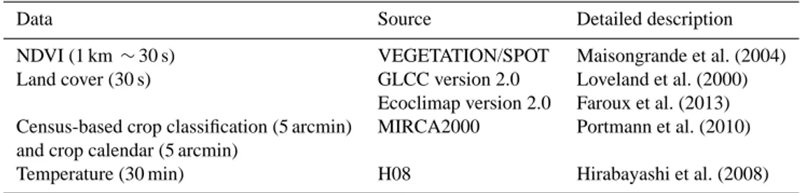
Table 1. Characteristics and sources of the four global input data sets.
Data Source Detailed description NDVI (1 km∼30 s) VEGETATION/SPOT Maisongrande et al. (2004) Land cover (30 s) GLCC version 2.0 Loveland et al. (2000)
Ecoclimap version 2.0 Faroux et al. (2013) Census-based crop classification (5 arcmin) MIRCA2000 Portmann et al. (2010) and crop calendar (5 arcmin)
Temperature (30 min) H08 Hirabayashi et al. (2008)
Table 2. List of crops. Checkmarks denote crops used for (a) estimation of crop calendar and (b) comparison of cropping intensity.
ID Crop name (a) Calendar (b) Intensity ID Crop name (a) Calendar (b) Intensity 1 Temperate-wheat X X 10 Millet X
2 Snow-wheat X X 11 Oil palm X
3 Maize X X 12 Potato X
4 Rice X X 13 Rapeseed X
5 Soybean X X 14 Rye X
6 Cotton X 15 Sorghum X
7 Barley X 16 Sugarcane X
8 Cassava X 17 Sunflower X
9 Groundnuts X
Figure 1. Data processing scheme for the production of the global
satellite-derived crop calendar (SACRA). The bold numbers inside the boxes indicate the subsections in this paper where the different processing steps are described. The numbers outside the boxes in-dicate the spatial resolution of the respective data sets. The top four boxes indicate input data (Table 1), and the other boxes indicate the results from our data processes.
States Department of Agriculture (USDA). The census-based CC products are represented by MIRCA2000 (Portmann et al., 2010; Monthly Irrigated and Rain-fed Crop Areas around the year 2000) and Sacks et al. (2010). The census-based products have the advantage of high reliability in regions that have sufficient census data. However, they also have the disadvantage of low reliability in regions that have no
cen-sus data. Additionally, the spatial resolution of cencen-sus-based products is limited because of the sampling scheme (Port-mann et al., 2010). Because only one CC is defined per ad-ministrative unit for each crop, differences in CCs for the same administrative unit are not considered.
Model-based approaches generate CCs using crop growth models. These models simulate crop growth based on mete-orological forcing data such as temperature, solar radiation, and soil moisture. In particular, accumulated temperature is widely used to indicate phenological progress. Hanasaki et al. (2008) estimated global CCs for several crops using the Soil and Water Integrated Model (SWIM; Krysanova et al., 2000). Waha et al. (2012) simulated the sowing dates of major annual crops based on climatic conditions and crop-specific temperature requirements. The crop growth models have the advantage of accurate crop growth simulation in cases of well-calibrated parameters. However, proper cali-bration is difficult in areas where observation data are insuf-ficient. Additionally, the crop growth model, being based on environmental processes, is of limited accuracy with respect to the identification of sowing dates, because the sowing date is heavily affected by human decisions.
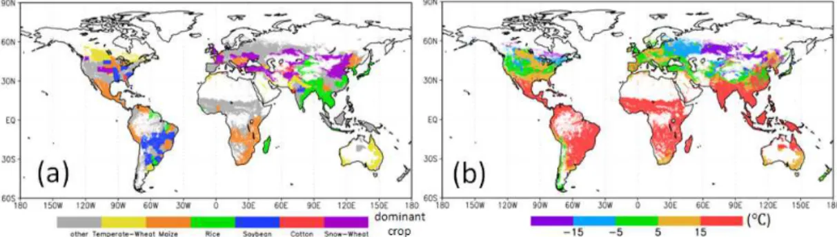
Figure 2. Global distribution of (a) dominant crops in SACRA, and (b) minimum monthly averaged temperature (◦C) during the cultivation
period of the dominant crops. Both panels represent the dominant crop in the major cultivation season.
of satellite-derived data is its spatial resolution (less than 1 km). However, a few studies have estimated global CCs with satellite-derived data. Yorozu et al. (2005) estimated a global CC using the normalized difference vegetation index (NDVI), but they did not compare their results to other global CC data sets.
In this paper, we present a new global data set, the SAtellite-derived CRop calendar for Agricultural simulations (SACRA). Using satellite-sensed NDVI data, we estimate the global CC at a spatial resolution of 5 arcmin (∼9.2 km at the Equator). This study aims to develop a high-resolution and highly accurate CC product by combining the satellite-derived NDVI with a census-based product. We also aim to discuss the advantages and disadvantages of our satellite-derived CC, compared to existing census-based and model-derived products. The products are available for download at http://data-assimilation.jp/opendata/sacra/sacra_des.html.
2 Materials and methods
This section describes the methods applied to produce SACRA according to a defined data processing scheme (Fig. 1). SACRA is produced from four different data sets: time series of the NDVI; land cover data; reanalysis temper-ature data; and census-based agricultural data (Table 1). This study estimates the CC for six crops (temperate-wheat, snow-wheat, rice, maize, soybean, and cotton) that are widely culti-vated around the world (Table 2a). We treat temperate-wheat and snow-wheat separately because our method is unsuitable for estimating the sowing date in grid areas where the surface is covered by snow during the cultivating period (e.g., Russia and North China; see Sect. 2.3 for details).
The following subsections describe identification of the dominant crop and census-based CC (Sect. 2.1), vegetation indices (Sect. 2.2), estimation of global crop calendar (first estimation; Sect. 2.3) and the SACRA data sets (Sect. 2.4).
2.1 Dominant crop and census-based sowing/harvesting data
Firstly, we identify the dominant crop at a spatial resolution of 5 arcmin using MIRCA2000. The grid of SACRA is set to that of MIRCA2000. Portmann et al. (2010) compiled ir-rigated and rain-fed areas of 26 crop types at a spatial reso-lution of 5 arcmin (cf. Table 4 in Portmann et al., 2010). In other words, we can obtain 52 classes of crop areas at each grid (i.e., both irrigated and rain-fed areas of 26 crop types). Their crop calendars in major and second cultivation seasons are also defined in MIRCA2000. Since our method cannot consider the mixture of several crops in a grid (see Sect. 2.2.2 for details), we consider only one dominant crop in each grid. We define the dominant crop in the major cultivation season as that which has the maximal harvested area in the grid, out of 52 possible crops (considering rain-fed and irrigated areas separately; cf. Appendix I in Portmann, 2011). If more than two crops have identical harvested areas, the early order of the crops is chosen to be the dominant crop (e.g., for irrigated wheat in India (Uttar Pradesh) with two identical areas with different cropping periods; cf. Table I-211 of Appendix I in Portmann, 2011). The dominant crop in the second cultiva-tion season is determined from those crops whose cultivacultiva-tion periods do not overlap more than 3 months with that of the dominant crop in the major cultivation season.
Secondly, we obtain the sowing and harvesting months of the dominant crop in both major and second cultivation sea-sons, using MIRCA2000. At each grid, we use the sowing and harvesting months. The census-based sowing and har-vesting months are used to calibrate crop calendar parame-ters in Sect. 2.3.
MIRCA2000-derived cultivating periods (from sowing month to harvest-ing month) and reanalysis temperature (Hirabayashi et al., 2008). Hirabayashi et al. (2008) compiled 3-hourly surface temperature data by statistical methods, the parameters of which had been obtained from available surface observa-tions. Here, we simply use the reanalyzed temperature of the nearest 30 arcmin grid from MIRCA2000’s 5 arcmin grids.
The resulting global distribution of dominant crops in SACRA in the major cultivation season is shown in Fig. 2a. The minimum monthly averaged temperature during the cul-tivation period of the dominant crop is shown in Fig. 2b. Regions showing the minimum monthly averaged tempera-tures below 5.0◦C in Fig. 2b are categorized as snow-wheat (purple) or other crops (grey) in Fig. 2a. The categories of temperate-wheat and snow-wheat classify whether or not the surface is covered by snow during cultivation. Note that the classification of temperate-wheat and snow-wheat is in-dependent of the classification of spring-wheat and winter-wheat. The classification of spring-wheat and winter-wheat depends on the sowing season (spring or fall).
2.2 Vegetation index
2.2.1 VEGETATION/SPOT NDVI data
Vegetation indices are simple, graphic indicators to assess whether the targeting area contains live, green vegetation or not. In this study, we use the NDVI defined by the following: NDVI=NIR−VIS
NIR+VIS, (1)
where VIS and NIR indicate the spectral reflectance in the visible and near-infrared bands. The formula is based on the fact that chlorophyll absorbs VIS, whereas the mesophyll leaf structure scatters NIR (Pettorelli et al., 2005). The NDVI correlates with the accumulation and decomposition of leaf cell tissue. Therefore, we are able to detect crop growth with the time series of the NDVI over the cropland. The time se-ries of a satellite-sensed NDVI at a double-cropping pixel in China is shown in Fig. 3a. As shown in Fig. 3a, peak dates can be clearly identified from the time series of the NDVI. In this study, we use a 10-day composite NDVI pro-vided by VEGETATION/SPOT (Maisongrande et al., 2004). To reduce the effect of clouds, the best index slope extraction (BISE) method (Viovy et al., 1992) is applied to the time series of the NDVI (Fig. 3a). To estimate the CC with the smooth time series of the NDVI, we use an averaged NDVI over 3 years (2004–2006). Hereafter, this averaged NDVI is indicated by SPOT-NDVI in this paper. The time series of the NDVI has inter-annual variability as shown in Fig. 3b. 2.2.2 Aggregation of the NDVI
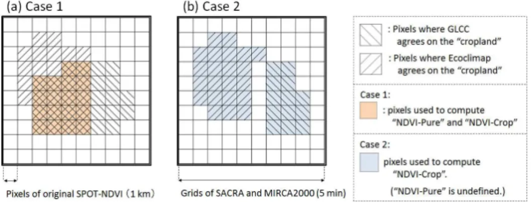
Two NDVI data sets (NDVI-Pure and NDVI-Crop; 5 arcmin resolution) are aggregated from the original SPOT-NDVI (1 km resolution) using two land cover data sets: Global Land
Figure 3. Time series of the NDVI at a double-cropping pixel in
China (116.76◦E, 32.60◦N). (a) represents the original NDVI and the NDVI with the BISE correction. (b) represents the NDVI with the BISE correction from 2004 to 2006. (c) represents the NDVI average over 2004–2006 and the normalized NDVI (nNDVI).
Figure 4. Schematic image of the aggregation of NDVI-Pure and NDVI-Crop from the 1 km resolution original NDVI. Small-sized squares
with thin lines represent pixels of the original SPOT-NDVI (1 km resolution). Large-sized squares with bold lines represent grids of SACRA and MIRCA2000 (5 arcmin resolution). Pixels with diagonal lines (from upper left to bottom right and from bottom left to upper right) show where GLCC and Ecoclimap agree on the cropland.
Figure 5. Global distribution of (a) detected cropping intensity in this study and (b) climate-based estimation of cropping intensity suitability
(i.e., maximal cropping intensity; Zabel et al., 2014). The cropping intensity of the dominant crop is illustrated in Fig. 5(b).
higher confidence grids, is used to identify the two CC pa-rameters (Sect. 2.3). The NDVI-Crop is used to produce the global CC in Sect. 2.4. The two aggregations (spatial and temporal) aim to obtain a smoother time series of the NDVI by removing the phenology of non-dominant and voluntary crops.
2.2.3 Normalization of the NDVI
Absolute peak values of the NDVI differ depending on cli-mate conditions and density of crops. Therefore, we normal-ize NDVI data to consider variety over a wide range of en-vironmental conditions at the global scale. First, we identify cropping intensity using the time series of the NDVI. We de-fine the peak of the NDVI (NDVIpk) and the date of the peak (tpk) if the time series of the NDVI satisfy Eqs. (2) and (3):
NDVI(i)≤NDVI(tpk)(i=tpk−1, tpk−2, . . ., tpk−6), (2) NDVI(i)≤NDVI(tpk)(i=tpk+1, tpk+2, . . ., tpk+4), (3) where the boundary is cyclic (i.e., NDVI0=NDVI36 and NDVI1=NDVI37) since we have 36 NDVI data per year from 10-day composite data of the SPOT-NDVI. We assume an increase/decrease in the NDVI before/after the peak of the NDVI, as shown in Eqs. (2) and (3). The cropping intensity
is equal to the number of peaks of the NDVI, up to three times per year. Second, we detect the lowest NDVI between peaks (NDVIbtm). Finally, NDVI data are normalized using the following equations:
nNDVI(t )=NDVI(t )−NDVIbas NDVIpk−NDVIbas
, (4)
NDVIbas=max(NDVIbtm,NDVIsnow), (5) where nNDVI represents the normalized NDVI. Subscripts btm, bas, and snow denote bottom, base and snow, respec-tively. The NDVIsnow is a parameter to avoid a remnant ir-regular NDVI mainly caused by snow cover reflection. The NDVIsnow is set at 0.20, which corresponds to 40 % of the snow cover over the land surface (Dye and Tucker, 2003). Figure 3c shows a schematic image of the normalization of the NDVI at the double-cropping pixel in China. As shown in Fig. 3c, the NDVIbascan be different for each peak. We do not need to avoid the negative nNDVI in this normalization process. The normalization is applied for both the NDVI-Pure and the NDVI-Crop.
inten-Table 3. Comparison of estimated cropping intensity in this study, Zabel et al. (2014), and MIRCA2000 simplified cropping intensity for
irrigated (IRC) and rain-fed (RFC) crop classes in six administrative units (six boxes A–F in Fig. 5a and b). Averaged cropping intensities over the administrative units are shown as “Cropping intensity”. “Code” and “Crop” represent the assigned code of the administrative unit in SACRA and the dominant crop in the major cultivation season in this study. The simplified cropping intensities are annual harvested area divided by maximum monthly cropped area, which are defined for both irrigated and rain-fed classes of 26 crop types.
Cropping intensity (yr−1)
Code Box in Fig. 5 Name of administrative unit Crop This study Zabel et al. (2014) MIRCA IRC MIRCA RFC 073 A Brazil Rio Grande do Sul MAZ 1.2 3.0 1.0 1.0
109 B China Henan SWH 2.2 1.0 1.0 1.0
157 C France SWH 1.3 1.0 1.0 1.0
211 D India Uttar Pradesh TWH 2.0 1.0 2.0 1.1
227 E Kenya MAZ 1.8 1.3 1.0 1.0
364 F US Mississippi SOY 0.8 2.1 1.0 1.0
TWH: temperate-wheat; SWH: snow-wheat; MAZ: maize; and SOY: soybean.
Figure 6. Time series of the NDVI for six administrative units in Table 3; Brazil Rio Grande do Sul (code 73), China Henan (code 109),
France (code 157), India Uttar Pradesh (code 211), Kenya (code 227), and US Mississippi (code 364). Black lines show time series of NDVI-Crop averaged over 2004–2006 in the administrative units (i.e., the NDVI of all grids in the administrative units). Green lines show the average of black lines (i.e., averaged over the administrative units). Red, blue, and magenta represent NDVI-Crop in 2004, 2005, and 2006, respectively, averaged over the administrative units.
sity (i.e., maximal cropping intensity) suitability for current climate conditions (1981–2010) for 16 crop types (Table 2b). Detected and estimated cropping intensities are shown in Fig. 5a and b. Since Zabel et al. (2014) estimated cropping intensities for 16 crops, we illustrate the cropping intensity of the dominant crop in the major cultivation season in SACRA. The locations of six administrative units are emphasized with boxes (A–F) in Fig. 5a and b, where our estimations are dif-ferent from those of Zabel et al. (2014).
Table 3 shows a comparison of estimated cropping inten-sity in this study and that of Zabel et al. (2014) for the six administrative units (six boxes A−F in Fig. 5a and b). For the comparison, a simplified cropping intensity for irrigated (IRC) and rain-fed (RFC) crop classes from MIRCA2000 is also described. Here, simplified cropping intensities are defined as “annual harvested area” divided by “maximum monthly cropped area”, which are defined for both irrigated and rain-fed classes of 26 crop types in MIRCA2000. The
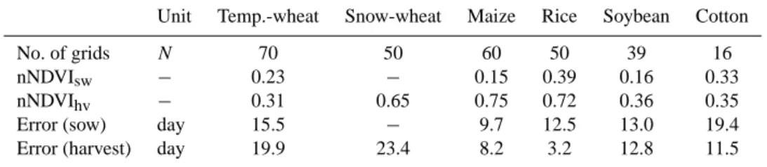
Table 4. Number of calibration grids, two calibrated crop calendar parameters (nNDVIswand nNDVIhv), and averaged errors (nNDVI) in
sowing/harvesting dates between determined crop calendar and MIRCA2000 among calibration grids of the six crop types.
Unit Temp.-wheat Snow-wheat Maize Rice Soybean Cotton No. of grids N 70 50 60 50 39 16 nNDVIsw − 0.23 − 0.15 0.39 0.16 0.33 nNDVIhv − 0.31 0.65 0.75 0.72 0.36 0.35
Error (sow) day 15.5 − 9.7 12.5 13.0 19.4 Error (harvest) day 19.9 23.4 8.2 3.2 12.8 11.5
in some grids because of uncertainty in the land cover data and insufficient spatial resolution (see Sect. 3.3 for further discussion).
In China Henan (box B), India Uttar Pradesh (box D), and Kenya (box E), the average cropping intensity in this study is larger than in Zabel et al. (2014) and MIRCA2000, with the only exception being irrigated crop in MIRCA2000 in India Uttar Pradesh. In India Uttar Pradesh, the har-vested area of irrigated crops is larger than that of rain-fed crops (cf. Table I-211 in Portmann, 2011), suggesting our estimation of cropping intensity corresponds to the ir-rigated crop. We see clear trimodal and bimodal NDVI-Crop (green lines) in China Henan and Kenya (Fig. 6b and e). Again, Fig. 5b shows the average cropping intensity for the dominant crop in the major cultivation season, according to Zabel et al. (2014). Generally, farmers do not conduct mul-tiple cropping with wheat only. Zabel et al. (2014) reported multiple-cropping intensities for other crops in two admin-istrative units. The other possibility is that overestimations of cropping intensity derive from a mixture of phenology from different crops or vegetation in France (box C). On the other hand, Zabel et al. (2014) and MIRCA2000 may under-estimate cropping intensity in Kenya, where a clear bimodal NDVI-Crop (green line) is detected in Fig. 6e. It is also possi-ble that the bimodal NDVI-Crop can be derived from mixture of phenology from different crops.
2.3 First estimation of global crop calendar
This study estimates sowing and harvesting dates (tsw and thv) using two CC parameters (nNDVIswand nNDVIhv) and a time series of nNDVI data. The sowing and harvesting dates are determined by the following:
t= tsw thv when
t≤tpkand nNDVI(t )≥nNDVIsw t≥tpkand nNDVI(t )≥nNDVIhv
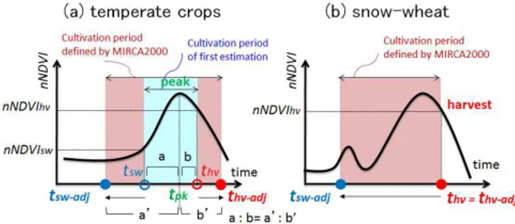
, (6) where subscripts sw and hv denote sowing and harvest, re-spectively. Figure 7a and b show schematics of identifica-tion of sowing and harvesting dates for temperate crops (temperate-wheat, rice, maize, soybean, and cotton) and snow-wheat. In the multiple cropping grids, sowing and har-vesting dates are also determined for each cropping season (except for the sowing date of snow-wheat). Our method is unsuitable for the estimation of sowing dates of snow-wheat
Figure 7. Scheme of identification of sowing and harvesting dates
in this study. Sowing and harvesting dates (tswandthv) are
identi-fied together with a vegetation index time series (black lines) and two crop calendar (CC) parameters: nNDVIswand nNDVIhv. (a)
and (b) indicate temperate crops (temperate-wheat, maize, rice, soy-bean, and cotton) and snow-wheat, respectively. The two CC param-eters are defined for the six crop types (Table 2a).
because we assume an increase in the NDVI from sowing date to peak in Eq. (6). However, the NDVI decreases if the surface is covered by snow (Fig. 7b). Therefore, in this pro-cess, we determine both sowing and harvesting dates for tem-perate crops, and only the harvesting date for snow-wheat. The two CC parameters used for the determination of sow-ing and harvest dates are defined for each crop type with the exception of the nNDVIswof snow-wheat. We calibrated the two CC parameters (nNDVIswand nNDVIhv) for each crop type as described in the following paragraph.
calibra-Figure 8. Scheme used to adjust the cultivation period of SACRA
to that of MIRCA2000.tsw(thv) andtsw−adj(thv−adj) denote
sow-ing (harvestsow-ing dates) for the first estimation and subsequent to the adjustment, respectively. For temperate crops, sowing and har-vesting dates are moved (advanced or postponed) to adjust the cultivation period to MIRCA2000. In this treatment, the ratio of
tpk−tswto thv−tpk is preserved as the ratio oftpk−tsw−adjto thv−adj−tpk. For snow-wheat, the harvesting date has not changed
(i.e., thv=thv−adj). Sowing date is determined by the cultivation
period of MIRCA2000 and the harvesting date of the first estima-tion.
tion grids between determined sowing/harvesting dates and MIRCA2000 (see Appendix A for details). Table 4 shows the number of calibration grids, the calibrated two CC pa-rameters and averaged errors in sowing/harvesting dates for six crop types.
2.4 SACRA data sets
The global sowing and harvesting dates are determined by Eq. (6) using time series of the nNDVI-Crop and two CC pa-rameters (first estimation in Fig. 1, except for the sowing date of snow-wheat). Our method detects the cultivation season using time series of the satellite-sensed NDVI. However, our algorithm carries the possibility of overestimating or under-estimating cultivation periods. The cultivation period (from sowing date to harvesting date) in our scheme is largely af-fected by the shape of the NDVI (i.e., kurtosis of the NDVI curve). Therefore, our method can result in unrealistic cul-tivation periods in some grids (e.g., less than 60 days) if NDVI-Crop does not represent the phenology of the dom-inant crops due to mixture of phenology from other crops and vegetation. Therefore, we adjust the length of the culti-vation period to be equal to MIRCA2000 to avoid the unreal-istic cultivation periods. For the temperate crops, sowing and harvesting dates are moved (advanced or postponed) to ad-just the cultivation period to MIRCA2000. In this treatment, the ratio oftpk−tsw tothv−tpk is preserved as the ratio of tpk−tsw−adjtothv−adj−tpk, (Fig. 8a), wheretsw(orthv) and tsw−adj (or thv−adj) denote sowing (or harvesting) dates for the first estimation and after the adjustment, respectively. For snow-wheat, the harvesting date is fixed (i.e.,thv=thv−adj). The sowing date is determined by the cultivation period of MIRCA2000 and the harvesting date of the first estimation
(Fig. 8b). Here, we use the cultivation period in MIRCA2000 from the 15th of the sowing month to the 15th of the harvest-ing month. For multiple-croppharvest-ing grids, the correspondharvest-ing cultivation season in MIRCA2000 (i.e., major or second cul-tivation seasons) from each cropping is determined by the following: major season second season when
Monsw(major),1st≤tpk<Monsw(second),1st Monsw(second),1st≤tpk<Monsw(major),1st
, (7)
where Monsw,1st denotes the 1st of the sowing month in MIRCA2000. Subscripts major and second denote major and second cultivation seasons, respectively. Here, we consider the cyclic boundary of the calendar. We apply the cultiva-tion period of the major cultivacultiva-tion season in grids where no dominant crop in the second cultivation season is defined. The adjusted sowing and harvesting dates are referred to as SACRA and are discussed in the next section.
3 Results and discussion
This section provides validation and discussion regarding the produced SACRA data set. However, true validation is hard to achieve in global studies. Therefore, we compare the esti-mated CC with other CC data produced using other estima-tions, either census-based or model-based.
3.1 Comparison with census-based and model-based approaches
We compare SACRA with two CC data sets: MIRCA2000 and Waha et al. (2012; hereafter W12). We selected MIRCA2000 and W12 arbitrarily as representing census-based and model-census-based CC data, respectively. Waha et al. (2012) simulated the sowing dates of major annual crops from 1900 to 2003 at a spatial resolution of 0.5◦. We use the averaged sowing dates (2000–2003) of four crops (wheat, rice, maize and soybean) from W12 for comparison. Waha et al. (2012) assigned 1 January as the sowing date, as it is as good as any other day for sowing in a favorable all-year climate. Therefore, averaged sowing dates are computed, ex-cluding grids assigning 1 January as the sowing date. Note that the sowing date of cotton was not estimated in W12. The averaged sowing date over years is computed by the follow-ing:
ηyear,sw=F (DOYyear,sw)=
DOYyear,sw
Days of the year·2π (8) DOYave,sw=F−1arg average cos ηyear,sw
+i·average sin ηyear,sw , (9)
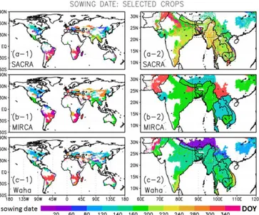
Figure 9. Sowing dates (unit: day of year) of dominant crops in
the major cultivation season for (a) SACRA, (b) MIRCA2000, and
(c) Waha et al. (2012). Left panels (a-1, b-1, and c-1) and right
panels (a-2, b-2, and c-2) show global and South Asian maps, re-spectively. Sowing dates are illustrated in grids where the dominant crop is temperate-wheat, snow-wheat, maize, rice, soybean or cot-ton. The major seasons at multiple cropping grids are determined by Eq. (7) for SACRA. Panels of SACRA contain sowing dates of the major cultivation season for both single and multiple cropping grids. Boxes in right panels represent the area where SACRA did not detect the crop calendar in some grids while MIRCA2000- and Waha et al. (2012)-defined.
subscript ave denotes average.FandF−1define functions to computeηfrom DOY and DOY fromη, respectively. Equa-tions (8) and (9) are used to compute the averaged sowing date considering the cyclic boundary of the calendar.
The spatial distributions of the sowing dates for the dom-inant crops in the major cultivation season for SACRA, MIRCA2000 and W12 are shown in Fig. 9. The sowing dates are illustrated in grids where the dominant crop of SACRA in the major cultivation season is temperate-wheat, snow-wheat, maize, rice, soybean or cotton. If multiple sowing exists in the SACRA dates for the major cultivation sea-son, we illustrate the sowing dates derived from the largest NDVIpk among the sowing dates. For MIRCA2000, we il-lustrate the 15th of the sowing month. Although three differ-ent sets of data are produced from the differdiffer-ent approaches (Earth observation-based, census-based, and model-based), they have similar spatial patterns (Fig. 9a-1, b-1, and c-1). Their sowing dates generally represent spring in their grids. Figure 9a-2, b-2, and c-2 show the sowing dates in South Asia, selected arbitrarily to highlight the higher spatial vari-ability in SACRA. Since SACRA uses high-resolution satel-lite data, it reflects a variety of sowing dates in the same ad-ministrative unit, as shown in Fig. 9a-2 (e.g., Thailand, Viet-nam, and Laos). W12 also resulted in a variety of sowing
dates for Vietnam (Fig. 9c-2) due to the estimation being based on climatic data. The detection of variability in the CC within an administrative unit is an advantage of Earth-observation-based and model-based approaches compared to census-based methods. On the other hand, SACRA carries the disadvantage of undetection of a crop calendar in grids where the NDVI-Crop is not defined (boxes in Fig. 9a-2, b-2, and c-2).
While SACRA can detect the variability of the CC within administrative units, it is difficult to demonstrate whether the variability is correct around the globe without knowledge of the local CC information. Therefore, the following subsec-tion discusses the differences in the CCs among the three products, with sowing dates. We compare the sowing dates of the three products averaged over administrative units de-fined in MIRCA2000.
3.2 Comparison of averaged CC over MIRCA2000 administrative units
To investigate the characteristics of the three approaches, we compare the averaged sowing dates over administrative units. The averaged sowing dates of the dominant crop in the major cultivation season are computed by three products (SACRA, MIRCA2000, and W12) using Eqs. (8) and (9), averaging not over years but over administrative units. We assign the 15th of the sowing month for MIRCA2000. The sowing dates of temperate- and snow-wheat in SACRA are compared with the sowing dates of “wheat” in MIRCA2000 and W12. Here, only single cropping grids are used to compute the averaged sowing date for SACRA. We suppose that NDVIbas repre-sents the condition with little vegetation in the winter (or dry) season. In the multiple cropping grids, the NDVIbasin the summer (or wet) season can be higher than other seasons due to mixture of phenology from other crops and vegeta-tion (e.g., NDVIbas in June is higher than that in December in Fig. 3c). Therefore, accuracy of CCs in multiple cropping grids may be lower than that in single cropping grids.
The differences in the sowing dates of the dominant crop are shown in Fig. 10. The administrative units are illustrated if their dominant crop in the major cultivation season is temperate-wheat, snow-wheat, maize, rice, soybean or cot-ton. The difference for each specific crop type is shown in Fig. A3. The difference between the two data sets is less than 2 months (< 62 days; yellow- or green-colored units) in most of the administrative units in Fig. 10a and b. Figure A3 shows that wheat contains the largest number of units, with a large difference in sowing dates (> 93 days; red- or blue-colored units). We observe a later signalling trend in sowing dates in SACRA than in W12 (Fig. 10b; green- or blue-colored units). The direction of the later signalling trend is dominant in wheat, maize, rice and soybean (Fig. a2, b2, A3-c2, and A3-d2).
Figure 10. Differences in sowing dates of the dominant crop in the major cultivation season (a: SACRA–MIRCA2000; b: SACRA–Waha
et al., 2012). The administrative units are illustrated if their dominant crop in the major cultivation season is temperate-wheat, snow-wheat, maize, rice, soybean or cotton. The differences for each specific crop type are shown in Fig. A3. Only single cropping grids are used to compute the averaged sowing date for SACRA.
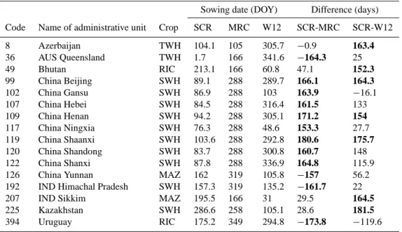
Table 5. Administrative units with large absolute differences in sowing date (> 150 days) between SACRA and MIRCA2000 or SACRA and
Waha et al. (2012). SCR, MRC, and W12 in the table represent SACRA, MIRCA2000, and Waha et al. (2012), respectively. “Code” and “Crop” represent the assigned code of the administrative unit in SACRA and the dominant crop in the major cultivation season in this study. Bold numbers denote large absolute differences in sowing date between SACRA and the other data sets. The table compares sowing dates averaged over the administrative units. Only single cropping grids are used to compute the averaged sowing date for SACRA.
Sowing date (DOY) Difference (days) Code Name of administrative unit Crop SCR MRC W12 SCR-MRC SCR-W12 8 Azerbaijan TWH 104.1 105 305.7 −0.9 163.4
36 AUS Queensland TWH 1.7 166 341.6 −164.3 25 49 Bhutan RIC 213.1 166 60.8 47.1 152.3
99 China Beijing SWH 89.1 288 289.7 166.1 164.3
102 China Gansu SWH 86.9 288 103 163.9 −16.1 107 China Hebei SWH 84.5 288 316.4 161.5 133 109 China Henan SWH 94.2 288 305.1 171.2 154
117 China Ningxia SWH 76.3 288 48.6 153.3 27.7 119 China Shaanxi SWH 103.6 288 292.8 180.6 175.7
120 China Shandong SWH 83.7 288 300.8 160.7 148 122 China Shanxi SWH 87.8 288 336.9 164.8 115.9 126 China Yunnan MAZ 162 319 105.8 −157 56.2 192 IND Himachal Pradesh SWH 157.3 319 135.2 −161.7 22 207 IND Sikkim MAZ 195.5 166 31 29.5 164.5
225 Kazakhstan SWH 286.6 258 105.1 28.6 181.5
394 Uruguay RIC 175.2 349 294.8 −173.8 −119.6
TWH: temperate-wheat; SWH: snow-wheat; MAZ: maize; RIC: rice; COT: cotton; AUS: Australia; IND: India.
disagreement (more than 150 days) between SACRA and MIRCA2000 or SACRA and W12. We present the cultiva-tion seasons (from sowing to harvesting dates) in 16 admin-istrative units in Fig. A4 to understand the discrepancies in the CCs of the three products. To interpret the disagreements in Table 5 and Fig. A4, we use Fig. 11, which shows the time series of the NDVI-Crop, average NDVI-Crop, average NDVI-Forest, and average temperature data. Here, average means the average over administrative units. NDVI-Forest is produced by following NDVI-Crop production, but with for-est pixels using GLCC and Ecoclimap land cover data. That
is, NDVI-Forest is aggregated by averaging the pixels where the GLCC or Ecoclimap agree on forest.
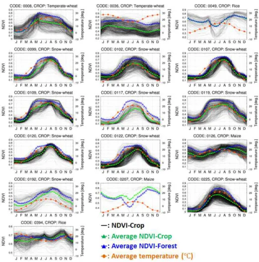
Figure 11. Time series of NDVI-Crop (black lines), average NDVI-Crop (green lines), average NDVI-Forest (blue lines), and average
temperature (orange lines;◦C) in the 16 administrative units in Table 5; Azerbaijan (code 8), Australia Queensland (code 36), Bhutan (code
49), China Beijing (code 99), China Gansu (code 102), China Hebei (code 107), China Henan (code 109), China Ningxia (code 117), China Shaanxi (code 119), China Shandong (code 120), China Shanxi (code 122), China Yunnan (code 126), India Himachal Pradesh (code 192), India Sikkim (code 207), Kazakhstan (code 225), and Uruguay (code 394). The average denotes the average over the administrative units.
in the spring and matures in late summer, but can be sown in the fall in countries that experience mild winters, such as in South Asia, North Africa, the Middle East, and at lower latitudes.
In Azerbaijan (code 8) and Kazakhstan (code 225), large differences (> 150 days) are observed between SACRA and W12, while the differences between SACRA and MIRCA2000 are < 50 days. In Australia Queensland (code 36), China Gansu (code 102), China Ningxia (code 117), and India Himachal Pradesh (code 192), a large difference is observed between SACRA and MIRCA2000. In the above six administrative units, the assumed wheat type may be in-correctly identified in MIRCA2000 and W12. On the other hand, SACRA’s sowing dates differ from both MIRCA2000 and W12 for Beijing (code 99), Hebei (code 107), Henan (code 109), Shaanxi (code 119), Shandong (code 120), and Shanxi (code 122) in China. In these six administrative units, SACRA has possibly detected incorrect signals of the NDVI (e.g., signals of forest or other crops). As shown in Fig. A3,
wheat is related to the largest number of units with disagree-ments in sowing dates. Disagreedisagree-ments in sowing dates are also observed between MIRCA2000 and W12. The identifi-cation of wheat type (sowing in spring or fall) may be a major source of error in global CC estimations.
In Bhutan (code 49), India Sikkim (code 207), and Uruguay (code 394), clear unimodal NDVI-Crops are not ob-served in Fig. 11. The accuracy of SACRA is affected by the accuracy of the land cover data sets. It is known that the 1 km land cover data sets contain uncertainties (Herold et al., 2008; Nakaegawa, 2012). For example, forests may be classified as croplands in the 1 km land cover data sets. Also, NDVI and land cover data sets at 1 km resolution may be insufficient to detect the phenology of the dominant crop in the administra-tive units.
a mixed phenology of non-dominant and voluntary crops. Our approach is unable to consider a mixture of phenology. This may explain the disagreement between SACRA’s sow-ing dates and those of other products.
A major discrepancy in crop calendars between SACRA and other products can be due to the selection of one dom-inant crop in each administrative unit. It is possible that SACRA detects the CC of similar maximal harvested area or another sub-crop in MIRCA2000 (e.g., for irrigated wheat in India Uttar Pradesh with two identical areas with different cropping periods; cf. Table I-211 of Appendix I in Portmann, 2011). The disadvantages of our approach may be reduced with future improvements based on finer satellite sensors to avoid mixture of phenology from other crops and vegetation, and crop-type classification studies to consider several dom-inant crops in each grid.
Taking into account the extreme disagreement between SACRA and MIRCA2000 or W12 in some regions (Table 5 and Fig. 10), it becomes important to determine which CC is more reliable. However, it is difficult to decide which data set is more accurate in global studies. For example, the identifi-cation of the wheat type (sowing in spring or fall) is difficult, as shown in disagreements among the three products in 12 administrative units (Table 5). Also, it is possible that both are correct, e.g., if they referred to different time periods. MIRCA2000 possibly used the conditions of nearby admin-istrative units because of a lack of more detailed reference information. Therefore, it is difficult to determine the abso-lute accuracy of the products through comparison. However, combined application of several products is useful for tak-ing the uncertainty of the CC into account. Since SACRA, MIRCA and W12 detect the CC from different approaches, a comparison of their results is useful for cross-validation. 3.3 Advantages and disadvantages of SACRA
This subsection discusses the advantages and disadvantages of SACRA compared to two other approaches: census-based and model-based methods. Additionally, this subsection also discusses possible improvements of SACRA. Table 6 sum-marizes the advantages and disadvantages of the census-based methods, model-census-based methods, and SACRA.
An advantage of SACRA is its fine spatial resolution com-pared to the other two data sets. Therefore, different CCs in the same administrative unit are considered in SACRA (Fig. 9a-2). The model-based method can also result in a va-riety of CCs. However, it is difficult to demonstrate that the variability is correct around the globe without knowledge of local CC information.
The spatial resolution of SACRA is equal to the maximum resolution of the satellite-sensed NDVI and the crop clas-sification map. At present, the NDVI from the MODerate-resolution Imaging Spectroradiometer (MODIS) is available at a spatial resolution of 250 m (e.g., Zhang et al., 2006). However, present studies provide global crop classification
maps at a spatial resolution of 5 arcmin (e.g., Monfreda et al., 2008; Portmann et al., 2010). Present land cover data sets, such as GLCC and Ecoclimap, only contain a small num-ber of coarse agricultural classes. At the regional scale, many studies have been performed to classify crops using satellite-sensed data (e.g., Mingwei et al., 2008; Wardlow and Eg-bert, 2008; Wardlow et al., 2007). In this study, we use the crop classification map from MIRCA2000 at a spatial reso-lution of 5 arcmin. SACRA can be recalculated with higher-resolution remote sensing data (e.g., from future Sentinel-2 data; Drusch et al., Sentinel-201Sentinel-2) if higher-resolution land cover maps become available. The higher-resolution CC products can contribute to hydrological/agricultural studies that aim to conduct simulations at a spatial resolution of 1 km (e.g., Wood et al., 2011; Kotsuki et al., 2015).
A second advantage of SACRA is its easy detection of cul-tivation using time series of the NDVI. Because agriculture is controlled by human decisions, it is difficult to estimate from the census-based and model-based methods whether or not farmers actually perform cultivation. Additionally, agricul-ture is affected by disasters, such as droughts, inundations, heat waves, and cool summer damages. The satellite-sensed NDVI can be used to detect whether the managed land is cur-rently being cultivated or is temporarily in disuse. It is also possible to identify cropping intensity with time series of the NDVI (Fig. 5).
However, SACRA has the disadvantage that it is inappli-cable to future simulations such as impact assessments of cli-mate change because SACRA is produced using past obser-vational data. Future changes in agricultural water demand and biomass production are major issues in assessment stud-ies of climate change (Hanjra and Qureshi, 2010). An advan-tage of SACRA compared to MIRCA2000 is that SACRA provides not only sowing/harvesting dates but also the peak date from the time series of the NDVI. The peak date can be used to calibrate the parameters of crop growth models that simulate the growing stage during cultivation (e.g., Horie 1987). SACRA can contribute to future assessment studies indirectly by being utilized to calibrate their model parame-ters.
adjust-Table 6. Advantages and disadvantages of three types of global crop calendars: census-based, model-based, and Earth observation-based.
Census-based Model-based Earth observation-based Main inputs Census data Forcing data Satellite-sensed NDVI Resolution Country/state scale Equal to forcing data 5 arcmin
Different CC in same admin. unit Impossible Possible Possible Detection of cultivation Hard Hard Easy Mixture of several crops in a grid Possible Possible Impossible Application to future simulations Impossible Possible Impossible
ment. Also, utilization of snow cover products from satellite (e.g., the MODIS snow cover product; Hall et al., 2002) or land surface data assimilation (e.g., the global land data as-similation system; Rodell et al., 2004) would help to adjust the sowing date of snow-wheat appropriately.
Our method has the disadvantage that the mixture of sev-eral crops in a grid is not considered. Therefore, we assume that the NDVI-Crop represents the phenology of the domi-nant crop at each grid. Because of this assumption, our ap-proach contains the following disadvantages: (1) the census-based and model-census-based approaches can contain CCs for more than one crop for every unit (e.g., MIRCA2000 and W12), while SACRA only contains the CC for the dominant crop in a given unit; (2) census-based data can deliver a CC for either irrigated or rain-fed crops, while SACRA cannot sepa-rate them. In fact, CCs for irrigated and rain-fed cropland can be different; and (3) our approach cannot consider the mix-ture of phenology from several crops and voluntary crops. It should also be noted that the length of the cultivation period in SACRA is adjusted to MIRCA2000 to avoid the unrealis-tic cultivation periods. A major discrepancy in crop calendars between SACRA and other products can be due to the selec-tion of one dominant crop in each administrative unit. The disadvantages of our approach would be reduced with future improvements based on finer satellite sensors and crop-type classification studies to consider several dominant crops in each administrative unit.
The idea behind CC estimation in SACRA is very simple, and therefore easily applicable to the global cropland and ad-ditional satellite observations. Due to data scarcity, we resort to averaged data from three consecutive years (2004–2006). The data product generated from this study therefore is of limited use for the direct parameterization of global growth models. However, taking into account the current develop-ment in Earth observation (e.g., the developdevelop-ment of the Euro-pean Space Agency’s Sentinel series), data scarcity will soon be less of an issue. The proposed method represents a simple and thus easily applied approach that can potentially make use of large amounts of temporally, highly resolved, global, optical, Earth observation data, and may provide interesting input parameters for global land surface models. For exam-ple, the estimation of an annual crop calendar is a major part of our scope.
Finally, the accuracy of SACRA depends on the accuracy of the NDVI and land cover data sets. The wavelengths re-quired for the calculation of the NDVI are relatively easy to measure from satellite sensors. Therefore, the accuracy of the NDVI largely depends on the temporal resolution of adequate observations (e.g., the revisiting time of the applied systems and weather at satellite observation, such as cloud cover). Us-age of several satellite sensors (e.g., MODIS) would help to reduce the uncertainty of the NDVI. With respect to the accu-racy of land cover data, we combine two land cover data sets to reduce the uncertainty of the land cover data. The land cover data sets, however, contain uncertainties (Herold et al., 2008; Nakaegawa, 2012). The land cover data sets could be improved by developing new algorithms, increasing the amount of supervised data, and utilizing multi-spectrum in-formation. Further improvements of the land cover data sets would contribute to improvement of SACRA.
4 Summary
This study aimed at producing a new crop calendar, SACRA, using a satellite-sensed NDVI. This paper describes the methods to produce SACRA from the following four data sets: time series of the NDVI, land cover data sets, reanal-ysis temperature, and census monthly agricultural data. The resulting SACRA data set included three products at a spatial resolution of 5 arcmin: (1) the spatial distribution of the dom-inant crop in major and second cultivation seasons; (2) time series of the NDVI of the cropland; and (3) sowing, peak, and harvesting dates of the dominant crop. The advantages and disadvantages of SACRA compared to other global crop calendars are summarized as follows.
SACRA can potentially be used to calibrate the parameters of crop growth models. An advantage of SACRA compared to census-based crop calendars is that SACRA provides not only sowing/harvesting dates, but also a peak date from the time series of NDVI data.
Appendix A: Calibration of crop calendar parameters This appendix describes the scheme used to calibrate two crop calendar parameters (nNDVIsw and nNDVIhv) from NDVI-Pure in Sect. 2.3. Once two parameters are given, the sowing/harvesting dates are uniquely determined with Eq. (6). We calibrated the two CC parameters so as to min-imize the error between the determined and MIRCA2000 sowing (harvesting) dates among calibration grids. Here, the error for the sowing (harvesting) date is calculated by
ERRsw(hv)=0 if Monsw(hv),1st≤tsw(hv)≤Monsw(hv),End else ERRsw(hv)=min
tsw,(hv)−Monsw(hv),1st ,
tsw,(hv)−Monsw(hv),End
, (A1)
Figure A1. Average error of sowing/harvesting dates (blue/orange lines; unit days) among calibration grids for six crops (a: temperate-wheat; b: snow-wheat; c: maize; d: rice; e: soybean; and f: cotton). Dots in the figures represent minimized errors and nNDVIswor nNDVIhv(i.e.,
the two calibrated parameters in Table 4).
Figure A2. Global distribution of calibration grids for the six crops. The calibration grids are illustrated larger than the real grid size
Figure A3. Same as Fig. 9 but for five specific crops (wheat, maize, rice, soybean, and cotton). The sowing date of cotton was not estimated
Figure A4. Cultivation seasons (from sowing to harvesting dates) in 16 administrative units in Table 5. Magenta, blue, and green denote
Appendix B: Comparison of sowing dates
Acknowledgements. K. Waha kindly provided the valuable data on
sowing dates. We gratefully acknowledge two anonymous referees for their invaluable and constructive suggestions. This study was supported in part by the Japan Society for the Promotion of Science (JSPS) KAKENHI grants 12J03816, 22246066, and 15K18128, and the SOUSEI program of the Ministry of Education, Culture, Sports, Science, and Technology.
Edited by: A. Loew
References
Döll, P. and Siebert, S.: Global modeling of irrigation water requirements, Water Resour. Res., 38, 1037, doi:10.1029/2001WR000355, 2002.
Drusch, M., Del Bello, U., Carlier, S., Colin, O., Fernandez, V., Gascon, F., Hoerschb, B., Isolaa, C., Laberintia, P., Marti-morta, P., Meygretc, A., Spotoa, F., Sya, O., Marchesed, F., and Bargellini, P.: Sentinel-2: ESA’s optical high-resolution mission for GMES operational services, Remote Sens. Environ., 120, 25– 36, doi:10.1016/j.rse.2011.11.026, 2012.
Dye, D. G. and Tucker, C. J.: Seasonality and trends of snow cover, vegetation index, and temperature in northern Eurasia, Geophys. Res. Lett., 30, 1405, doi:10.1029/2002GL016384, 2003. Food and Agriculture Organization of the United Nations:
Bread wheat, FAO Plant Production and Protection Series 30, Rome, Italy, available at: http://www.fao.org/docrep/006/ y4011e/y4011e04.htm, last access: 2 November 2015.
Faroux, A., Kaptuè Tchuentè, A. T., Roujean, J.-L., Masson, V., Maritin, E., and Le Moigne, P.: ECOCLIMAP-II/Europe: a twofold database of ecosystems and surface parameters at 1 km resolution based on satellite information for use in land surface, meteorological and climate models. Geosci. Model Dev., 6, 563– 582, doi:10.5194/gmd-6-563-2013, 2013.
Fischer, G., Velthuizen, H., and Nachtergaele, F.: Global Agro-Ecological Zones Assessment: Methodology and Results. In-terim report. Luxemburg, Austria: International Institute for Sys-tems Analysis (IIASA), and Rome: FAO, 2000.
Hall, D. K., Riggs, G. A., Salomonson, V. V., DiGirolamo, N. E., and Bayr, K. J.: MODIS snow-cover products, Remote Sens. Environ., 83, 181–194, doi:10.1016/S0034-4257(02)00095-0, 2002.
Hanasaki, N., Kanae, S., Oki, T., Masuda, K., Motoya, K., Shi-rakawa, N., Shen, Y., and Tanaka, K.: An integrated model for the assessment of global water resources – Part 2: Applica-tions and assessments, Hydrol. Earth Syst. Sci., 12, 1027–1037, doi:10.5194/hess-12-1027-2008, 2008.
Hanjra, M. A. and Qureshi, M. E.: Global water crisis and future food security in an era of climate change, Food Policy, 35, 365– 377, doi:10.1016/j.foodpol.2010.05.006, 2010.
Herold, M., Mayaux, P., Woodcock, C. E., Baccini, A., and Schmullius, C.: Some challenges in global land cover map-ping?: An assessment of agreement and accuracy in exist-ing 1 km datasets, Remote Sens. Environ., 112, 2538–2556, doi:10.1016/j.rse.2007.11.013, 2008.
Hirabayashi, Y., Kanae, S., Motoya, K., Masuda, K., and Petra, D.: A 59-year (1948–2006) global near-surface meteorological data set for land surface models – Part I: Development of daily forcing
and assessment of precipitation intensity, Hydrol. Res. Lett., 2, 36–40, doi:10.3178/HRL.2.36, 2008.
Horie, T.: A model for evaluating climate productivity and water balance of irrigated rice and its application to Southeast Asia, Southeast Asian Studies, 25, 62–74, 1987.
Kotsuki, S., Takenaka, H., Tanaka, K., Higuchi, A., and Miyoshi, T.: 1 km-resolution land surface analysis over Japan: Impact of satellite-derived solar radiation, Hydrol. Res. Lett., 9, 14–19, doi:10.3178/hrl.9.14, 2015.
Krysanova, V., Wechsung, F., Arnold, J., Srinivasan, R., and Williams, J.: SWIM (Soil and Water Integrated Model) User Manual, Potsdam Institutefor Climate Impact Research, Pots-dam, Germany, 2000.
Loveland, T. R., Reed, B. C., Brown, J. F., Ohlen, D. O., Zhu, Z., Yang, L., and Merchant, J. W.: Development of a global land cover characteristics database and IGBP DISCover from 1 km AVHRR data, Int. J. Remote Sens., 21, 1303–1330, doi:10.1080/014311600210191, 2000.
Maisongrande, P., Duchemin, B., and Dedieu, G.: VEGETA-TION/SPOT: an operational mission for the Earth monitoring; presentation of new standard products, Int. J. Remote Sens., 25, 9–14, doi:10.1080/0143116031000115265, 2004.
Mingwei, Z., Qingbo, Z., Zhongxin, C., Jia, L., Yong, Z., and Chongfa, C.: Crop discrimination in Northern China with dou-ble cropping systems using Fourier analysis of time-series MODIS data, Int. J. Appl. Earth Obs. Geoinf., 10, 476–485, doi:10.1016/j.jag.2007.11.002, 2008.
Monfreda, C., Ramankutty, N., and Foley, J.: Farming the planet: 2. Geographic distribution of crop areas, yields, physiological types, and net primary production in the year 2000, Global Bio-geochem. Cy., 22, 1–19, doi:10.1029/2007GB002947, 2008. Nakaegawa, T.: Comparison of Water-Related Land Cover Types
in Six 1 km Global Land Cover Datasets, J. Hydrometeorol., 13, 649–664, doi:10.1175/JHM-D-10-05036.1, 2012.
Pokhrel, Y., Hanasaki, N., Koirala, S., Cho, J., Yeh, P., Kim, H., Kanae, S., and Oki, T.: Incorporating Anthropogenic Water Reg-ulation Modules into a Land Surface Model, J. Hydrometeorol., 13, 255–269, doi:10.1175/JHM-D-11-013.1, 2012.
Portmann, F.: Global estimation of monthly irrigated and rainfed crop areas on a 5 arcminute grid, Frankfurt Hydrology Paper 09, 2011.
Portmann, F., Siebert, S., and Döll, P.: MIRCA2000 – Global monthly irrigated and rainfed crop areas around the year 2000: A new high resolution data set for agricultural and hydrological, Global Biogeochem. Cy., 24, 1–24, doi:10.1029/2008GB003435, 2010.
Pettorelli, N., Vik, J. O., Mysterud, A., Gaillard, J. M., Tucker, C. J., and Stenseth, N. C.: Using the satellite-derived NDVI to as-sess ecological responses to environmental change, Trends Ecol. Evol., 20, 503–510, doi:10.1016/j.tree.2005.05.011, 2005. Rockström, J., Falkenmark, M., Karlberg, L., Hoff, H., Rost,
S., and Gerten, D.: Future water availability for global food production: The potential of green water for increasing re-silience to global change, Water Resour. Res., 45, W00A12, doi:10.1029/2007WR006767, 2009.
D.: The global land data assimilation system, Bull. Amer. Me-teor. Soc., 85, 381–394, doi:10.1175/BAMS-85-3-381, 2004. Rost, S., Gerten, D., Bondeau, A., Lucht, W., Rohwer, J., and
Schaphoff, S.: Agricultural green and blue water consumption and its influence on the global water system, Water Resour. Res., 44, W09405, doi:10.1029/2007WR006331, 2008.
Sacks, W. J., Deryng, D., Foley, J. A., and Ramankutty, N.: Crop planting dates: an analysis of global patterns, Global Ecol. Biogeogr., 19, 607–620, doi:10.1111/j.1466-8238.2010.00551.x, 2010.
Sakamoto, T., Yokozawa, M., Toritani, H., Shibayama, M., Ishit-suka, N., and Ohno, H.: A crop phenology detection method us-ing time-series MODIS data, Remote Sens. Environ., 96, 366– 374, doi:10.1016/j.rse.2005.03.008, 2005.
Sakamoto, T., Wardlow, B. D., Gitelson, A., Verma, S. B., Suyker, A. E., and Arkebauer, T. J.: A Two-Step Filtering ap-proach for detecting maize and soybean phenology with time-series MODIS data, Remote Sens. Environ., 114, 2146–2159, doi:10.1016/j.rse.2010.04.019, 2010.
Siebert, S. and Döll, P.: Quantifying blue and green virtual wa-ter contents in global crop production as well as potential pro-duction losses without irrigation, J. Hydrol., 384, 198–217, doi:10.1016/j.jhydrol.2009.07.03, 2010.
Stehfest, E., Heistermann, M., Priess, J. A., Ojima, D. S., and Alcamo, J.: Simulation of global crop production with the ecosystem model DayCent, Ecol. Model., 209, 203–219, doi:10.1016/j.ecolmodel.2007.06.028, 2007.
Tan, G. and Shibasaki, R.: Global estimation of crop produc-tivity and the impacts of global warming by GIS and EPIC integration, Ecol. Model., 168, 357–370, doi:10.1016/S0304-3800(03)00146-7, 2003.
Viovy, N., Arino, O., and Belward, A. S.: The Best In-dex Slope Extraction (BISE): A method for reducing noise in NDVI time-series, Int. J. Remote Sens., 13, 1585–1590, doi:10.1080/01431169208904212, 1992.
Waha, K., Van Bussel, L. G. J., Müller, C., and Bondeau, A.: Climate-driven simulation of global crop sowing dates, Global Ecol. Biogeogr., 21, 247–259, doi:10.1111/j.1466-8238.2011.00678.x, 2012.
Wardlow, B., Egbert, S., and Kastens, J.: Analysis of time-series MODIS 250 m vegetation index data for crop classification in the U.S. Central Great Plains, Remote Sens. Environ., 108, 290– 310, doi:10.1016/j.rse.2006.11.021, 2007.
Wood, E., Roundy, J., Troy, T., van Beek, L. P. H., Bierkens, M., Blyth, E., De Roo, A., Döll, P., Ek, M., Famiglietti, J., Gochis, D., van de Giesen, N., Houser, P., Jaffé, P., Kollet, S., Lehner, B., Lettenmaier, D., Peters-Lidard, C., Sivapalan, M., Sheffield, J., Wade, A., and Whitehead, P.: Hyperresolu-tion global land surface modeling: Meeting a grand challenge for monitoring Earth’s terrestrial water, Water Resour. Res., 47, W05301, doi:10.1029/2010WR010090, 2011.
Yorozu, K., Tanaka, K., and Ikebuchi, S.: Creating a global 1-degree dataset of crop type and cropping calendar through timeseries analysis of NDVI for GSWP simulation considering irrigation effect, Proc. of 85th AMS Annual Meeting, J6.8, 2005. Zabel, F., Putzenlechner, B., and Mauser, W.: Global Agricultural