❊♥s❛✐♦s ❊❝♦♥ô♠✐❝♦s
❊s❝♦❧❛ ❞❡
Pós✲●r❛❞✉❛çã♦
❡♠ ❊❝♦♥♦♠✐❛
❞❛ ❋✉♥❞❛çã♦
●❡t✉❧✐♦ ❱❛r❣❛s
◆◦ ✹✽✾ ■❙❙◆ ✵✶✵✹✲✽✾✶✵
❈♦♥✈❡① ❈♦♠❜✐♥❛t✐♦♥s ♦❢ ▲♦♥❣ ▼❡♠♦r② ❊st✐✲
♠❛t❡s ❢r♦♠ ❉✐✛❡r❡♥t ❙❛♠♣❧✐♥❣ ❘❛t❡s
▲❡♦♥❛r❞♦ ❘♦❝❤❛ ❙♦✉③❛✱ ❏❡r❡♠② ❙♠✐t❤✱ ❘❡✐♥❛❧❞♦ ❈❛str♦ ❞❡ ❙♦✉③❛
❏✉❧❤♦ ❞❡ ✷✵✵✸
❖s ❛rt✐❣♦s ♣✉❜❧✐❝❛❞♦s sã♦ ❞❡ ✐♥t❡✐r❛ r❡s♣♦♥s❛❜✐❧✐❞❛❞❡ ❞❡ s❡✉s ❛✉t♦r❡s✳ ❆s
♦♣✐♥✐õ❡s ♥❡❧❡s ❡♠✐t✐❞❛s ♥ã♦ ❡①♣r✐♠❡♠✱ ♥❡❝❡ss❛r✐❛♠❡♥t❡✱ ♦ ♣♦♥t♦ ❞❡ ✈✐st❛ ❞❛
❋✉♥❞❛çã♦ ●❡t✉❧✐♦ ❱❛r❣❛s✳
❊❙❈❖▲❆ ❉❊ PÓ❙✲●❘❆❉❯❆➬➹❖ ❊▼ ❊❈❖◆❖▼■❆ ❉✐r❡t♦r ●❡r❛❧✿ ❘❡♥❛t♦ ❋r❛❣❡❧❧✐ ❈❛r❞♦s♦
❉✐r❡t♦r ❞❡ ❊♥s✐♥♦✿ ▲✉✐s ❍❡♥r✐q✉❡ ❇❡rt♦❧✐♥♦ ❇r❛✐❞♦ ❉✐r❡t♦r ❞❡ P❡sq✉✐s❛✿ ❏♦ã♦ ❱✐❝t♦r ■ss❧❡r
❉✐r❡t♦r ❞❡ P✉❜❧✐❝❛çõ❡s ❈✐❡♥tí✜❝❛s✿ ❘✐❝❛r❞♦ ❞❡ ❖❧✐✈❡✐r❛ ❈❛✈❛❧❝❛♥t✐
❘♦❝❤❛ ❙♦✉③❛✱ ▲❡♦♥❛r❞♦
❈♦♥✈❡① ❈♦♠❜✐♥❛t✐♦♥s ♦❢ ▲♦♥❣ ▼❡♠♦r② ❊st✐♠❛t❡s ❢r♦♠ ❉✐❢❢❡r❡♥t ❙❛♠♣❧✐♥❣ ❘❛t❡s✴ ▲❡♦♥❛r❞♦ ❘♦❝❤❛ ❙♦✉③❛✱ ❏❡r❡♠② ❙♠✐t❤✱ ❘❡✐♥❛❧❞♦ ❈❛str♦ ❞❡ ❙♦✉③❛ ✕ ❘✐♦ ❞❡ ❏❛♥❡✐r♦ ✿ ❋●❱✱❊P●❊✱ ✷✵✶✵
✭❊♥s❛✐♦s ❊❝♦♥ô♠✐❝♦s❀ ✹✽✾✮
■♥❝❧✉✐ ❜✐❜❧✐♦❣r❛❢✐❛✳
Convex Combinations of Long Memory Estimates from Different Sampling
Rates
Leonardo R. Souza∗ Graduate School of Economics
Fundação Getúlio Vargas
Jeremy Smith Department of Economics
University of Warwick
Reinaldo C. Souza
Electrical Engineering Department Catholic University, Rio de Janeiro
Abstract: Convex combinations of long memory estimates using the same data observed at
different sampling rates can decrease the standard deviation of the estimates, at the cost of inducing a slight bias. The convex combination of such estimates requires a preliminary correction for the bias observed at lower sampling rates, reported by Souza and Smith (2002). Through Monte Carlo simulations, we investigate the bias and the standard deviation of the combined estimates, as well as the root mean squared error (RMSE), which takes both into account. While comparing the results of standard methods and their combined versions, the latter achieve lower RMSE, for the two semi-parametric estimators under study (by about 30% on average for ARFIMA(0,d,0) series).
Keywords: Convex Combination, Long Memory, Sampling Rate. JEL Codes: C13, C14, C63
∗
1 Introduction
Asymptotic self-similarity in long memory time series ensures that the memory
parameter is constant even when changing the sampling rate. Tschernig (1995), Chambers
(1998) and Souza (2003a,b) provide results on the issue. So, a convex combination of estimates
from different sampling rates can reduce the estimation variance if the bias of the estimates from
lower sampling rates is small and the correlation between the different estimates is not high. At a
first glance this is likely to occur at least for values of d close to zero. However, Souza and Smith
(2002) show that decreasing the sampling rate induces a substantial bias in some estimators (all
that were under study) due to the aliasing effect1. To overcome such a problem a bias correction
can be applied to the estimates obtained from lower sampling rates.
In this paper, we implement a procedure for combining convexly the estimates from
different sampling rates taken from the same data. This procedure is a purely artificial construct
to take advantage from asymptotic self-similarity, and to our knowledge no other
computationally intensive method for enhancing the long memory estimation upon an existing
estimator has been proposed so far. It is intended for small samples, where the root mean square
error of some long memory estimators is high, even though most of them have been proved
consistent. Correction for the bias in the memory parameter is applied to estimates from
decreased sampling rates using the heuristic formula proposed by Souza and Smith (2002). The
convex combination of the long memory estimates can decrease the standard deviation (and the
root mean squared error – RMSE) by up to 50% in some cases, however a slight bias remains.
The RMSE is reduced by about 30% on average if the process is an ARFIMA(0,d,0).
This paper is organised as follows. Section 2 briefly introduces long memory and the
effect of changing the sampling rate on it. Section 3 explains how the convex combination is
carried out and shows its results. Section 4 offers some concluding remarks.
1
2 Long memory and the sampling rate 2.1 Long memory
Long memory models are receiving more attention in the econometrics literature these
days, as many instances of apparently stationary time series with long-range dependence arise.
Among alternative definitions of long memory in stationary time series available in the literature,
we work with the following two.
The first definition refers to the asymptotic behaviour of the autocorrelations. Let Xt be a
stationary process and let ρ(k) be the k-th order serial correlation of the series Xt. If there exists a
real number d ∈ (0, 0.5) and a positive function c kρ( ) slowly varying as k tends to infinity such
that
∞ →
− ask
) ( ~ )
(k cρ k k2d 1
ρ (1)
then Xt is said to have long memory or long range dependence. When d ∈ (-0.5, 0) and c kρ( ) is
no longer positive, the process Xt is said to be “antipersistent” (Mandelbrot, 1977, p.232).
The second definition considers the spectrum behaviour close to the zero frequency, as
follows. If there exists a positive function cf(λ), λ∈(−π,π], which varies slowly as the frequency λ tends to zero, such that d ∈ (0, 0.5) and
0 as )
( ~ )
(λ cf λ λ−2d λ →
f , (1.A)
where f(λ) is the spectral density function of the stationary process Xt, then Xt is a stationary
process with long memory with (long-)memory parameter d. The behaviours defined by (1) and
(1.A) are not equivalent, but arise together with the same parameter d in a number of long
memory models, such as in the ARFIMA class of models, which is defined below, for a subset of
the parametric space.
Xt is said to follow an autoregressive integrated moving average model (ARIMA) if
Φ( )(B B X)d Θ( )B
t t
where εt is a mean zero constant variance white noise process, B is the backward shift operator,
such that BXt = Xt-1, and Φ(B) = 1-φ1B-…-φpBp and Θ(B)=1+θ1B+…+θqBq are the
autoregressive and moving average polynomials, respectively. ARIMA models allowing for a
non-integer value of the parameter d are called ARFIMA, and it can be shown (Granger and
Joyeux, 1980, Hosking, 1981) that they display long memory dependence according to (1) and
(1.A) while are still stationary when d ∈ (0, 0.5) and the roots of Φ(B) are outside the unit circle. The fractional difference can be more easily understood by expanding the polynomial (1-B)d in a
binomial series, yielding an infinite AR polynomial:
( ) ( )
( ) ( ) 1
1
0
− = − + −
= ∞
B j d B j d
d
j
j
Γ
Γ Γ (3)
where Γ(.) is the gamma function.
2.2 Estimators
In this paper we consider two semiparametric estimators, the one proposed by Geweke
and Porter-Hudak (1983), henceforth GPH, and its smoothed version, SMGPH, proposed by
Hassler (1993). Choosing semiparametric long memory estimators (instead of parametric ones)
implies that not all the spectrum will be considered, but only a band of it, discarding short
memory components are known to bias the estimation. On the other hand, using a parametric
estimator would require a prior specification for the model. The use of only a band of
frequencies poses the question as to which bandwidth to choose, and there is a trade-off between
bias and standard deviation implied by such choice. The wider the bandwidth, the more biased
the estimator will be, but, on the other hand, the lower standard deviation it will achieve. It is
well known that a positive autoregressive component bias upward and a negative moving
average2 component bias downward long memory estimation (Smith, Taylor and Yadav, 1997,
Souza and Smith, 2002), the bias increasing with the parameter value. On the other hand,
2
negative autoregressive or positive moving average components do not bias considerably the
estimation.
The GPH estimator, proposed by Geweke and Porter-Hudak (1983), estimates d from the
spectrum behaviour close to the zero frequency. Taking the log of the both sides of (1.A) yields
λ λ
λ) log ( ) 2 log
(
logf ≈ cf − d in the positive vicinity of the zero frequency. Replacing the
spectral density function by the periodogram I(λj) and rearranging gives way to:
j j f
j c d
I(λ )=log (λ)−2 logλ +ξ
log , (2.A)
where λj = 2πj/T, j = 1, …, m, are the first Fourier frequencies and T is the sample size.
Least-squares estimation applied to (2.A) yields an estimate for d. Hurvich, Deo and Brodsky (1998)
prove that this estimator is consistent provided that the time series is Gaussian and m →∞ and (m log m)/T → 0 as T →∞. They also prove asymptotic normality:
) 24 / , 0 ( )
ˆ
(d d N π2
m − →D . (3.A)
Note that the variance of the asymptotic distribution depends only on the number of Fourier
frequencies used in the estimation. It is usual to consider m as a function of the series length (m
= g(T)). We use in this paper g(T) = T0.5, a common choice in the literature, although Hurvich,
Deo and Brodsky (1998) claim that the optimal rate would be g(T) = O(T4/5). However, this is an
asymptotic rate, and the bias can be particularly strong in small samples if a wide band is chosen.
Results for different bandwidths are useful as a means of comparison, but are left for future
research.
The smoothed version of the GPH, called here SMGPH, has a similar approach, using a
smoothed estimator, instead of the raw periodogram, to estimate the spectrum. In this paper, the
2.3 Invariance of the memory parameter to changes in the sampling rate
Using equation (1), it is easy to show the invariance of the long memory parameter, d, to
changes in the sampling rate. Suppose the sampling rate is decreased n times, implying one
samples every nth observation. The autocorrelations,ρn, of the process Xnt, as the lag, k, tends to
infinity behave like
∞ → =
= ( )~ ( )( ) − − ( ) − ask
)
( 2d 1 2d 1 2d 1
n k ρ nk cρ nk nk n cρ nk k
ρ (4)
and the series Xnt has the same long memory parameter, d, as Xt, although its autocorrelations
are lower and thus Xnt does not display exactly the same behaviour as Xt. The same result holds
for d ∈ (-0.5,0]. For d = 0, if there is no short memory component, both Xt and Xnt are white
noise processes. Souza and Smith (2002) show that there is a bias induced by decreasing the
sampling rate, due to the aliasing effect, and propose a heuristic formula to account for this bias
in some semi-parametric estimators, based on ARFIMA(0,d,0) processes. This bias is always
towards zero. For d < 0 and n > 1 the average estimate of d is very close to zero, meaning that
the bias has almost the same magnitude as the parameter itself. For d > 0 and n > 1 the bias is
negative and U-shaped, being very small for d in the extremities of [0, 0.5] and reaching a
maximum (in absolute value) for d around 0.25.
The reasons why not to use temporally aggregated series instead of sampling rate
decreased series are twofold: first, there are less temporally aggregated series to be convexly
combined than sampling rate decreased ones (one series for each n in the former case and n
series for each n in the latter case); second, the estimates are highly correlated among themselves
across levels of aggregation (Ohanissian, Russel and Tsay, 2003, and Souza, 2003b), which
amounts to little or no gain when convexly combining them. One might argue that the bias of
temporally aggregated series is lower (as shown, e.g., by Souza, 2003a, and Souza and Smith,
2003), as the “anti-aliasing” filter applied prior to sub-sampling would alleviate the bias induced
by this sub-sampling. This would be particularly welcome in the case d < 0, as the bias has
simulations not shown here point to that little or no gain at all is obtained at convexly combining
estimates from series with different levels of aggregation, probably because of the high
correlation among estimates (as opposed to the low correlation observed in the estimates from
different sampling rates). If d is negative, it is equivalent and simpler to use the conventional
estimators. On the other hand, the computationally intensive methodology proposed here
achieves gains in the RMSE over traditional estimates if d is non-negative, while not suffering
much on accuracy otherwise.
2.4 Accounting for the bias
Let dˆ , j = 1, …,n, be the estimate of d obtained from the j-th series with sampling rate nj
1/n, and
= = n j nj n d n d 1 ˆ 1
be the average estimate from all series with sampling rate 1/n. It is
reasonable to assign equal weights to all series coming from the same original series and same
sampling rate, as any of them must contain the same amount of information as each other. If the
estimates from these series coming from the same sampling rate are highly correlated, there
would be little or no gain in averaging them. But this is not the case and there are gains in so
doing. However, as shown in Souza and Smith (2002), these estimates are biased if n > 1 and
must be bias corrected. The correction is made using the heuristic formula3 for the bias based on
an ARFIMA (0,d,0) derived in Souza and Smith (2002), which is as follows:
= ) , ,
(T n d
HB (5)
where zj =ln{2sin(λj/2)}2; = = ( ) 1 ) (
1 gT
j j
z T g
z ;
[
]
[
]
= − − = n i j i j
nj n i
f 1 1 2 / ) ( cos ) 2 /
cos(λ λ ;
j nj
nj f z
z =2ln( )+ ;
=
= ( )
1
) (
1 gT
j nj
n z
T g
z ; and H j n d i n
tg i n j d i n
( , , ) sin( / )
( / ) cos
= + − = − π λ π 2 2 0 1 . ) , , (T n d
HB is intended to approximate E(dˆnj)−d =E(dn)−d, the bias induced by
decreasing the sampling rate. To use it as an estimate of the bias, (5) requires the actual value of
d, which we replace by its best uncombined estimate d . The upper limit g(T) in the summation 1
is equivalent to the number of Fourier frequencies used in the GPH regression. For n>1, at first
sight g(T/n) frequencies should be used. However, the j-th Fourier frequency regards the same
sinusoidal component, having in mind the original series, no matter which sampling rate is
applied (provided the sub-sampled series has length equal to or greater than 2j), even though the
nominal frequency of this component changes across sampling rates. A component of the
original process having frequency λ when n=1 has frequency nλ when n>1 and the j-th Fourier
frequency is also increased n times (2jπ/T when n=1 and 2njπ/T for n>1). It is the
high-frequency components that are discarded when one uses a lower sampling rate, as the ability to
detect them disappears. When one chooses the bandwidth in the original series, it is a decision on
those original sinusoidal components of the Fourier decomposition which amount to the whole
series. For this reason, using always g(T) maintains the desired “effective bandwidth”, as in so
doing the estimation on different sampling rates discards the same high-frequency components
that may bias the results. As mentioned above, the estimators used here are semiparametric, and
using the whole spectrum to estimate d makes the estimation more susceptible to bias due to the
short memory components that may be present in the series. The convex combination is
undertaken for the GPH and the SMGPH estimators, but this approach is extensible to other
semiparametric estimation procedures not shown here, as long as the possible bias due to
3 Convex Combination
Yamamoto and Hughson (1991, 1993) have also used lower sampling rates applied to
long-range dependent processes, in what they call “coarse graining”. They aimed, however, at
the separation between fractal properties and harmonic oscillations, in which they are successful.
Here we aim at improving the precision of long memory estimates taking advantage of fractal
properties and computational effort.
To study the influence of the maximum n used in the combination, we consider a convex
combination of data from n = 1 to n = n*, where n* = 1, 2, …, 10 (ten different estimators).
When n* = 1, this corresponds to the conventional estimator, as n = 1 corresponds to the original
series. This case is useful as a benchmark, to measure the gain (or loss) obtained by the use of
the technique introduced here. Since d ; n = 1, 2, …; are based on the same number of n
observations, it is not unreasonable to use equal weights in the convex combination, such that the
proposed estimator becomes:
=
− = *
1
1
* ( , , )
* 1
ˆ n
i i
n d HBT i d
n
d , (??)
where HB(T,n,d) stands for the bias correction and is given by (5). A more refined weighting
scheme would require further research, which is left for the future. In practice, one must regard
the fact that the sub-sampled series have length T/n, and that series that are too short are
inadequate to estimate long memory. For this reason, in this paper we use series with a minimum
length of 50 observations (provided that 50 > T/n).
Before estimating the long memory of a time series, it is wise to study its characteristics
and statistical properties, so that one really suspects the presence of long memory (d > 0) in the
series. It includes visual inspecting the spectrum and the autocorrelation decay. Once the
evidence is strong for long memory, the analyst carries on with the analysis and estimate its
the long memory property, due to the probability of misspecification. Ray (1993) and Man
(2003) used respectively AR(p) and ARMA(2,2) to predict ARFIMA(0,d,0) processes, and these
approximations proved useful for short-range predictions. Crato and Ray (1996) suggest that, in
practice, only a long and strongly persistent time series justify using ARFIMA models for
forecasting purposes. For this reason, we study only cases where d ≥ –0.2.
The heuristic bias given by (5) is too high for negative values of d and n > 1 (almost the
same absolute value as d, but with opposite sign), and in this case the high variation in d 1
compared to dn could destroy the precision obtained by dn if the bias correction in (??) was
applied. For this reason, we try three different approaches: bias correcting all d ; bias correcting n
n
d only if d > 0; and bias correcting 1 dn only if dn > 0. For cases where d ≥ 0, little difference
is noted among the results of these approaches, the second one performing slightly better and the
first one slightly worse than the last one. The greatest differences are noted when d < 0 (or rather
when the estimate is expected to be negative, like when there is a negative MA component),
which correspond to the worst case and are briefly explained hereafter. In the first approach,
there is the littlest bias induced by the technique, showing the bias given by (5) a good
approximation, while on the other hand the standard deviation has the least decrease. In the
second approach the bias in general has the greatest increase while achieving the least decrease
in the standard deviation. The third and last approach has the best trade-off between bias increase
and standard deviation reduction (also the best worst case), so that we choose this approach to
show the results (and to use in practice). To sum up, we do not correct the bias when dn is
negative.
These differences in the precision of d and 1 dn, n = 2, …, n*, are not shown in this
paper, as they would require more tables and space to be displayed, but were observed in
3.1 Results
In order to verify the usefulness of the proposed method, a Monte Carlo simulation is
carried out, with 500 replications of each case, where the series length takes the values of 200,
500, 1000 and 2000. We consider the following processes: ARFIMA(0,d,0); ARFIMA(1,d,0)
with φ = 0.5; and ARFIMA(0,d,1) with θ = -0.5; all of them for d = -0.2, 0, 0.2 and 0.4. The
method is applied on the GPH and SMGPH estimators, for n* = 1, 2, …, 10. Note that n* = 1
corresponds to the conventional, previously existing, estimator (GPH or SMGPH), as no bias
correction is required and only the estimate from the original series (n = 1) is considered. By
comparing the results of n* > 1 with those from n* = 1, a measure of the gain (or possibly loss)
obtained by the convex combination method is assessed. The best results where achieved by the
maximum n*, and so these will be outlined in the next paragraphs.
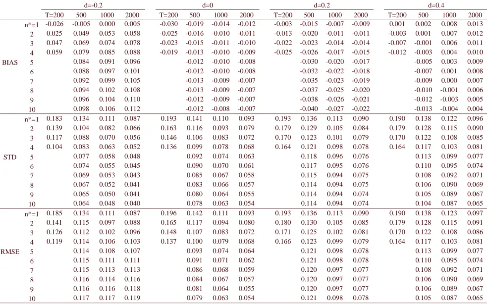
Table 1 displays bias, standard deviation and RMSE of the convex combination of GPH
estimates for n* = 1, …, 10, where the series follow ARFIMA(0,d,0) processes. When d ≥ 0,
there very little bias, if any, induced by the convex combination, while the standard deviation is
decreased by more than 40% if d = 0, by more than 25% if d = 0.2, and by about 30% if d = 0.4,
considering n* = 10. For sample size T = 200, the maximum n* equals to 4 and the reduction is
somewhat lower, although still considerable. The resulting RMSE gets reductions of same order
as the standard deviation (around 30% on average), as the bias induced is negligible. For d =
-0.2, however, the bias induced is considerable (around 0.1 for n* = 10), while the standard
deviation is reduced by almost a half. The resulting RMSE suffers at most an increase of 3% (T
= 2000), while can be reduced by about 30% for T = 200. In general, for negative values of d, the
convex combination works better for smaller samples (differently from d ≥ 0, where no great
differences were observed across sample sizes), and as the sample increases the accuracy of the
standard GPH can be no longer improved by the method.
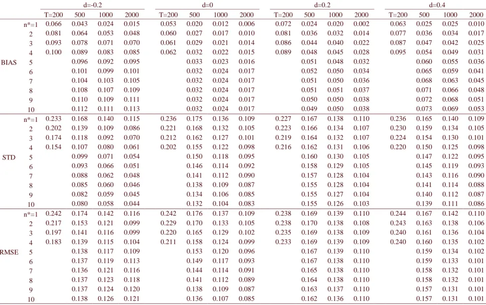
Table 2 shows the same as Table 1, but refers to the SMGPH estimator, instead of the
comparable, but quantitatively (in percentage points) slightly worse than those from the GPH if d
≥ 0. They are in general worse (especially when the sample size increases) if d < 0. For T = 2000
and d = -0.2, the RMSE is increased by about 37%, but sample sizes smaller than 1000 see
reduction in the RMSE. However, note that the RMSE of the SMGPH is lower than that of GPH,
so that is preferable to use the former in practical applications. Even in the worst case for the
convex combination applied to the SMGPH (T = 2000, d = -0.2, commented above), the RMSE
is pretty much the same as that from the convex combination applied to the GPH.
Table 3 shows the results of the convex combination applied to the GPH estimator, in the
case the data generating process (DGP) is an ARFIMA(1,d,0), with φ = 0.5. As commented in
Section 2.2, the positive AR component biases the long memory estimation upward (in
agreement with previous literature, see, for example, Bisaglia and Guégan, 1998). This bias
tends to disappear as the sample size increases. The convex combination, on the other hand,
makes this bias stronger, especially when d is negative. In addition to that, the reduction in the
standard deviation is weaker than in the case of an ARFIMA(0,d,0), if d ≥ 0 (as opposed to the
case d = -0.2, where it is decreased by more than a half for n* = 10). Even so, there are no losses
(in the squared error sense) to the original estimator if the convex combination proposed here is
applied. For d > 0, the RMSE is always decreased, but by no more than 10%. For d = 0, the
reduction is greater than 20% for n* = 10, and is of order of 15% if T = 200 and n* = 4. For d =
-0.2, the RMSE is reduced by about ¼ for T = 200 and n* = 4, but as the sample size increases,
this reduction diminishes and even turns out to be an increase of 4% when T = 2000 and n* = 10.
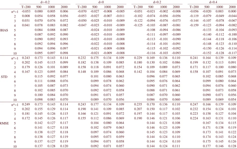
Table 4 shows the results of the convex combination applied to the GPH estimator, in the
case the DGP is an ARFIMA(0,d,1), with θ = –0.5. The negative MA, as previously commented,
biases the long memory estimation downward, this bias tending to vanish as the sample size
increases. That is because a negative MA component reduces the memory of long memory
processes (see Andersson, 2000) and makes the estimates for n>1 very close to zero (see Souza
and of opposite sign as d (negligible when d = 0), of order of 0.1 when n* = 10. On the other
hand, the standard deviation is decreased to almost a half in general when n* = 10, and decreased
to about 2/3 of its original value when T = 200 and n* = 4. The resulting RMSE is decreased to
almost a half when d = 0; while when d > 0 the result is ambiguous. When d = 0.2, the reduction
can be of 20%, decreasing with sample size until an increase of 1% when T = 2000. When d =
0.4, there is a 10% reduction for T = 200 and n* = 4, but for longer series and n* = 10 there is an
increase in the RMSE, varying from 5% to 18%, increasing with sample size. For d = -0.2, the
reduction in the RMSE decreases with sample size, going from about 30%, if T = 200 and n* =
4, to 11% when T = 1000 and n* = 10. For the longest series, T = 2000, there is actually a 5%
increase in the RMSE.
The RMSE reduction achieved by the method on the SMGPH for ARFIMA(1,d,0) and
ARFIMA(0,d,1) is not shown here, but is in general slightly worse than that obtained for the
GPH in percentage points. On the other hand, the RMSE of the SMGPH is originally lower than
that of the GPH, such that the RMSE resulting from the convex combination frequently favours
the SMGPH. It is important to point out that the technique proposed here achieves considerable
reduction in the RMSE when the DGP is an ARFIMA(0,d,0), and a smaller reduction in general
when a positive AR or negative MA (the most likely to bias the long memory estimation) of
magnitude 0.5 is present. It is noted that the greater n* used, the better result is achieved in
general, but the greater n* are likely to worsen the few unfavourable cases.
5 Concluding Remarks
In this paper, we propose a convex combination of long memory estimates taken from the
same data using different sampling rates. The Geweke and Porter-Hudak (1983) estimator and its
smoothed version are used, and the estimates from lower sampling rates must be bias corrected.
We use for this purpose the heuristic bias formula in Souza and Smith (2002), proposed for an
while introducing some bias, and the best results are in general obtained for positive values of d
(long memory). The resulting RMSE of the estimation is considerably reduced if the DGP is an
ARFIMA(0,d,0), by about 30% on average, and is in general slightly reduced when the process
is an ARFIMA (1,d,0) with φ = 0.5, or an ARFIMA (0,d,1) with θ = -0.5. The few cases were the
RMSE is only slightly increased do not justify abandoning this approach in face of the gains it
can offer.
The RMSE reduction for the ARFIMA (0,d,0) case makes it advantageous to use the
convex combination to estimate the degree of fractional integration, even taking into account the
risk of the misspecification in the bias formula.
5 References
Andersson, M. K. (2000), “Do long-memory models have long memory?”, International Journal
of Forecasting, 16, 121-124.
Bisaglia, L. & Guégan, D. (1998), “A comparison of techniques of estimation in long-memory
processes”. Computational Statistics & Data Analysis, 27, 61-81.
Chambers, M. J. (1998), “Long memory and aggregation in macroeconomic time series”,
International Economic Review 39, 1053-1072.
Crato, N. and Ray, B. K. (1996),”Model selection and forecasting for long-range dependent
processes”, Journal of Forecasting, 15, 107-125.
Geweke, J. and Porter-Hudak, S. (1983), “The estimation and application of long memory time
series models”. Journal of Time Series Analysis, 4, 221-237.
Granger, C. W. G. and Joyeux, R. (1980), “An introduction to long memory time series models
and fractional differencing”. Journal of Time Series Analysis, 1, 15-29.
Hassler, U. (1993), “Regression of spectral estimators with fractionally integrated time series”.
Journal of Time Series Analysis, 14, 369-380.
Hurvich, C. M., Deo, R. and Brodsky, J. (1998), “The mean square error of Geweke and
Porter-Hudak’s estimator of the memory parameter of a long-memory time series”, Journal of
Time Series Analysis, 19, 19-46.
Man, K. S. (2003), “Long memory time series and short term forecasts”, International Journal of
Forecasting, forthcoming.
Mandelbrot, B.B. (1977). Fractals: Form, Chance and Dimension (Freeman, San Francisco).
Ohanissian, A., Russell, J. and Tsay, R. (2003), “Using temporal aggregation to distinguish
between true and spurious long memory”, working paper, available at
http://gsb-www.uchicago.edu/fac/jeffrey.russell/research/wp.htm.
Priestley, M. B. (1981), Spectral Analysis and Time Series. London: Academic Press.
Ray, B. K. (1993), “Modeling long-memory processes for optimal long-range prediction”,
Journal of Time Series Analysis, 14, 511-525.
Smith, J., Taylor, N. and Yadav, S. (1997), “Comparing the bias and misspecification in
ARFIMA models”, Journal of Time Series Analysis, 18, 507-528.
Souza, L.R. (2003a), “The aliasing effect, the Fejer kernel and temporally aggregated long
memory processes”, working paper, available at
http://www.fgv.br/epge/home/PisDownload/1086.pdf.
Souza, L.R. (2003b), “Temporal aggregation and bandwidth selection in estimating long
memory”, working paper, available at
http://www.fgv.br/epge/home/PisDownload/1134.pdf.
Souza, L. R. and Smith, J. (2002), “Bias in the memory parameter for different sampling rates”,
International Journal of Forecasting, 18, 299-313.
Souza, L. R. and Smith, J. (2003), “Effects of temporal aggregation on estimates and forecasts of
fractionally integrated processes: A Monte Carlo study”, International Journal of
Forecasting, forthcoming.
Tschernig, R. (1995), “Long memory in foreign exchange rates revisited”, Journal of
Yamamoto, Y. and Hughson, R.L. (1991), “Coarse-graining spectral analysis: new method for
studying heart rate variability”, Journal of Applied Physiology 71, 1143-1150.
Yamamoto, Y. and Hughson, R.L. (1993), “Extracting fractal components from time series”,
Table 1: Bias, standard deviation and RMSE obtained by the method upon the GPH estimator for ARFIMA(0,d,0) processes (n*=1 corresponds to the GPH alone).
d=-0.2 d=0 d=0.2 d=0.4
18
Table 2: Bias, standard deviation and RMSE obtained by the method upon the SMGPH estimator for ARFIMA(0,d,0) processes (n*=1 corresponds to the SMGPH alone).
d=-0.2 d=0 d=0.2 d=0.4
Table 3: Bias, standard deviation and RMSE obtained by the method upon the GPH estimator for ARFIMA(1,d,0) processes, φ = 0.5 (n*=1 corresponds to the GPH alone).
d=-0.2 d=0 d=0.2 d=0.4
20
Table 4: Bias, standard deviation and RMSE obtained by the method upon the GPH estimator for ARFIMA(0,d,1) processes, θ = -0.5 (n*=1 corresponds to the GPH alone).
d=-0.2 d=0 d=0.2 d=0.4
T=200 500 1000 2000 T=200 500 1000 2000 T=200 500 1000 2000 T=200 500 1000 2000 n*=1 -0.053 0.000 0.005 0.006 -0.070 -0.027 -0.008 -0.005 -0.051 -0.021 -0.002 -0.008 -0.056 -0.020 0.003 0.000 2 0.008 0.054 0.058 0.056 -0.053 -0.027 -0.007 -0.011 -0.102 -0.074 -0.056 -0.056 -0.119 -0.079 -0.049 -0.044 3 0.031 0.070 0.076 0.072 -0.050 -0.025 -0.010 -0.009 -0.122 -0.094 -0.076 -0.073 -0.144 -0.107 -0.078 -0.067 4 0.041 0.078 0.083 0.082 -0.047 -0.023 -0.010 -0.009 -0.125 -0.103 -0.087 -0.081 -0.159 -0.123 -0.094 -0.082 BIAS 5 0.084 0.088 0.087 -0.024 -0.010 -0.009 -0.108 -0.094 -0.086 -0.133 -0.104 -0.093 6 0.087 0.092 0.090 -0.023 -0.010 -0.009 -0.111 -0.097 -0.089 -0.140 -0.112 -0.100 7 0.090 0.092 0.093 -0.023 -0.010 -0.008 -0.113 -0.101 -0.090 -0.144 -0.118 -0.106 8 0.092 0.094 0.096 -0.022 -0.010 -0.008 -0.114 -0.101 -0.091 -0.148 -0.123 -0.110 9 0.094 0.096 0.097 -0.021 -0.009 -0.008 -0.115 -0.102 -0.092 -0.150 -0.126 -0.114 10 0.095 0.097 0.098 -0.021 -0.009 -0.008 -0.116 -0.103 -0.093 -0.152 -0.128 -0.117 n*=1 0.243 0.173 0.143 0.114 0.232 0.175 0.134 0.109 0.229 0.169 0.136 0.110 0.241 0.164 0.139 0.109
✘✙✟✖☞✍✫✵✴✶✝✠✷✹✸✻✺✹✼✹✽✾❀✿★✼✹✸✻❁★✷✹❁★❂☛✼✹❃❅❄❇❆✙❈☛✷✹❁❉✕✓✾★✸✻✾❉✴❊☞✍❋☛✸✻●❍✽■❂☛✼❑❏✁▲✄▲✄❏✥✴✶✂✁✂◆▼☛❖✹P✁❃✬☎
✁✄✄☎ ☞◗✘✙✆✔✪✜❘❙✑☛✕❚✭✰✆✰❯✵✟★✘✁✕☛❱✦✭✰✘✙✆✔✿★✎✚✫❲✟❳✿☛✆✔✘❨✪✜✘✁☞✵❩❬✎✒✫◆❘✩✑✓✎✒✌✏❭❪✝✠❘❙✫❫✕✙✎✒✭✰✫✬✟❴✛❇☞✵✕☛☞❵✑❛✆✩❘✩✘✙✡✙✟★✑❴✴✞✿★✸✻✷✹❁★✺✹●❜❃✬✺✹✾
❝
☎✁❭✩☎✁✿★✼✹✸✻✸✻✼✹●❍✸✻✷❞❄✜✭✰✼❞❡✳✼✹✸❛✫✬✷✹❁✖❢❣✾★❈✖❤◆❄✜✝✠✷✹✸✐✺✹✼✹✽✾❀✌✏✼✹✸✐●❞✴❊☞✍❋☛✸✻●❍✽■❂☛✼❑❏✄▲✁▲✄❏✥✴✶✂✄❥❦▼✁❖✹P☛❃■☎
✁✄❧✄☎ ✕ ❝ ✟♠✝✠✎✚✑✓✑❛✎✚✌✣❭ ✫❲✎✚✌✣♥✄♦♣❘✩✑✓✎✒✌✏❭q✕ ❝ ✟r✌✏✪✜✟★✘ ✘✙✟★✡✙✟★✑❛✑✓✎✚✆✔✌ ✎✚✌✣✛✔✎✒✡✁☞✵✕✓✆✩✘♠✕✙✆ ✡✙✆✔✌✏✑★✕✙✘✙❘✩✡✁✕ ✡✙✆✔✎✚✌✣✡✙✎✚✛✜✟★✌✜✕❴☞✥✌✏✛s✫✬✟✖☞✍✛✜✎✚✌✣❭❨✎✒✌✏✛✜✎✚✡✓✟☛✑✠✆✔✿t✟★✡✙✆✔✌✣✆✩✝✠✎✒✡❴☞✥✡✁✕✙✎❯✵✎✕✁❱❴✴✉❆✈✾★✇✹✾✍❯✵●❍✺❞❡✳✾★✸✜✎✚❃✬❃■✽✼✹✸✒❄❙✿★✷✹✸✻❃■①★●❍❂ ❯✵✷✹①★●❍❂②✴✶✝✠✷✹●❍✾❀❂✁✼③❏✄▲✄▲✁❏✍✴✠✂✈④✥▼✁❖✹P☛❃■☎
✁✄⑤✄☎ ✑✓✭✰✟★✡✙❘✩✫✳☞✵✕✓✎❯❙✟②☞✵✕☛✕✁☞✍✡✓♥✄✑⑥✆✔✌❪✛✔✟★✪❇✕✓✑☛⑦✜✛✜✆✔✫✬✫❫☞✍✘✙✎❩✹☞✵✕✙✎✒✆✩✌✠☞✍✌✣✛✶✆✩✭■✕✓✎✚✝✠❘✩✝⑧✡✙❘❙✘✙✘✓✟☛✌✣✡✁❱◆☞✍✘✙✟✖☞✍✑❀✴ ☞✍✽✾★●❍❃■●❍✾❉☞✍✸✻✷✹❈✖❢❣✾✖❄✜✝✠✷✹✸✻✺✹●❍✷❑✫❲✼✹✾★❁❉✴✶✝✠✷✹●❍✾❀❂✁✼❑❏✁▲✄▲✁❏✍✴✶⑨✁◆▼☛❖✹P☛❃■☎
✁✄⑨✄☎ ❯✵✎✒✌✜✕☛☞✍❭✔✟❳✡✁☞✍✭✰✎✕☛☞✍✫❫⑦⑩✛✜✎✚✑★✕✙✆✔✘✁✕✓✎✚✆✔✌✏✑❳☞✍✌✏✛✞✛✜✟✖❯✵✟★✫❲✆✩✭✰✝✠✟★✌✈✕❳✴✞✑✓✷✹❶◆❈☛✼✹✽✁❂✁✼❷☞✍❋✁✸✐✼✹❈❴✭✰✼✹❃■❃■✾★✷❞❄⑩✘✓✷❞❸❹✷✹✼✹✽ ✘✙✾★❋②✴✶✝✠✷✹●❍✾❀❂✁✼❑❏✁▲✄▲✁❏✍✴✶✁✂◆▼☛❖✹P☛❃■☎
✁✄❥✄☎ ❭✩✆✰❯❙✟☛✘✓✌✏✝✠✟★✌✈✕✮☞✍✡✁✕✓✎✚✆✔✌✏✑✧✕✓✆❺✑❛❘❙✭✰✭✰✆✔✘✁✕❻✡✙✆✔✿★✿☛✟★✟❼✭✰✘✙✆✔✛✔❘✩✡✙✟★✘✙✑❽✴◗☞✍✌❾✎✚✌✈❯✵✟★✑☛✕✓✎✚❭✰☞✵✕✓✎✚✆✔✌❿✆✔✿ ✭✰✆✩✑❛✑✓✎✒✪✔✫❲✟➀✝✠✟✖☞✍✑✓❘✩✘✙✟★✑⑥✿★✘✙✆✔✝➁✕ ❝ ✟➀✟☛❘✩✘✙✆✔✭✰✟➂☞✥✌➃❘✩✌✏✎✒✆✩✌✠✴➄❭✩✼✹✸✐❶t❖✹❁➀✡✙✷✹✽❸➅✷❞❡✻❄✔✘✙✼✹❁★✷❞❡✳✾➀❭✔☎✄✿★✽➆★✸✻✼✹❃➇❆✈✸✻☎ ✴❊❆✈❈★❁★①★✾❀❂✁✼③❏✄▲✄▲✁❏✍✴✠✂✄▲❦▼✁❖✹P☛❃■☎
✁✄➈✄☎ ☞➉✝✠✆✩✛✜✟★✫➊✆✔✿❚✡✁☞✍✭✰✎✕✁☞✥✫◆☞✍✡✙✡✙❘✩✝✠❘❙✫❫☞✵✕✓✎✚✆✔✌❽☞✍✌✣✛✧✘✙✟★✌✈✕✁✱✲✑✓✟★✟★♥✄✎✚✌✣❭➃✴✧✭✰✷✹❈★✽✾s✪✜✷✹✸✻✼✹✽✽●❄③✑❛✷✹❶t❈★✼✹✽✈❂☛✼ ☞✍❋☛✸✻✼✹❈❀✭✰✼✹❃■❃✬➆☛✷✣✴❊❆✈❈★❁★①★✾❀❂✁✼❑❏✁▲✄▲✁❏✍✴✶❧✁▲◆▼☛❖✹P☛❃■☎
✁❧✄▲✄☎ ✕ ❝ ✟♠✝✠✎✚✑✓✑❛✎✚✌✣❭ ✫❲✎✚✌✣♥✄♦♣❘✩✑✓✎✒✌✏❭q✕ ❝ ✟r✌✏✪✜✟★✘ ✘✙✟★✡✙✟★✑❛✑✓✎✚✆✔✌ ✎✚✌✣✛✔✎✒✡✁☞✵✕✓✆✩✘♠✕✙✆ ✡✙✆✔✌✏✑★✕✙✘✙❘✩✡✁✕ ✡✙✆✔✎✚✌✣✡✙✎✚✛✜✟★✌✜✕❴☞✥✌✏✛s✫✬✟✖☞✍✛✜✎✚✌✣❭❨✎✒✌✏✛✜✎✚✡✓✟☛✑✠✆✔✿t✟★✡✙✆✔✌✣✆✩✝✠✎✒✡❴☞✥✡✁✕✙✎❯✵✎✕✁❱❴✴✉❆✈✾★✇✹✾✍❯✵●❍✺❞❡✳✾★✸✜✎✚❃✬❃■✽✼✹✸✒❄❙✿★✷✹✸✻❃■①★●❍❂ ❯✵✷✹①★●❍❂②✴❊❆✈❈★❁★①★✾❀❂✁✼③❏✄▲✄▲✁❏✍✴✠❏✄➈❦▼✁❖✹P☛❃■☎
✁❧✈④❲☎ ✫✬✟★✌✣✛✜✟☛✘❿✫✬✎☞✍✪✜✎✚✫❲✎✕☛❱➋✎✚✌➋✕ ❝ ✟❻✡✙✆✔✌✏✑❛❘❙✝✠✟★✘➌✡✙✘✓✟☛✛✜✎✕❿✝t☞✥✘✙♥✄✟✖✕❻✴➍✟★✽●❍❃■✷✹❋☛✼❞❡✻❡✳✷➎✎✒✾★❃■❃■✷❞❄✦❭✩●❍❈★✽●❍✷✹❁★✷ ✭✰✷✹✽❈★❶t❋☛✾❉✴❊☞✍P☛✾★❃❅❡✳✾❀❂☛✼❑❏✄▲✁▲✄❏✥✴✶❏✄▲❦▼☛❖✹P✁❃✬☎
✁❧✄❏✄☎ ✛✜✟☛✡✓✎✚✑✓✎✒✆✩✌➃✘✙❘❙✫❲✟★✑◆☞✍✌✣✛s✎✒✌✏✿★✆✔✘✙✝t☞✵✕✓✎✚✆✔✌➏✭✰✘✙✆✰❯❙✎✚✑✓✎✒✆✩✌✣♦➐✝✠✆✩✌✣✎✕✓✆✔✘✙✎✚✌✣❭✉❯❙✟★✘✙✑✓❘✩✑⑥✝t☞✍✌✣✎✚✭✰❘✩✫✳☞✵✕✓✎✚✆✔✌ ✱✵✟★✽●❍❃✬✷✹❋✁✼❞❡✻❡❫✷❑✎✚✾★❃■❃✬✷❞❄✜❭✔●❜❈★✽●❍✷✹❁★✷❑✭✰✷✹✽❈★❶◆❋✁✾❉✴❊☞✥P✁✾★❃❅❡❫✾❀❂✁✼❑❏✁▲✄▲✁❏✍✴✶✂✁⑨◆▼☛❖✹P☛❃■☎
✁❧✄✂✄☎ ✆✩✌ ✡✙✟★✘✁✕☛☞✍✎✚✌ ❭✔✟☛✆✔✝✠✟✖✕✙✘✓✎✚✡➑☞✥✑✓✭✰✟★✡✁✕✓✑➒✆✔✿➓✭✰✆✩✘☛✕✙✿★✆✔✫✬✎✒✆ ✆✔✭■✕✓✎✚✝✠✎✚✑★☞✵✕✓✎✚✆✔✌q➔❵✎✕ ❝ ❝
✎✚❭
❝
✟☛✘ ✝✠✆✩✝✠✟★✌✈✕✙✑❀✴✶❭✔❈★❃❅❡✳✷❞→➐✾❀✝✠☎✁❂✁✼✣☞✵❡✳①★✷❞➣❬❂✁✼❞❄✈✘✙✼✹❁★✷❞❡✳✾❀❭✩☎↔❸➅✽➆★✸✻✼✹❃⑩❆✙✸✻☎❲✴✠✑✓✼❞❡✳✼✹❶◆❋✁✸✻✾❀❂☛✼❑❏✁▲✄▲✄❏✥✴✶❏✙④✍▼☛❖✹P✁❃✬☎
✁❧✄✄☎ ✝✠✟★✌✏✑❛❘❙✘✁☞✍✌✣✛✜✆ ☞ ✭✰✘✙✆✩✛✜❘✩↕✁✤✍✆ ✡✙✎✚✟★✌✈✕✙➙✒✿☛✎✒✡✁☞ ✎✒✌✜✕✓✟★✘✙✌✜☞✥✡✙✎✚✆✔✌✜☞✥✫ ✟★✝ ✟★✡✙✆✔✌✣✆✩✝✠✎☞ ✛✜✟ ✭✰✟★✑✓➛✔❘❙✎✚✑★☞✍✛✜✆✩✘✓✟☛✑➜✟s✛✜✟☛✭■☞✥✘✁✕✁☞✥✝✠✟☛✌✈✕✓✆✩✑➜✪✜✘✁☞✍✑❛✎✚✫❲✟★✎✚✘✙✆✔✑❚✱✥❆✈✾★✇✹✾✉❯❙●❍✺❞❡✳✾★✸✍✎✚❃■❃✬✽✼✹✸✒❄⑩✕✓✷❞❡✳●❍✷✹❁☛✷✶✡✙✷✹✽❂✁✷✹❃ ❂✁✼③✫✬●❍❶t✷✣☞✍✺✹①★➝❑✭✰●❍✽✽✷✹✸☛✴✠✑✓✼❞❡✳✼✹❶◆❋✁✸✻✾❀❂☛✼❑❏✁▲✄▲✄❏✥✴✶✂✁➈◆▼☛❖✹P✁❃✬☎
✁❧✄❧✄☎ ✿★✆✩✘✙✟★✎✒❭✩✌❻✛✜✎✚✘✙✟★✡✁✕❼✎✒✌✜❯❙✟★✑☛✕✓✝✠✟★✌✜✕❼✑❛✭✰✎✚✫❲✫✬✆✰❯✵✟★✘✙✑❛♦✔☞✍✛✜✛✜✎✕✓✎✚✆✔✌✈☞✍✫✠✫✬✟★✑❛✑✓✆✔✌✏✑➞✿★✘✙✆✔✝➟☞➠✡✙✆✩❘✩✌✜✕✓✘✁❱ ✑☛✕✓❘❙✛❇❱⑥✱②✘✙✼✹❁★✷❞❡✳✾❳❭✩☎✓✿☛✽✾☛✸✐✼✹❃❷❆✈✸❜❄✣✝✠✷✹✸✻●❍✷❊✭✰✷✹❈★✽✷❊✿★✾★❁➂❡❫✾☛❈★✸✻✷❞❄➇✘✙✾★P✁➝✹✸✻●❍✾❴❭✔❈★✼✹✸✻✸✻✷❊✑❛✷✹❁➂❡❫✾☛❃✥✴✞✑❛✼❞❡✳✼✹❶t❋☛✸✻✾❴❂☛✼ ❏✄▲✁▲✄❏✥✴✶✂✄▲❦▼✁❖✹P☛❃■☎
✁❧✄⑤✄☎ ☞➡✡✙✆✩✌✈✕✓✘✁☞✍✡✁✕✓✎❯❙✟⑥✝✠✟✖✕ ❝ ✆✔✛➃✿★✆✔✘✦✡✙✆✔✝✠✭✰❘❬✕✓✎✚✌✣❭➄✕ ❝ ✟✉✑☛✕☛☞✵✕✓✎✚✆✔✌✜☞✍✘☛❱✞✑✓✆✔✫✬❘➐✕✙✎✒✆✩✌❽✆✩✿❀✕ ❝ ✟✉✟★❘❙✫❲✟☛✘ ✟★➛✩❘➐☞✵✕✙✎✒✆✩✌➊✱❬➔◗●❍✽❸➅✸✻✼✹❂☛✾❀✫✬☎✁✝✠✷✹✽❂✁✾★❁★✷✹❂☛✾➂❄ ❝ ❈★❶t❋☛✼✹✸✒❡✳✾❀✝✠✾★✸✻✼✹●❍✸✻✷✣✴✶✑✓✼❞❡✳✼✹❶◆❋✁✸✐✾❀❂✁✼❑❏✁▲✄▲✁❏✍✴➃④↔◆▼☛❖✹P☛❃■☎
✁❧✄⑨✄☎ ✕✙✘☛☞✍✛✜✟➢✫✬✎✒✪✜✟☛✘☛☞✍✫✬✎❩✹☞✵✕✓✎✚✆✔✌➁☞✍✌✏✛❼✕
❝
✭■☞✍❘❙✫❲✆❊✱✵✪✜✼✹✸✻❁★✷✹✸✻❂☛✾❀❂☛✼❑✑✓❖❑✝✠✾✖❡✳✷❞❄✈✝✠✷✹✸✻✺✹✼✹✽✾❀✿★✼✹✸✻❁★✷✹❁★❂✁✼✹❃➇✴✶✆✔❈➂❡❫❈☛❋☛✸✻✾❀❂☛✼❑❏✄▲✁▲✄❏✥✴✶✂✄⑨❦▼☛❖✹P✁❃✬☎
✁❧✄➈✄☎ ✿★✆✩✘✙✟★✎✒❭✩✌➜✿★❘❙✌✣✛✜✎✚✌✣❭⑥✕✙✆⑥☞✥✌➢✟★✝✠✟☛✘✓❭✩✎✒✌✏❭❨✝t☞✥✘✙♥✄✟✖✕✓♦★✕ ❝ ✟◆✝✠✆✩✌✣✟✖✕✁☞✥✘✁❱➄✭✰✘✙✟★✝✠✎✚❘✩✝❻✕ ❝ ✟★✆✔✘✁❱❴☞✍✌✣✛
✕
❝
✟➞✪✜✘✁☞✵❩❬✎✚✫❲✎☞✥✌❾✡✁☞✥✑✓✟✖⑦s④❲➈✁➈✈④✲✱❲④❲➈✁➈✄❥✞✱✠✡✙✷✹✸✻✽✾☛❃
❝
✷✹❶◆●❍✽❡✳✾★❁❚❯✵☎⑩☞✍✸✻✷✁✖❢❣✾✖❄❳✘✙✼✹❁★✷❞❡✳✾➜❭✔☎③✿★✽✾★✸✻✼✹❃✠❆✈✸✻☎⑩✴ ✆✩❈✖❡✳❈★❋☛✸✻✾❀❂☛✼❑❏✄▲✁▲✄❏✥✴✶✄⑤❦▼✁❖✹P☛❃■☎
✁⑤✄▲✄☎ ✘✙✟★✿★✆✩✘✙✝t☞❼✭✰✘✓✟➂❯❙✎✚✛✜✟★✌✣✡✙✎✗✍✘✓✎☞✍♦➐✟★✝⑧✪✜❘❙✑✓✡☛☞➞✛✜✟❦✎✒✌✏✡✓✟☛✌✈✕✓✎❯❙✆✩✑ ✭■☞✍✘✁☞❨☞✵✕✓✘✁☞✍✎✒✘➊✆❴✕✙✘✁☞✥✪✰☞✥✫
❝
☞✍✛✜✆✩✘ ☞✍❘❬✕✄✂✔✌✏✆✔✝✠✆✶✱②✑✓✷✹❶◆✷✹❁➂❡❫①☛✷③✕✓✷✹✷✹❶➠✛✜✷✹✸✒❡✐❄✣✝✠✷✹✸✻✺✹✼✹✽✾❳✡✙➆★✸✒❡✳✼✹❃◆✌✏✼✹✸✻●❄✣✿★✽✷❞→➐●❍✾❳✝✠✼✹❁★✼❞➤↔✼✹❃❷✴❪✌✣✾✖→➐✼✹❶t❋☛✸✻✾❳❂☛✼ ❏✄▲✁▲✄❏✥✴✶❏✄❥❦▼✁❖✹P☛❃■☎
✁⑤✈④❲☎ ✛✜✟☛✡✓✟☛✌✈✕❺➔◗✆✔✘✙♥➁☞✍✌✣✛ ✕
❝
✟➉✎✒✌✏✿★✆✔✘✙✝t☞✍✫➁✑❛✟★✡✁✕✙✆✔✘➋✎✚✌ ✪✜✘✁☞✵❩❬✎✚✫➞✴ ✝✠✷✹✸✻✺✹✼✹✽✾ ✡✙➆★✸✒❡✳✼✹❃➎✌✣✼✹✸✻●❀✴ ✌✏✾✖→➐✼✹❶◆❋✁✸✐✾❀❂✁✼❑❏✁▲✄▲✁❏✍✴➃④✁④❲❧❦▼✁❖✹P☛❃■☎
✁⑤✄❏✄☎ ✭✰✆✩✫❲➙✕✓✎✚✡☛☞➓✛✜✟❵✡✙✆✰✕✁☞✍✑ ✟❵✎✚✌✣✡✙✫❲❘❙✑★✤✍✆➁✕✙✘☛☞✍✪❇☞✍✫
❝
✎✚✑★✕✁☞ ✛❇☞✍✑❻✭✰✟★✑✓✑✓✆✰☞✍✑❻✡✙✆✔✝ ✛✜✟★✿★✎✚✡✙✎✆☎☛✌✣✡✙✎☞❾✱ ✝✠✷✹✸✻✺✹✼✹✽✾➊✡✓➆☛✸❜❡✳✼✹❃❳✌✏✼✹✸✻●❄✩☞✍✽✼✞✝❬✷✹❁★❂✁✸✐✼⑥✭✰●❍❁✖❡✳✾➊❂☛✼⑥✡✙✷✹✸✒→✰✷✹✽①★✾➂❄ ❝ ✼✹❃✬❃■●❍✷⑥❭✔❈★●❍✽①★✼✹✸✻❶t✾➊✡✓✾☛❃✳❡✳●❍✽✽✷➀✴➜✌✣✾➂→✰✼✹❶t❋☛✸✻✾ ❂✁✼③❏✄▲✄▲✁❏✍✴✠⑤✄⑨❦▼✁❖✹P☛❃■☎
✁⑤✄✂✄☎ ✑✓✟★✫❲✟➂✕✓✎❯❙✎✚✛❇☞✍✛✜✟♣✟➎✝✠✟★✛✜✎✚✛❇☞✍✑ ✛✜✟➎➛✔❘❬☞✍✫❲✎✚✛❇☞✍✛✜✟➎✛❇☞ ✟★✛✔❘✩✡✁☞✍↕✁✤✥✆➋✪✔✘☛☞✍✑✓✎✒✫✬✟★✎✚✘☛☞ ④↔➈✄➈✄❧↔✱❫❏✁▲✄▲✈④➃✱ ✝✠✷✹✸✻✺✹✼✹✽✾❀✡✙➆★✸✒❡❫✼✹❃✢✌✣✼✹✸✻●❄❇☞✍✽✼✞✝❬✷✹❁★❂☛✸✻✼❑✭✰●❍❁✖❡✳✾❀❂☛✼❑✡✙✷✹✸✒→➐✷✹✽①☛✾❉✴✠✌✏✾✖→➐✼✹❶◆❋✁✸✻✾❀❂☛✼❑❏✁▲✄▲✄❏✥✴✶✂✁✂✈④✥▼✁❖✹P☛❃■☎
✁⑤✄✄☎ ✪✜✘✁☞✵❩❬✎✚✫❲✎☞✥✌ ✝t☞✍✡✙✘✓✆✩✟★✡✙✆✔✌✏✆✔✝✠✎✚✡✓✑➒➔◗✎✕
❝
☞
❝
❘❙✝t☞✥✌ ✿✖☞✍✡✙✟★♦♣✝✠✟✖✕✓✘✙✆✩✭✰✆✔✫❲✎✕☛☞✍✌ ✡✓✘✙✎✚✑❛✎✚✑☛⑦ ✭✰✆➐❯❙✟★✘✁✕☛❱◆☞✍✌✣✛✠✑✓✆✔✡✙✎☞✍✫✵✕✁☞✍✘✓❭✩✟✖✕✓✑➀✴✶✝✠✷✹✸✐✺✹✼✹✽✾❀✡✙➆★✸✒❡✳✼✹❃❷✌✏✼✹✸✐●❞✴✶✌✏✾✖→➐✼✹❶◆❋✁✸✐✾❀❂✁✼❑❏✁▲✄▲✁❏✍✴✶⑤✙④✍▼☛❖✹P☛❃■☎
✁⑤✄❧✄☎ ✭✰✆✩✪✜✘✙✟✖❩✹☞✵⑦❦☞✵✕✓✎❯❙✆✩✑❻✟✮✑★☞✠✟❙✛✜✟✮✌✣✆⑧✪✜✘✁☞✍✑❛✎✚✫❚✱s✝✠✷✹✸✻✺✹✼✹✽✾✮✡✓➆☛✸❜❡✳✼✹❃➞✌✏✼✹✸✻●❄◆➔◗✷✹P✁❁★✼✹✸✉✫✬☎➀✑❛✾☛✷✹✸✐✼✹❃❚✴ ✛✜✼❞➤↔✼✹❶t❋☛✸✻✾❀❂☛✼❑❏✄▲✁▲✄❏✥✴✶❏✄➈❦▼✁❖✹P☛❃■☎
✁⑤✄⑤✄☎ ✎✚✌✣✿★✫✳☞✍↕☛✤✍✆ ✟ ✿★✫✬✟☛✡⑩✎✒✪✔✎✒✫✬✎✒✛❇☞✍✛✜✟❾✑★☞✍✫✳☞✥✘✙✎☞✍✫◗✱◗✝✠✷✹✸✻✺✹✼✹✽✾ ✡✙➆★✸✒❡✳✼✹❃➠✌✏✼✹✸✻●❄❽✝✠✷✹❈★✸✌☞❍✺✹●❍✾ ✭✰●❍❁★①★✼✹●❍✸✻✾➎✴ ✛✜✼❞➤↔✼✹❶t❋☛✸✻✾❀❂☛✼❑❏✄▲✁▲✄❏✥✴➃④❲⑤❦▼✁❖✹P☛❃■☎
✁⑤✄⑨✄☎ ✛✜✎✚✑☛✕✓✘✙✎✒✪✔❘➐✕✙✎❯✵✟❚✟☛✿★✿★✟★✡✁✕☛✕✙✑➞✆✔✿❨✪✜✘✁☞✵❩❬✎✚✫❲✎☞✥✌♣✑☛✕✓✘✙❘❙✡✁✕✓❘❙✘☛☞✍✫✠✘✙✟★✿★✆✩✘✙✝✠✑❨✱◆✝✠✷✹✸✻✺✹✼✹✽✾❚✡✙➆★✸✒❡✳✼✹❃✠✌✣✼✹✸✻●❄ ❆✈✾★❃■➝③✝✠❖✹✸✻✺✹●❍✾❀✡✙✷✹❶t✷✹✸✻P☛✾❉✴✶✛✜✼❞➤↔✼✹❶◆❋✁✸✻✾❀❂☛✼❑❏✁▲✄▲✄❏✥✴✶✂✁❥◆▼☛❖✹P✁❃✬☎
✁⑤✄❥✄☎ ✆➊✕✙✟★✝✠✭✰✆✞✛❇☞✍✑s✡✓✘✙✎☞✍✌✣↕✁☞✍✑❴✱❉✝✠✷✹✸✻✺✹✼✹✽✾❴✡✙➆★✸✒❡✳✼✹❃❦✌✣✼✹✸✻●❄⑩✛✜✷✹❁☛●❍✼✹✽✷t✡✙✾★❃❅❡✳✷✢✴✦✛✔✼❞➤➂✼✹❶t❋☛✸✻✾❴❂✁✼t❏✄▲✄▲✁❏➀✴➞④❲ ▼✁❖✹P☛❃■☎
✁⑤✄➈✄☎ ✟★✝✠✭✰✫✬✆✰❱✈✝✠✟★✌✈✕➄☞✥✌✏✛➜✭✰✘✙✆✔✛✜❘❙✡✁✕✓✎❯❙✎✕☛❱➏✎✚✌❵✪✜✘✁☞✵❩❬✎✒✫❴✎✚✌➏✕
❝
✟➊✌✣✎✚✌✣✟✖✕✙✎✒✟★✑✠✱⑩❆✙✾☛❃✬➝⑥✝✠❖✹✸✻✺✹●❍✾➊✡✓✷✹❶t✷✹✸✻P☛✾✖❄ ✝✠✷✹✸✻✺✹✼✹✽✾❀✡✙➆★✸✒❡❫✼✹❃✢✌✣✼✹✸✻●❄✜✝✠✷✹❈★✸✌☞❍✺✹●❍✾❀✡✙✾★✸✒❡✳✼❞➤✥✘✓✼✹●❜❃➇✴✶✛✜✼❞➤↔✼✹❶◆❋✁✸✻✾❀❂☛✼❑❏✁▲✄▲✄❏✥✴✶✂✁❏◆▼☛❖✹P✁❃✬☎
✁⑨✄▲✄☎ ✕ ❝ ✟✮☞✍✫❲✎☞✍✑❛✎✚✌✣❭ ✟★✿★✿★✟☛✡☛✕✁⑦ ✕ ❝ ✟♣✿★✟➂❆✙✟★✘❿♥✄✟★✘✙✌✣✟★✫➢☞✍✌✏✛➠✕✓✟★✝✠✭✰✆✩✘☛☞✍✫✬✫❫❱ ☞✍❭✩❭✔✘✙✟★❭✰☞✵✕✙✟★✛➋✫❲✆✩✌✣❭ ✝✠✟★✝✠✆✩✘✁❱⑥✭✰✘✙✆✔✡✙✟★✑✓✑❛✟☛✑❀✱❙✫✬✼✹✾★❁★✷✹✸✻❂☛✾❀✘✙☎✄✑❛✾☛❈✖➤↔✷✣✴❊❆✈✷✹❁★✼✹●❍✸✻✾❀❂☛✼❑❏✄▲✁▲✄✂✥✴✶✂✄❏❦▼✁❖✹P☛❃■☎
✁⑨✈④❲☎ ✡✙❘❙✑★✕✙✆✞✛✜✟❴✡✙✎✒✡✙✫✬✆✦✟★✡✙✆✔✌✍✂✩✝✠✎✒✡✙✆✦✌✏✆✦✪✜✘✁☞✥✑✓✎✚✫❀✟★✝❾❘❙✝❿✝✠✆✔✛✜✟★✫✬✆✦✡✙✆✔✝❿✘✓✟☛✑★✕✙✘✓✎✚↕✁✤✍✆⑥☞✧✡✙✘✏✎★✛✜✎✕✓✆ ✱✢✪✔❖✹✸✐❋✁✷✹✸✻✷➀❯✵✷✹❃✬✺✹✾★❁☛✺✹✼✹✽✾☛❃❳✪✜✾★✷❞→➐●❍❃❅❡✳✷ ❂✁✷ ✡✙❈★❁★①☛✷❞❄②✭✰✼✹❂✁✸✐✾➊✡✙✷❞→➐✷✹✽✺✹✷✹❁✖❡✳●✓✿☛✼✹✸✐✸✻✼✹●❍✸✻✷❦✴s❆✈✷✹❁★✼✹●❍✸✻✾⑥❂☛✼ ❏✁▲✄▲✁✂t✴ ❏✈④✥▼✁❖✹P☛❃■☎
✁⑨✄❏✄☎ ✕ ❝ ✟⑧✡✙✆✔✑☛✕✓✑ ✆✔✿⑧✟★✛✜❘❙✡✁☞✵✕✓✎✚✆✔✌✈⑦➜✫❲✆✩✌✣❭✩✟✖❯❙✎✕☛❱ ☞✍✌✏✛ ✕ ❝ ✟❺✭✰✆✰❯✵✟★✘✁✕☛❱ ✆✩✿❺✌✈☞✵✕✓✎✚✆✔✌✏✑❺✱❽✭✰✼✹❂☛✸✻✾ ✡✙✷❞→➐✷✹✽✺✹✷✹❁✖❡✳●✹✿★✼✹✸✻✸✐✼✹●❜✸✐✷❞❄✜✑✓✷✹❶◆❈☛✼✹✽✬❂✁✼✣☞✍❋✁✸✐✼✹❈❀✭✰✼✹❃■❃■✾★✷✏✴t❆✈✷✹❁★✼✹●❍✸✻✾❀❂✁✼③❏✄▲✄▲✁✂✍✴✠✂✈④✥▼✁❖✹P☛❃■☎
✁⑨✄✂✄☎ ☞ ❭✔✟★✌✏✟★✘✁☞✥✫✬✎❩✹☞✵✕✙✎✒✆✩✌➓✆✔✿❽❆✙❘❙✛✜✛✒✑✐✑ ✝✠✟✖✕ ❝ ✆✔✛➌✆✔✿➎✆✩❘➐✕✁✱✲✑☛✕✓✟✖☞✍✛❇❱✄✱❫✑★✕✁☞❙✕✙✟➎✡✓✆✩✝✠✭■☞✍✘✓✎✚✑✓✆✔✌✣✑⑧✎✚✌ ✭✰✟★✘✙✿★✟☛✡☛✕◗✿★✆✩✘✙✟★✑❛✎✚❭
❝
✕◗✝✠✆✔✛✜✟★✫✬✑➏✱✉✭✰✷✹❈★✽✾➃✪✔✷✹✸✐✼✹✽✽●❄❊✑❛✷✹❶t❈★✼✹✽➇❂☛✼✠☞✥❋✁✸✻✼✹❈❪✭✰✼✹❃■❃✬✾★✷✠✴➡✿★✼❞→➐✼✹✸✻✼✹●❍✸✻✾❪❂☛✼ ❏✄▲✁▲✄✂✥✴✶⑨◆▼☛❖✹P☛❃■☎
☞✍❋☛✸✻✼✹❈❀✭✰✼✹❃■❃✬✾☛✷✣✴✶✿★✼❞→➐✼✹✸✻✼✹●❍✸✻✾❀❂☛✼❑❏✄▲✁▲✄✂✥✴✶✂✄▲❦▼✁❖✹P☛❃■☎
✁⑨✄⑤✄☎ ☞ ✝✠✆✔✌✏✟✖✕☛☞✍✘✁❱❿✝✠✟★✡ ❝ ☞✥✌✏✎✒✑✓✝ ✿★✆✔✘❿✑ ❝ ☞✍✘✙✎✒✌✏❭➍✡✁☞✥✭✰✎✕☛☞✍✫✬♦⑥✛✔✎☞✍✝✠✆✔✌✏✛➉☞✥✌✏✛➌✛❇❱✙✪✰❯❙✎✚❭➋✝✠✟★✟✖✕ ♥✄✎❱✈✆✰✕✁☞✍♥✁✎↔☞✥✌✏✛t➔◗✘✓✎✚❭
❝
✕➀✴✶✘✙●❍✺✹✷✹✸✻❂☛✾❀❂☛✼❑✆✩☎✁✡✙✷❞→➐✷✹✽✺✹✷✹❁✖❡✳●❞✴✠✿☛✼❞→✰✼✹✸✻✼✹●❍✸✻✾❀❂✁✼③❏✄▲✄▲✁✂✍✴❪④❲⑤❦▼✁❖✹P☛❃■☎
✁⑨✄⑨✄☎ ✎✚✌✈☞✍✛❇☞➉✡✙✆✩✌✣✛✜✎✕✓✎✚✆✔✌✏✑➏✎✚✝✠✭✰✫❫❱❨✕ ❝ ☞✵✕➢✭✰✘✙✆✩✛✜❘✩✡✁✕✙✎✒✆✩✌➡✿★❘❙✌✣✡✁✕✙✎✒✆✩✌➡✝✠❘❙✑★✕➜✪✜✟❳☞✥✑☛❱✈✝✠✭■✕✓✆✰✕✙✎✒✡✁☞✍✫❲✫✳❱ ✡✙✆✔✪✔✪❇✱✲✛✔✆✔❘❙❭✔✫❫☞✍✑➀✱❙✭✰✷✹❈★✽✾❀✪✜✷✹✸✻✼✹✽✽●❄✜✑❛✷✹❶t❈★✼✹✽■❂☛✼✏☞✍❋☛✸✻✼✹❈❀✭✰✼✹❃✬❃■✾★✷✏✴✶✝✠✷✹✸✁✹✾❀❂☛✼❑❏✁▲✄▲✄✂✥✴✶❦▼✁❖✹P☛❃■☎
✁⑨✄❥✄☎ ✕✙✟★✝✠✭✰✆✔✘✁☞✍✫ ☞✍❭✔❭✔✘✙✟★❭➐☞✵✕✓✎✚✆✔✌ ☞✍✌✣✛ ✪❇☞✍✌✣✛✰➔❵✎✚✛❇✕ ❝ ✑❛✟★✫✬✟★✡✁✕✓✎✚✆✔✌ ✎✚✌ ✟★✑☛✕✓✎✚✝t☞❙✕✙✎✒✌✏❭ ✫❲✆✩✌✣❭ ✝✠✟★✝✠✆✩✘✁❱❦✱❙✫✬✼✹✾★❁★✷✹✸✻❂☛✾❀✘✙☎✄✑❛✾☛❈✖➤↔✷✣✱✵✝✠✷✹✸✁✹✾❀❂☛✼❑❏✁▲✄▲✄✂✥✴➃④↔➈◆▼☛❖✹P✁❃✬☎
✁⑨✄➈✄☎ ☞❺✌✣✆✰✕✙✟❨✆✔✌♣✡✙✆✔✫✬✟✉☞✍✌✏✛✧✑☛✕✓✆✩✡✙♥✁✝t☞✍✌✧✱◆✭✰✷✹❈★✽✾❨✪✜✷✹✸✻✼✹✽✽●❄❑✑✓✷✹❶t❈★✼✹✽✜❂☛✼❳☞✍❋☛✸✻✼✹❈s✭✰✼✹❃■❃■✾★✷❴✴➃☞✥❋✁✸✻●❍✽✜❂☛✼ ❏✄▲✁▲✄✂✥✴✶❥◆▼☛❖✹P☛❃■☎
✁❥✄▲✄☎ ☞
❝
✎✚✭✰✯✰✕✓✟☛✑❛✟❊✛❇☞✍✑✶✟☛✡⑩✭✰✟★✡✁✕✁☞❙✕✙✎❯❛☞✍✑✶✌✈☞✮✟★✑★✕✙✘✙❘➐✕✙❘✩✘✁☞❪☞➃✕✓✟★✘✙✝✠✆✦✛✜✟✢❆✈❘✩✘✙✆✩✑✶✌✣✆✦✪✜✘✁☞✍✑✓✎✒✫✬♦❬❘❙✝t☞ ☞✍✭✰✫❲✎✚✡✁☞✍↕☛✤✍✆➉✛✜✟➞✝✠✆✔✛✔✟★✫❲✆✩✑➡✛✜✟✦❯❬☞✍✫❲✆✩✘➁✭✰✘✙✟★✑✓✟★✌✜✕✓✟❨✱t☞✍✽✼✞✝❬✷✹❁☛❂☛✸✻✼➜✝✠✷✹●❍✷➢✡✙✾★✸✻✸✐✼✹●❜✷➏✫✬●❍❶t✷❞❄③❆✈✾★✇✹✾ ❯✵●❍✺❞❡✳✾★✸❛✎✚❃■❃✬✽✼✹✸☛✴✠✝✠✷✹●❜✾❀❂☛✼❑❏✁▲✄▲✄✂✥✴✶✂✁▲◆▼☛❖✹P✁❃✬☎
✁❥✈④❲☎ ✆✩✌❵✕
❝
✟➊➔◗✟★✫❲✿➂☞✥✘✙✟✞✡✙✆✩✑★✕✙✑❽✆✩✿✞✪✜❘❙✑❛✎✚✌✣✟★✑✓✑✧✡☛❱✈✡✙✫❲✟★✑❽✎✒✌❵✕
❝
✟✦❏✄▲❲✕
❝
✡✙✟★✌✜✕✓❘❙✘☛❱➃✱❷❆✈✾★✇✹✾⑥❯❙●❜✺❞❡❫✾☛✸ ✎✚❃✬❃■✽✼✹✸✒❄❬☞✵❸➅✾★❁★❃■✾❷☞✥✸✻●❍❁☛✾★❃❀❂☛✼◆✝✠✼✹✽✽✾t✿★✸✻✷✹❁★✺✹✾✖❄✩✆✩❃✬❶t✷✹❁★●↔✕✓✼✹●✝❬✼✹●❍✸✻✷➀❂✁✼➀✡✙✷✹✸✒→✰✷✹✽①★✾◆❭✔❈★●❜✽✽➝✹❁✍✴s✝✠✷✹●❍✾❦❂✁✼➀❏✄▲✁▲✄✂ ✴✶❏✄➈❦▼☛❖✹P✁❃✬☎
✁❥✄❏✄☎ ✘✙✟✖✕✙✆✔✘✙✌✣✆✩✑➏☞✥✌✏✆✔✘✙✝t☞✍✎✒✑❵✟➏✟★✑☛✕✓✘✁☞✵✕✄✎★❭✩✎☞✍✑❵✡✙✆✔✌✜✕✓✘✁✗✍✘✙✎☞✍✑➏✱✉✝✠✷✹✸✻✺✹✾✠☞✍❁✖❡✳✾★❁★●❜✾❪✪✜✾★❁☛✾★❶◆✾➂❄◆✎→➐✷✹❁★✷ ✛✜✷✹✽✽✑❍☞✍P☛❁☛✾★✽✳✴❊❆✈❈★❁★①★✾❀❂✁✼❑❏✁▲✄▲✁✂✍✴✶❏✁⑨◆▼☛❖✹P☛❃■☎
✁❥✄✂✄☎ ✟✖❯✵✆✔✫✬❘✩↕✁✤✍✆❪✛❇☞◗✭✰✘✙✆✔✛✔❘➐✕✙✎❯✵✎✒✛❇☞✍✛✜✟❀✕✓✆✰✕✁☞✍✫➀✛✜✆✔✑s✿✖☞✵✕✓✆✩✘✓✟☛✑➄✌✈☞❵✟★✡✙✆✔✌✏✆✔✝✠✎☞✮✪✔✘☛☞✍✑✓✎✒✫✬✟★✎✚✘☛☞✍♦✙❘❙✝t☞ ☞✍✌✈✗✍✫✬✎✒✑✓✟✉✡✙✆✔✝✠✭■☞✍✘✁☞✵✕✓✎❯❬☞➜✱✵❯❙●❜✺❞❡❫✾☛✸➇❭✔✾★❶t✼✹❃✳❄✣✑✓✷✹❶t❈★✼✹✽❇❂☛✼③☞✍❋☛✸✻✼✹❈❳✭✰✼✹❃■❃✬✾☛✷❞❄ ✿★✼✹✸✻❁★✷✹❁★❂☛✾❀☞❵☎✁❯✵✼✹✽✾☛❃✬✾❑✴ ❆✈❈★❁★①★✾❀❂✁✼❑❏✁▲✄▲✁✂✍✴✶✁❧◆▼☛❖✹P☛❃■☎
✁❥✄✄☎ ✝✠✎✚❭✔✘✁☞✍↕✁✤✥✆➐⑦✜✑❛✟★✫✬✟★↕✁✤✍✆➄✟➀✛✜✎✚✿★✟★✘✙✟★✌✏↕✁☞✥✑ ✘✙✟★❭✔✎✚✆✔✌✜☞✥✎✚✑✉✛✔✟❀✘✓✟☛✌✣✛❇☞➜✌✣✆✶✪✔✘☛☞✍✑✓✎✒✫➇✱❙✟★❁★✼✹❃❅❡✳✾★✸✓❂☛✷❑✘✙✾★❃✬✷ ❂✁✾★❃❀✑❛✷✹❁➂❡❫✾☛❃❉❆✙❈★❁☛●❍✾★✸✒❄❙✌✏✷✹➝✹✸✐✺✹●❜✾❦✝✠✼✹❁★✼❞➤↔✼✹❃❑✿★●❍✽①★✾✖❄❙✭✰✼✹❂☛✸✻✾❦✡✙✷❞→➐✷✹✽✺✹✷✹❁✖❡✳●☛✿★✼✹✸✻✸✻✼✹●❍✸✻✷②✴❳❆✈❈★❁★①★✾◆❂☛✼➀❏✄▲✄▲✁✂✢✴s❏✄✂ ▼✁❖✹P☛❃■☎
✁❥✄❧✄☎ ✕ ❝ ✟◗✘✙✎✚✑❛♥➡✭✰✘✓✟☛✝✠✎✒❘❙✝ ✆✔✌➍✪✜✘✁☞✵❩❬✎✚✫❲✎☞✥✌➟❭✔✆✰❯✵✟★✘✙✌✣✝✠✟★✌✜✕➉✛✜✟★✪✰✕☛⑦❪④↔➈✄➈✁⑤❲✱❫❏✁▲✄▲✁❏➞✱✉☞✍❁★❂✁✸✐➝✮✑✓✾★✷✹✸✻✼✹❃ ✫✬✾★❈★✸✻✼✹●❍✸✻✾✖❄✜✿★✼✹✸✻❁★✷✹❁★❂✁✾❀❂☛✼
❝
✾★✽✷✹❁★❂✁✷❑✪✜✷✹✸✻❋☛✾★❃■✷✏✱❳❆✙❈☛❁★①★✾❀❂☛✼❑❏✄▲✁▲✄✂✥✴➃④❲⑤❦▼✁❖✹P☛❃■☎
✁❥✄⑤✄☎ ✿★✆✩✘✙✟★✡✁☞✥✑☛✕✓✎✚✌✣❭➏✟★✫✬✟★✡✁✕✓✘✙✎✒✡✙✎✕☛❱✞✛✜✟★✝t☞✍✌✏✛❪❘❙✑❛✎✚✌✣❭➃❭✔✟★✌✏✟★✘✁☞✥✫✬✎❩❬✟☛✛✞✫❲✆✩✌✣❭❪✝✠✟☛✝✠✆✔✘✁❱ ✱✥✫❲✷✹✺✹●❜✸❬❆✈✾★✸✻P☛✼ ✑✓✾★✷✹✸✻✼✹❃✳❄✜✫✬✼✹✾★❁★✷✹✸✻❂☛✾❀✘✙✾★✺✹①★✷❑✑✓✾★❈✖➤↔✷✏✴❊❆✙❈★❁☛①★✾❀❂☛✼❑❏✄▲✁▲✄✂✥✴✶❏✄❏❦▼☛❖✹P✁❃✬☎
✁❥✄⑨✄☎ ❘❙✑❛✎✚✌✣❭ ✎✚✘✓✘✙✟★❭✩❘✩✫✳☞✍✘✓✫✳❱ ✑❛✭■☞✍✡✙✟★✛ ✘✙✟✖✕✙❘✩✘✙✌✏✑♠✕✙✆ ✟☛✑★✕✙✎✒✝t☞✵✕✓✟♠✝✠❘✩✫✳✕✓✎✱✲✿✖☞✍✡✁✕✓✆✩✘ ✝✠✆✔✛✜✟★✫✬✑❛♦ ☞✍✭✰✭✰✫❲✎✚✡✁☞✵✕✓✎✚✆✔✌❚✕✓✆❨✪✜✘✁☞✵❩❬✎✚✫❲✎☞✥✌➢✟★➛✩❘✩✎✕☛❱➄✛✰☞❙✕✁☞✞✱✈✗✍✽→✰✷✹✸✻✾❷❯❙✼✹●❍P✁✷❞❄❙✫✬✼✹✾★❁★✷✹✸✻❂☛✾t✘✙✾★✺✹①★✷❦✑✓✾★❈✖➤↔✷✍✴✉❆✈❈★❁★①★✾ ❂✁✼③❏✄▲✄▲✁✂✍✴✠❏✄⑤❦▼✁❖✹P☛❃■☎
✁❥✄❥✄☎ ✪✜✆✩❘✩✌✏✛✜✑✠✿★✆✩✘❊✕ ❝ ✟◆✭✰✘✙✆✔✪✰☞✥✪✔✎✒✫✬✎✕✁❱➄✛✜✎✒✑☛✕✓✘✙✎✚✪✜❘❬✕✓✎✚✆✔✌➏✿★❘✩✌✏✡✁✕✓✎✚✆✔✌➏✆✔✿✥✕ ❝ ✟◆✫❲✎✚✌✣✟✖☞✍✘t☞✍✡✙✛➄✭✰✘✙✆✔✡✙✟★✑✓✑ ✴✶✝✠✷✹✸✻✺✹✼✹✽✾❀✿★✼✹✸✻❁★✷✹❁★❂☛✼✹❃⑩✴❊❆✙❈★✽①★✾❀❂✁✼❑❏✁▲✄▲✁✂✍✴➃④↔▲◆▼☛❖✹P☛❃■☎