Sub-daily variability of suspended sediment fluxes in small mountainous catchments – implications for community-based river monitoring

(1)

HESSD

7, 8233–8263, 2010

Sub-daily variability of suspended sediment fluxes

C. Duvert et al.

Title Page

Abstract Introduction

Conclusions References

Tables Figures

◭ ◮

Back Close

Full Screen / Esc

Printer-friendly Version Interactive Discussion

Discussion

P

a

per

|

Dis

cussion

P

a

per

|

Discussion

P

a

per

|

Discussio

n

P

a

per

Hydrol. Earth Syst. Sci. Discuss., 7, 8233–8263, 2010 www.hydrol-earth-syst-sci-discuss.net/7/8233/2010/ doi:10.5194/hessd-7-8233-2010

Hydrology and Earth System Sciences Discussions

This discussion paper is/has been under review for the journal Hydrology and Earth System Sciences (HESS). Please refer to the corresponding final paper in HESS if available.

Sub-daily variability of suspended

sediment fluxes in small mountainous

catchments – implications for

community-based river monitoring

C. Duvert1, N. Gratiot1, J. N ´emery2, A. Burgos3, and O. Navratil4

1

Laboratoire d’ ´etude des Transferts en Hydrologie et Environnement (LTHE), UMR5564, Universit ´e de Grenoble/IRD, Grenoble, France

2

Laboratoire d’ ´etude des Transferts en Hydrologie et Environnement (LTHE), Universit ´e de Grenoble/G-INP, Grenoble, France

3

Centro de Investigaciones en Geograf´ıa Ambiental (CIGA), Universidad Nacional Aut ´onoma

de M ´exico, Morelia, Mexico

4

Cemagref, Unit ´e de recherche ´Erosion Torrentielle, Neige et Avalanches (ETNA),

(2)

HESSD

7, 8233–8263, 2010

C. Duvert et al.

Title Page

Tables Figures

◭ ◮

Back Close

Full Screen / Esc

Discussion

P

a

per

|

Dis

cussion

P

a

per

|

Discussion

P

a

per

|

Discussio

n

P

a

per

|

Received: 11 October 2010 – Accepted: 13 October 2010 – Published: 19 October 2010

Correspondence to: C. Duvert (clement.duvert@gmail.com)

(3)

HESSD

7, 8233–8263, 2010

C. Duvert et al.

Title Page

Tables Figures

◭ ◮

Back Close

Full Screen / Esc

Discussion

P

a

per

|

Dis

cussion

P

a

per

|

Discussion

P

a

per

|

Discussio

n

P

a

per

Abstract

Accurate estimates of suspended sediment yields depend on effective monitoring strategies. In mountainous environments undergoing intense seasonal precipitation, the implementation of such monitoring programs relies primarily on a rigorous study of the temporal variability of fine sediment transport. This investigation focuses on sea-5

sonal and short-term sediment variability in a subhumid region of the Mexican Volcanic Belt. Intensive hydrosedimentary monitoring was conducted during one year on four contrasting catchments (3 to 630 km2). Analyses revealed significant temporal variabil-ity in suspended sediment export over various time scales, with between 63 and 97% of the annual load exported in as little as 2% of the time. Statistical techniques were 10

used to evaluate the sampling frequency required to get reliable annual sediment yield estimates at the four sites. A bi-daily sampling would be required at the outlet of the 630-km2catchment, whereas in the three smaller catchments (3–12 km2), the achieve-ment of accurate estimates would inevitably require hourly monitoring. At the larger catchment scale, analysis of the sub-daily variability of fine sediment fluxes showed 15

that the frequency of sampling could be lowered by up to 100% (i.e. from bi-daily to daily) if considering a specific and regular sampling time in the day. In contrast, con-ducting a similar sampling strategy at the three smaller catchments could lead to seri-ous misinterpretation (i.e. up to 1000% error). Our findings emphasise the importance of an analysis of the sub-daily variability of sediment fluxes in mountainous catchments. 20

Characterising this variability may offer useful insights for improving the effectiveness of community-based monitoring strategies in rural areas of developing countries. In regions where historical records based on discrete sampling are available, it may also help assessing the quality of past flux estimates. Finally, the study confirms the global necessity of acquiring more high frequency data in small mountainous catchments, 25

(4)

HESSD

7, 8233–8263, 2010

C. Duvert et al.

Title Page

Tables Figures

◭ ◮

Back Close

Full Screen / Esc

Discussion

P

a

per

|

Dis

cussion

P

a

per

|

Discussion

P

a

per

|

Discussio

n

P

a

per

|

1 Introduction

Mountainous subcatchments are known to produce high amounts of fine sediment, because of their steep and incised morphology (Dietrich and Dunne, 1978; Walling and Webb, 1996; Sidle et al., 2000). It is therefore essential to provide accurate sediment flux estimates within these spatially-reduced areas, in order to quantify soil loss and 5

eventually to implement adapted land conservation practices.

De Boer et al. (2003) recently a_ffirmed that “[. . . ] in many parts of the world, ero-sion rates and sediment yields are not, or only poorly, monitored. This problem is particularly evident in developing countries, where this information is most urgently required [. . . ]”. To offset the data scarcity affecting developing countries, a number 10

of prediction methods have been applied to ungauged basins (e.g. Morehead et al., 2003). However, such techniques are not satisfying in smaller catchments charac-terized by highly-scattered and unpredictable relations between suspended sediment concentration (SSC) and discharge (Q) (Horowitz, 2008). In these situations, direct and adapted measurements are the only manner to estimate annual exports of fine 15

sediment (Walling et al., 2003).

In Mexico, the effort has historically been focused on lakes and larger basins, and still very few mountainous catchments are instrumented, despite strong erosion and water quality problems (Alcocer and Bernal-Brooks, 2010). Natural resources in the rural ar-eas of the country are commonly managed by organised local communities (Vel ´azquez 20

et al., 2003; Bocco et al., 2005). The interest of local stakeholders and citizens in water-related issues is undeniable, as recently outlined by Ortiz- ´Avila (2009) in the Michoac ´an state. This inquiry showed that water contamination and drinking water were among the main environmental priorities of local communities. A few planning initiatives for wa-ter quality monitoring are currently being developed in the country (Aranda et al., 2008; 25

(5)

HESSD

7, 8233–8263, 2010

C. Duvert et al.

Title Page

Tables Figures

◭ ◮

Back Close

Full Screen / Esc

Discussion

P

a

per

|

Dis

cussion

P

a

per

|

Discussion

P

a

per

|

Discussio

n

P

a

per

increasingly more prevalent in the last decade (e.g. Whitelaw et al., 2003; Deutsch and Orprecio, 2005; Sharpe and Conrad, 2006; Fernandez-Gimenez et al., 2008). Such approaches could be usefully implemented in Mexico, given that the involvement of lo-cal volunteers in river monitoring could allow gathering of data in ungauged catchments in a cost-e_fficient way. Furthermore, suspended sediment yield (SSY) measurements 5

should systematically be included in these participatory surveys. SSY data are in-deed of local interest in rural areas for the identification of a range of in-catchment processes, i.e. soil loss rates from cultivated land, useful life of reservoirs, monitoring of sediment-associated contaminants, etc.

A lot of work has been done worldwide on SSY estimates and on sediment ex-10

port seasonal and daily variability within mesoscale to large river basins (e.g. Ongley et al., 1977; Walling and Webb, 1981; Milliman and Syvitski, 1992; Meybeck et al., 2003). Errors and bias in SSY estimates associated with sampling frequency have also been extensively characterised for 103 to 106km2 basins (de Vries and Klavers, 1994; Phillips et al., 1999; Horowitz, 2003; Coynel et al., 2004; Moatar et al., 2006). 15

However, very few studies have addressed the question of sub-daily variability within smaller catchments (Mano et al., 2009). Meybeck et al. (2003) only pointed out that SSC variability within catchments under 10 km2 had to be established at fine time-scales such as a few hours. But the consequences of an inadequate sampling design, including the choice of an inappropriate sampling time during the day, have, to date, 20

been little debated by the scientific community (Mano et al., 2009; Moatar et al., 2009). A better characterisation of the sub-daily variability of sediment fluxes in mountainous catchments is therefore required to improve the efficiency of present-day river monitor-ing. Additionally, in areas where SSC has been routinely sampled over a number of decades, quantifying suspended sediment short term variability can be useful for as-25

(6)

HESSD

7, 8233–8263, 2010

C. Duvert et al.

Title Page

Tables Figures

◭ ◮

Back Close

Full Screen / Esc

Discussion

P

a

per

|

Dis

cussion

P

a

per

|

Discussion

P

a

per

|

Discussio

n

P

a

per

|

A near-continuous monitoring of streamflow and suspended sediment fluxes was conducted in contrasting mountainous catchments (3–630 km2) of the Mexican High-lands. In this paper we aim to provide answers to the following questions: (1) how significant is the seasonal variability in streamflow and suspended sediment, and are there sub-daily fluctuations in the hydrosedimentary regime of the studied streams? 5

(2) Is the effect of sampling frequency quantifiable, and is it site- or size-dependent? (3) Can we deduce relevant community-based monitoring strategies for such moun-tainous catchments?

2 Methods

2.1 Study site

10

The Cointzio basin is located in the southern part of the Mexican Central Plateau, within the Transverse Volcanic Belt (Fig. 1). The region undergoes a temperate subhumid climate characterised by two contrasting seasons: the dry season from November to May and the wet season between June and October. Mean annual rainfall reaches 770 mm in Morelia. Nearly 80% of the precipitation occurs during the five months of the 15

rainy season (Carl ´on-Allende et al., 2009). Rainfall is characterised by a high sub-daily variability, with localised convective storms generally promoting intense precipitation over a few km2in the late afternoon through early night.

The Cointzio basin drains an area of 630 km2with altitudes from 3440 m at the high-est point to 1990 m at the outlet. The main watercourse is theRio Grande de Morelia

20

river, which reaches the man-made reservoir of Cointzio (4 km2, 65 Mm3) at the outlet of the catchment. The geology mainly consists of basalt and andesitic rocks. Soils are finely textured; Andisols are prominent in upland parts of the basin, Acrisols on the hillslopes and Luvisols in the lowlands (FAO, 2006).

Sediment exports were measured at the outlet of the Cointzio catchment (Undameo 25

(7)

HESSD

7, 8233–8263, 2010

C. Duvert et al.

Title Page

Tables Figures

◭ ◮

Back Close

Full Screen / Esc

Discussion

P

a

per

|

Dis

cussion

P

a

per

|

Discussion

P

a

per

|

Discussio

n

P

a

per

contrasting landforms, morphologies and soil types (more details can be found in Duvert et al., 2010). High frequency water discharge data were acquired from Jan-uary 2008 to JanJan-uary 2010 in Undameo (630 km2) and in Potrerillos (12 km2), and from January 2009 to January 2010 in the two other subcatchments, i.e. La Cortina (9 km2) and Huertitas (3 km2). Suspended sediment measurements were conducted 5

from January 2009 to January 2010 at all stations. Hydrosedimentary fluxes could therefore be estimated all throughout 2009 at the four sites.

2.2 Field sampling and flux estimates

2.2.1 At the outlet

Historical monitoring of the gauging station of Undameo was launched in 1939 by the 10

Comisi ´on Nacional del Agua (CONAGUA). At that time a Parshall flume was built to provide a control of the hydraulic section. A stage-discharge rating curve was also established and regularly adjusted. Daily measurements of both water level and SSC were manually conducted by the CONAGUA from 1939 to 2002. For this research, water level was surveyed at a 5-min time-step with a Thalimede OTT water level gauge. 15

Water discharge time series were then determined via the CONAGUA rating curve. Turbidity was automatically measured every 10 min with a WTW Visolid 700-IQ neph-elometric sensor using infrared backscattering. Various authors (e.g. Gippel, 1995; Lewis, 1996) showed that continuous time-series of SSC can be efficiently derived from continuous turbidity series if the calibration is frequently adjusted. Indeed, a num-20

ber of parameters govern the disparities between SSC and turbidity, such as variation in sediment size or colour. 314 samples were collected all throughout 2009, covering both storms and baseflow conditions. This manual sampling was conducted by local families on a daily basis at approx. 07:00 p.m. Calibration of the turbidimeter proved to remain steady during the entire period. We therefore used the same rating curve 25

(8)

HESSD

7, 8233–8263, 2010

C. Duvert et al.

Title Page

Tables Figures

◭ ◮

Back Close

Full Screen / Esc

Discussion

P

a

per

|

Dis

cussion

P

a

per

|

Discussion

P

a

per

|

Discussio

n

P

a

per

|

Annual SSYref(Mg y− 1

) was obtained from the continuous time series and was used as reference value in this study. It was calculated using the following formula:

SSYref= n

Z

i=1

SSFd t with SSF=SSC·Q·10−3 (1)

where SSF is the instantaneous suspended sediment flux (Mg s−1_{), SSC is the}

in-stantaneous suspended sediment concentration (g l−1) (10-min frequency interpolated 5

to 5-min),Q is the instantaneous discharge (m3s−1) (5-min frequency), and n is the number of 5-min intervals included in a year.

It should be noted that SSY estimates cumulate uncertainties on both SSC and discharge measurements (Lewis and Eads, 2008; Navratil et al., 2010).

2.2.2 At the three subcatchments

10

Water level was surveyed at a 5-min time-step with the same gauging material as at the catchment’s outlet. In each station, discharge measurements were previously carried out at various stage levels using the NaCl tracer dilution gauging method. Discharge time series were determined from water level continuous records through the rating curve. SSC time series were calculated using stage-triggered Teledyne ISCO 3700 15

automatic water samplers containing 24 bottles of 1 l each. Sampling regime during most of the stormflow events reached a 5-min frequency. Further details about the methodology can be found in Duvert et al. (2010).

Collected samples were filtered in the laboratory of CIGA-UNAM in Morelia. The preweighed filters (pore diameter, 0.7 µm) were dried for 2 h at 105◦_{C and weighed}

20

(9)

HESSD

7, 8233–8263, 2010

C. Duvert et al.

Title Page

Tables Figures

◭ ◮

Back Close

Full Screen / Esc

Discussion

P

a

per

|

Dis

cussion

P

a

per

|

Discussion

P

a

per

|

Discussio

n

P

a

per

In the three subcatchments, annual SSY_refwere calculated following Eq. 1 by using a 5-min interpolation of SSC data obtained from the monitoring. We considered that SSF measured at the three subcatchments through automatic sampling could be assimi-lated to a high frequency survey. A large majority of the storms was indeed sampled continuously throughout the season (i.e. 5-min frequency), and the less-sampled base-5

flow fluxes did not represent a significant part of overall fluxes: based on regular manual sampling conducted during recession phases, baseflow contributed 18 Mg km−2out of 900 Mg km−2(i.e. 2% of total flux) in Huertitas, 4 Mg km−2 out of 600 Mg km−2(i.e. un-der 1% of total flux) in Potrerillos, and 1 Mg km−2 out of 30 Mg km−2 (i.e. 3% of total flux) in La Cortina.

10

Various metrics were also calculated at each station to assess the seasonal dynam-ics of suspended sediment transport. Ms2% corresponds to the percentage of annual SSY discharged in 2% of time (i.e. approx. 7 days);Ts50% refers to the percentage of time needed to carry 50% of the annual SSY (Meybeck et al., 2003).

2.3 Sub-sampling simulations

15

Following the methodology previously reported by Phillips et al. (1999), Coynel et al. (2004), Moatar et al. (2006), and Mano (2008), we intended to assess the effect of infrequent sampling on the accuracy of annual yield estimates. Various sampling fre-quencies were therefore simulated by extracting instantaneous SSC values and their corresponding discharges from the high frequency data. Simulations were conducted 20

using the following sampling designs: monthly (S1), fortnightly (S2), weekly (S3), every 3 days (S4), daily (S5), every 12 h (S6), every 6 h (S7), every 3 h (S8) and hourly (S9) frequencies. Subsequent simulated yields were calculated according to “Method 15” described by Phillips et al. (1999):

SSYsim=K ns

X

i=1

(C_i_·Q_i) (2)

(10)

HESSD

7, 8233–8263, 2010

C. Duvert et al.

Title Page

Tables Figures

◭ ◮

Back Close

Full Screen / Esc

Discussion

P

a

per

|

Dis

cussion

P

a

per

|

Discussion

P

a

per

|

Discussio

n

P

a

per

|

whereC_i andQ_i are respectively the instantaneous SSC and discharge values at the time of sampling, ns is the number of samples taken in a year (ns ranges between 12 for S1 and 8760 for S9) andK is a conversion factor depending on the sampling frequency.

For each scenario, all possible simulations were performed, i.e. 8640 combinations 5

for scenario S1, 4320 for S2, 2016 for S3, 864 for S4, 288 for S5, 144 for S6, 72 for S7, 36 for S8, and 12 for S9. Annual SSY obtained from the continuous monitoring were then used as the reference values against which the accuracy of the simulated scenarios was assessed through relative error calculations.

The sub-daily variability of SSY was also analysed. The 288 values recorded each 10

day were therefore separated into 24 groups in order to account for the hour of sam-pling in the simulations. S5 scenario (i.e. daily samsam-pling frequency) was run 24 times considering every sampling time from 00:00 a.m. to 11:00 p.m. These 24 scenarios are referred to in the text as S5₀, S5₁, . . . , S5₂₂, S5₂₃. For each of the S5_i scenarios, 13 simulations were considered, corresponding to a 1 h data interval centred on the 15

assessed sampling time. The resulting errors on annual yield estimates were then calculated for every S5_i scenario and are discussed in Sect. 3.5.

3 Results and discussion

3.1 Streamflow dynamics

On average, 29 storm events were recorded at each monitoring station throughout 20

2009. We therefore hypothesised that these sampled events were statistically rep-resentative of the general hydrosedimentary behaviour prevailing in the four studied streams. Furthermore, when compared to long term records available at the outlet of the 630-km2 basin, it appears that 2009 was an average year considering pre-cipitation: total rainfall depth measured in Cointzio during 2009 reached 805 mm, 25

(11)

HESSD

7, 8233–8263, 2010

C. Duvert et al.

Title Page

Tables Figures

◭ ◮

Back Close

Full Screen / Esc

Discussion

P

a

per

|

Dis

cussion

P

a

per

|

Discussion

P

a

per

|

Discussio

n

P

a

per

400–1100 mm y−1 (Gratiot et al., 2010). Mean discharge, however, only reached 1.3 m3s−1in 2009, which was one of the lowest values in more than 60 years.

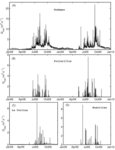
The primary factor in controlling river flow variability was the meteorological season-ality affecting the region. This pattern is well exemplified in Fig. 2, which shows the discharge records acquired between January 2008 and December 2009 in both Un-5

dameo (Fig. 2a) and Potrerillos (Fig. 2b), as well as the discharge records acquired throughout 2009 in both La Cortina (Fig. 2c) and Huertitas (Fig. 2d). The succession of wet and dry periods is visually obvious. This well-defined cycle was observed in all the studied areas. Still, it was more pronounced in the three upland catchments, mainly because of the sustained lower baseflow in upstream areas than in lowland 10

plains during the dry season.

Regarding hydrological regimes during floods, the three subcatchments exhibited very responsive behaviours (Fig. 2b, c, d), with nearly instantaneous rising phases followed by rather short recession limbs (Duvert et al., 2010). Flood durations at the outlet of the 630-km2 catchment (Fig. 2a) were significantly longer (average of 9 h) 15

than within upland areas (average of 1 h in Huertitas to 3 h in Potrerillos). In 2009, annual specific instantaneous peak discharges ranged as follows: 0.13 mm h−1in Un-dameo, 2.5 mm h−1 _{in Potrerillos, 2.9 mm h}−1 _{in La Cortina and 10.8 mm h}−1 _in

Huer-titas. Annual mean specific discharges q∗ were also calculated at the four stations, with values ranging from 4×10−3mm h−1 in Potrerillos, 7×10−3mm h−1 in Undameo,

20

to 22×10−3mm h−1 in La Cortina and 32×10−3mm h−1 in Huertitas. These values

outline the heterogeneity in the hydrological response of each of the catchments. Significant discrepancies were evidenced in the streamflow regimes of the four mon-itored catchments. Annual instantaneous peak discharges were inversely related to catchment sizes, most likely because smaller areas statistically receive higher amounts 25

(12)

HESSD

7, 8233–8263, 2010

C. Duvert et al.

Title Page

Tables Figures

◭ ◮

Back Close

Full Screen / Esc

Discussion

P

a

per

|

Dis

cussion

P

a

per

|

Discussion

P

a

per

|

Discussio

n

P

a

per

|

3.2 Seasonal and daily dynamics of SSY

Annual SSY reached 900 Mg km−2in Huertitas (low estimate), 600 Mg km−2in Potreril-los (low estimate) and 30 Mg km−2in La Cortina (Duvert et al., 2010). At the outlet of the Cointzio catchment (Undameo station), SSY was estimated at 45 Mg km−2. Accord-ing to the classification proposed by Meybeck et al. (2003), annual SSY were “medium” 5

in Undameo and La Cortina and “very high” in Potrerillos and Huertitas. Catchment characteristics such as land cover, steepness and degree of land degradation were the prevailing factors in explaining suspended solid yields discrepancies.

Given the strong seasonality observed in streamflow records, we aimed to check whether hydrosedimentary regime was characterised by a comparable variability. 10

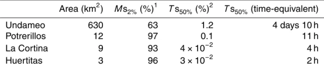
Some typical metrics were therefore calculated, and the duration curves of annual SS flux were produced for each site (these curves were obtained by displaying the percent of SS flux versus the percent of time). According to Fig. 3 and Table 1, half of the an-nual load (Ts50%) was carried in less than 0.1% to 1.2% of time, and in 7 days (Ms2%) the rivers exported between 63 and 97% of annual flux. The highest variability was 15

observed in Huertitas and the lowest in Undameo.

Meybeck et al. (2003) calculated theMs2%of several small basins (64–500 km 2

) from their global database, and they found values reaching 50 to 90%. Mano et al. (2009) observed Ms_2% values ranging from 38 to 84% in four small to medium-sized catch-ments of the French Alps. Therefore, our results are comparable with those previous 20

studies. According to theTs50% andMs2% indicators, the sediment flux duration pat-terns ranged from “very short” in Undameo to “extremely short” in Potrerillos, La Cortina and Huertitas (Table 1). This outlines the predominant contribution of a few extreme floods in the annual SSY of these highly responsive basins, as already reported by several authors worldwide (e.g. Syvitski and Morehead, 1999; Meybeck et al., 2003; 25

(13)

HESSD

7, 8233–8263, 2010

C. Duvert et al.

Title Page

Tables Figures

◭ ◮

Back Close

Full Screen / Esc

Discussion

P

a

per

|

Dis

cussion

P

a

per

|

Discussion

P

a

per

|

Discussio

n

P

a

per

3.3 Influence of sampling frequency on SSY estimates

The results obtained from the nine sub-sampling simulations (S1 to S9) are presented in Fig. 4. Figure 4a outlines the maximum errors obtained among all simulations on an-nual yield estimates for each scenario (vertical axis) and for each catchment (horizontal axis). If we consider that a deviation between simulated and reference yield estimates 5

falling within the±20% range is acceptable in terms of reliability (Navratil et al., 2010),

the minimum sampling frequencies would be for Undameo a bi-daily sampling strat-egy (i.e. S6 scenario), whereas for the three subcatchments an hourly sampling (i.e. S9 scenario) would be needed (Fig. 4a). Imprecision was much more significant in the three subcatchments than in the whole basin; again, this is an evidence for scale 10

effects. For instance, if considering a bi-daily sampling (i.e. S6 scenario), maximum er-rors on annual yield estimate could reach 17% in Undameo, 240% in Potrerillos, 420% in La Cortina and up to 540% in Huertitas.

Figure 4b shows the relative errors between the upper or lower quartile of each simulation and the reference fluxes (the selected quartile value was the one of the two 15

falling furthest from the median). At every site, the errors on flux estimates decreased significantly with increasing sampling frequencies. Based on the analysis of Fig. 4b, the adapted sampling frequency could be lowered to 3 h in La Cortina and Potrerillos.

Figure 4c presents the distribution of errors between the median values of each simulation and the reference fluxes. A systematic negative bias was observed in the 20

median values of S1 to S4 scenarios in Undameo and in the median values of S1 to S7 scenarios in the three upland catchments. This bias was related to the temporal non-linearity of sediment fluxes, as illustrated in Fig. 3.

Despite corresponding to the most probable scenarios, the information provided in Fig. 4c has to be regarded as an optimistic picture, given that the distribution of errors 25

(14)

HESSD

7, 8233–8263, 2010

C. Duvert et al.

Title Page

Tables Figures

◭ ◮

Back Close

Full Screen / Esc

Discussion

P

a

per

|

Dis

cussion

P

a

per

|

Discussion

P

a

per

|

Discussio

n

P

a

per

|

“worst case” scenarios, and basing a sampling design on those results can be thought of as a more secure, though more time constraining, approach.

Whatever the error considered (i.e. maximum, quartile or median), the minimum monitoring frequency required to get reliable sediment yield estimates was found to be highly size-dependent (Fig. 4). This can be explained by the high temporal variability 5

of discharge and SSC concentrations, because of the shorter and flashier nature of floods in the upland subcatchments as compared to the larger Cointzio catchment. A similar pattern has been observed by Horowitz (2008) for catchments of contrasting sizes (1×103to 5×104km2) in North America. On the whole, reliable SSY estimates

in small mountainous catchments appeared to require very high sampling frequencies. 10

3.4 Sub-daily variability in SSY

Given the particular characteristics of rainfall in the region (i.e. precipitation activity gen-erally peaking in late afternoon to early night), the potentially resulting sub-daily vari-ability in SSY was assessed. We therefore analysed the distribution of suspended sed-iment exports all throughout the day and on an hourly basis. The distribution of events 15

along the day was also determined by counting all peak flow occurrences included in each 1-h time interval. The results are detailed in Fig. 5. In Undameo (Fig. 5a), fluxes were distributed irregularly during the day, with higher loads discharged during the night and lower loads during the day. The peak in export occurred around midnight (ca. 30% of the total yield exported in 5 h). At the three subcatchments (Fig. 5b, c, d), 20

the temporal variability in sediment export was much more significant. Conditions with high SS fluxes prevailed during the late afternoon. In Potrerillos (Fig. 5b), almost all the SSY (i.e.>85%) occurred between 05:00 p.m. and 03:00 a.m. In La Cortina (Fig. 5c), over 90% of sediment was exported between 05:00 p.m. and midnight. In Huertitas (Fig. 5d), the bulk of sediment (i.e.>60%) reached the outlet between 03:00 p.m. and 25

(15)

HESSD

7, 8233–8263, 2010

C. Duvert et al.

Title Page

Tables Figures

◭ ◮

Back Close

Full Screen / Esc

Discussion

P

a

per

|

Dis

cussion

P

a

per

|

Discussion

P

a

per

|

Discussio

n

P

a

per

Overall, sub-daily variability in SSY proved to be very significant. Again, this vari-ability was closely related with catchment size: our results show that the fluctuations in sediment response were much larger in upstream catchments than in the entire basin. We therefore hypothesise that such temporal variability may have critical conse-quences on the manual sampling strategies to be implemented.

5

3.5 Benefits of an adapted sampling time

Errors on yield estimates associated with a change in daily sampling time were as-sessed by simulating S5₀ to S5₂₃ scenarios. The results are presented in Fig. 6. At all sites, sampling time revealed to have a significant effect on flux estimate uncertain-ties. In Undameo (Fig. 6a), annual SSY was clearly underestimated or overestimated 10

depending on the timing selected. For instance, daily sampling at night would lead to a positive bias of ca. 50%, whereas daily sampling in the afternoon would provide an underestimation of ca.−50%. In contrast, other time intervals would generate rather

accurate yield estimates: the window ranging from early morning to midday maintained the error within the±20% range. This finding is of high importance in the perspective

15

of implementing manual sampling strategies, as it could allow lowering the sampling frequency by 100% (i.e. shifting from S6 to an adapted S5). Furthermore, the daily sampling conducted by local sta_ff throughout 2009 around 07:00 p.m. led to a “real” SSY estimate of 56 Mg km−2. It corresponds to a positive bias of 25% in comparison to the reference flux. This result is in agreement with the slight overestimation that was 20

provided by S5₁₉ scenario on yield estimates, as outlined in Fig. 6a.

At the three subcatchments (Fig. 6b, c, d), the influence of SSC sub-daily variability was even more obvious, as previously expected by the analysis of Fig. 5. In La Cortina (Fig. 6c), daily sampling in the early morning to mid-afternoon would give a moderate to strong underestimation of SSYref(minimum−100%). Then, from late afternoon to early 25

(16)

HESSD

7, 8233–8263, 2010

C. Duvert et al.

Title Page

Tables Figures

◭ ◮

Back Close

Full Screen / Esc

Discussion

P

a

per

|

Dis

cussion

P

a

per

|

Discussion

P

a

per

|

Discussio

n

P

a

per

|

and Potrerillos (Fig. 6b) was similar to the one described in La Cortina, with the periods of flux overestimation slightly differing from one area to another: in Huertitas the “flood-ing” period occurred during the afternoon and in Potrerillos it was significantly more extended (i.e. from mid-afternoon to night). At the three sites, the choice of a sampling time during those periods would systematically provide very high uncertainties and im-5

precision of the estimates. In turn, this could lead to seriously biased interpretations of sediment transport within these small catchments.

3.6 Towards an optimised community-based monitoring strategy

We showed for the studied catchments that a high probability of systematic under-estimation exists if the sampling frequency is not adapted. According to the classic 10

randomly-based study of sampling frequency, a bi-daily sampling would be required at the outlet of the Cointzio basin (Undameo, 630 km2). However, this frequency could be lowered to a daily survey if considering a specific and regular sampling time window in the day (i.e. from early morning to midday), as outlined in Sect. 3.5.

In the three smaller catchments, the achievement of reliable SSY estimates proved 15

to require very high sampling frequencies, i.e. hourly monitoring. We also showed that if considering a daily survey, even the use of a specific sampling time would lead to strong biases on annual sediment yield estimates (Fig. 6). This is particularly true if the time selected is concomitant with the period when floods are most likely to occur. For instance, a daily sampling in the afternoon in Huertitas could lead to a positive bias 20

of up to 1200%. This can be explained by the very short nature of events in these small areas (1 to 3 h): whatever the method considered (linear, nearest-neighbour, etc.), the interpolation of an instantaneous measurement taken during a flood to a daily flux inevitably leads to a substantial SSY overestimation. Trying to estimate annual yield by collecting samples during floods would thus be a counterproductive approach.

25

(17)

HESSD

7, 8233–8263, 2010

C. Duvert et al.

Title Page

Tables Figures

◭ ◮

Back Close

Full Screen / Esc

Discussion

P

a

per

|

Dis

cussion

P

a

per

|

Discussion

P

a

per

|

Discussio

n

P

a

per

Nonetheless, rising stage samplers might be considered as a potential substitute for suspended sediment monitoring. They have been used in recent literature (e.g. Kostaschuk et al., 2003; Francke et al., 2008), and could be implemented in small mountainous catchments where automated instrumentation is not feasible for mone-tary constraints. Yet, this sampling alternative requires further testing and validation. 5

We further enlarged the scope of our results by providing comparison with previous research on the topic. Our aim was to determine whether general trends were de-tectable in the minimum sampling frequencies required for sediment yield estimates of rivers draining mountainous areas. In the medium term, this approach should lead to the proposal of useful decision-making tools to the local stakeholders, for the imple-10

mentation of river monitoring procedures in ungauged catchments.

Two important determinants of the accuracy and precision of yield estimates are sampling frequency and catchment scale (Phillips et al., 1999). Figure 7 hence sum-marises the required sampling designs according to the catchment area. Values dis-played in Fig. 7 correspond to data from this study as well as data from Coynel et 15

al. (2004), obtained in the French Pyrenees (Garonne river basin), and from Mano (2008), obtained in various catchments of the French Alps. The three classes pre-viously formulated as part of Fig. 4 (i.e. secure, potentially risky and hazardous esti-mates) were used again here. All data followed a common positive trend between sam-pling interval and catchment size (dashed black curve in Fig. 7). As already outlined, 20

little data is available for 1–100 km2catchments, but still, a high frequency survey ap-peared inevitable for these catchments. In contrast, values in the range 100–1000 km2 lied at the limit between automatic and manual strategies (we considered that manual sampling could be conducted from a bi-daily frequency for the most intense scenario). Sampling frequencies might be lowered within those catchments by accounting for the 25

(18)

HESSD

7, 8233–8263, 2010

C. Duvert et al.

Title Page

Tables Figures

◭ ◮

Back Close

Full Screen / Esc

Discussion

P

a

per

|

Dis

cussion

P

a

per

|

Discussion

P

a

per

|

Discussio

n

P

a

per

|

various areas. Therefore, in small to medium-sized catchments the effort has to be concentrated on the assessment of sediment sub-daily variability in order to check if less intense sampling strategies could be implemented.

To further strengthen our results, similar surveys should be conducted over a larger number of years and in other upland catchments of the world undergoing di_fferent pre-5

cipitation regimes. Our approach would then benefit from more reliable trends covering a wide range of hydrological situations, and that could not be skewed by any major event or any meteorologically extreme year.

4 Conclusions

Small mountainous catchments face serious human and societal issues, especially in 10

the rural areas of developing countries, where natural resources are under increasing human pressure. In this research, we intended to provide a better understanding of suspended sediment dynamics and variability within these areas. We studied the hy-drosedimentary records of four mountainous catchments (3 to 630 km2) located in a rural region of central Mexico. The practical objective was to propose adapted strate-15

gies for the implementation of local river monitoring initiatives.

All the catchments exhibited a high temporal variability in terms of both stream-flow and hydrosedimentary regime. This variability was observed at various time-scales: (i) river flow and SSF were characterised by a pronounced seasonal cycle, and (ii) short-term dynamics (i.e. daily and sub-daily) were also very variable, with half 20

of the annual SSY carried between 2 h and 4 days. Overall, the extent of hydrosedi-mentary temporal variations proved to be highly size-dependent, smaller catchments having a higher variability in sediment response and a higher reactivity to storms than larger catchments.

The effect of sampling frequency on flux estimates was assessed. We showed that 25

(19)

HESSD

7, 8233–8263, 2010

C. Duvert et al.

Title Page

Tables Figures

◭ ◮

Back Close

Full Screen / Esc

Discussion

P

a

per

|

Dis

cussion

P

a

per

|

Discussion

P

a

per

|

Discussio

n

P

a

per

indeed allow reduction of the frequency of measurement at the mesoscale catchment (630 km2). This could be of useful interest in the perspective of the initiation of water surveys managed by local communities. In contrast, estimating annual yields at the three smaller catchments (3–12 km2) from daily data could lead to serious misinterpre-tation (i.e. up to 1000% error), and a high frequency sampling strategy is needed in 5

those areas. This requirement can not be reasonably met by manually collected indi-vidual samples; however, rising stage sampling can be cited as a potentially valuable alternative to automated instrumentation, but this still has to be fully explored.

Additionally, our results provide useful insights for the analysis of the historical records available at the outlet of the Cointzio catchment. The database consists of 10

daily SSC values measured by the CONAGUA from 1939 to 2002, and the reliabil-ity of annual sediment yield calculations from those values can now be conveniently assessed.

Overall, it is of high importance to promote the development of community-based monitoring of catchments in Mexico and elsewhere, and to strengthen the linkages 15

between local groups, management authorities and researchers. The implementation of such programs would allow collection of comprehensive databases on soil loss and land degradation, but also on the chemical and biological quality of rivers. Accordingly, further investigations within small mountainous catchments are required to gain better insights into sediment and nutrient flux variability.

20

Acknowledgements. This work was funded by the French National Research Agency (ANR) through the STREAMS project, coordinated by M. Esteves, and by the European DESIRE project, locally coordinated by C. Prat. The authors wish to thank all the personal involved in field and laboratory works. We are also grateful to G. Bocco, O. Evrard and T. Grangeon for their support and helpful comments. Finally, the CIGA and the CIEco (UNAM-campus Morelia)

25

(20)

HESSD

7, 8233–8263, 2010

C. Duvert et al.

Title Page

Tables Figures

◭ ◮

Back Close

Full Screen / Esc

Discussion

P

a

per

|

Dis

cussion

P

a

per

|

Discussion

P

a

per

|

Discussio

n

P

a

per

|

The publication of this article is financed by CNRS-INSU.

References

Alcocer, J. and Bernal-Brooks, F. W.: Limnology in Mexico, Hydrobiologia, 644, 15–68, 2010. Aranda, E., Oral, R., Flores, A., Ramos, M., Vidriales, G., and Manson, R.: Monitoreo

5

comunitario del agua, Asociaci ´on de Vecinos del Pixquiac – Zoncuantla, A. C., Global

Water Watch-Veracruz, Instituto de Ecolog´ıa, Xalapa, Mexico, Poster available at: http:

//www.globalwaterwatch.org/Mexico/Docs/Cartel08.pdf, 2008.

Bocco, G., Vel ´azquez, A., and Siebe, C.: Using geomorphologic mapping to strengthen natural resource management in developing countries, the case of rural indigenous communities in

10

Michoac ´an, Mexico, Catena, 60, 239–253, 2005.

Carl ´on-Allende, T., Mendoza, M. E., L ´opez-Granados, E. M., and Morales-Manilla, L. M.:

Hy-drogeographical regionalization: an approach for evaluating the e_ffects of land cover change

in watersheds, a case study in the Cuitzeo lake watershed, Central Mexico, Water Resour. Manag., 23, 2587–2603, 2009.

15

Coynel, A., Schafer, J., Hurtrez, J. E., Dumas, J., Etcheber, H., and Blanc, G.: Sampling frequency and accuracy of SPM flux estimates in two contrasted drainage basins, Sci. Total Environ., 330, 233–247, 2004.

de Boer, D. H., Froehlich, W., Mizuyama, T., and Pietroniro, A.: Preface, in: Erosion prediction in ungauged basins (PUBs): integrating methods and techniques, edited by: de Boer, D. H.,

20

Froehlich, W., Mizuyama, T., and Pietroniro, A., Proceedings of the Sapporo Symposium, Dec 2003, IAHS Publication, 279, V–VII, 2003.

de Vries, A. and Klavers, H. C.: Riverine fluxes of pollutants: monitoring strategy first, calcula-tion methods second, Eur. Water Pollut. Control, 4, 12–17, 1994.

Deutsch, W. G. and Orprecio, J. L.: Water quality changes in the Manupali River watershed:

25

(21)

HESSD

7, 8233–8263, 2010

C. Duvert et al.

Title Page

Tables Figures

◭ ◮

Back Close

Full Screen / Esc

Discussion

P

a

per

|

Dis

cussion

P

a

per

|

Discussion

P

a

per

|

Discussio

n

P

a

per

watersheds, edited by: Coxhead, I. and Shiveli, G. E., CAB International Publishing, 37–57, 2005.

Dietrich, W. E. and Dunne, T.: Sediment budget for a small catchment in mountainous terrain, Zeits. Geomorph., 29, 191–206, 1978.

Duvert, C., Gratiot, N., Evrard, O., Navratil, O., N ´emery, J., Prat, C., and Esteves, M.: Drivers

5

of erosion and suspended sediment transport in three headwater catchments of the Mexican Central Highlands, Geomorphology, 123, 243–256, 2010.

Fernandez-Gimenez, M. E., Ballard, H. L., and Sturtevant, V. E.: Adaptive management and social learning in collaborative and community-based monitoring: a study of five commu-nitybased forestry organizations in the western USA, Ecol. Soc., 13(2), 4, available at:

10

http//www.ecologyandsociety.org/vol13/iss2/art4, 2008.

Food and Agriculture Organization of the United Nations (FAO): World Reference Base for Soil Resources 2006, a framework for international classification, correlation and communication, FAO, World Soil Resources Report, 103, Rome, Italy, 2006.

Francke, T., L ´opez-Taraz ´on, J. A., Vericat, D., Bronstert, A., Batalla, R. J.: Flood-based

analy-15

sis of high-magnitude sediment transport using a non-parametric method, Earth Surf. Proc. Land., 33, 2064–2077, 2008.

Gippel, C. J.: Potential of turbidity monitoring for measuring the transport of suspended-solids in streams, Hydrol. Process., 9, 83–97, 1995.

Gratiot, N., Duvert, C., Collet, L., Vinson, D., N ´emery, J., and S ´aenz-Romero, C.: Increase

20

in surface runoffin the central mountains of Mexico: lessons from the past and predictive

scenario for the next century, Hydrol. Earth Syst. Sci., 14, 291–300, 2010, http://www.hydrol-earth-syst-sci.net/14/291/2010/.

Horowitz, A. J.: An evaluation of sediment rating curves for estimating suspended sediment concentrations for subsequent flux calculations, Hydrol. Process., 17, 3387–3409, 2003.

25

Horowitz, A. J.: Determining annual suspended sediment and sediment-associated trace ele-ment and nutrient fluxes, Sci. Total Environ., 400, 315–343, 2008.

Kostaschuk, R. A., Terry, J., and Raj, R.: Suspended sediment transport during tropical-cyclone floods in Fiji, Hydrol. Process., 17, 1149–1164, 2003.

Lewis, J.: Turbidity-controlled suspended sediment sampling for runoff-event load estimation,

30

Water Resour. Res., 32, 2299–2310, 1996.

(22)

HESSD

7, 8233–8263, 2010

C. Duvert et al.

Title Page

Tables Figures

◭ ◮

Back Close

Full Screen / Esc

Discussion

P

a

per

|

Dis

cussion

P

a

per

|

Discussion

P

a

per

|

Discussio

n

P

a

per

|

Service, Pacific Southwest Research Station, 86 pp., 2008.

Mano, V.: Processus fondamentaux conditionnant les apports de s édiments fins dans les retenues – Optimisation des m éthodes de mesure et mod élisation statistique, Ph.D. thesis, University of Grenoble, France, 312 pp., 2008.

Mano, V., N ´emery, J., Belleudy, P., and Poirel, A.: Suspended particle matter dynamics in four

5

alpine watersheds (France): influence of climatic regime and optimization of flux calculation, Hydrol. Process., 23, 777–792, 2009.

Meybeck, M., Laroche, L., Durr, H. H., and Syvitski, J. P. M.: Global variability of daily total suspended solids and their fluxes in rivers, Global Planet. Change, 39, 65–93, 2003. Milliman, J. D. and Syvitski, J. P. M.: Geomorphic/tectonic control of sediment discharge to the

10

ocean: the importance of small mountainous rivers, J. Geol., 100, 525–544, 1992.

Moatar, F., Person, G., Meybeck, M., Coynel, A., Etcheber, H., and Crouzet, P.: The influence of contrasting suspended particulate matter transport regimes on the bias and precision of flux estimates, Sci. Total Environ., 370, 515–531, 2006.

Moatar, F., Birgand, F., Meybeck, M., Faucheux, C., and Raymond, S.: Uncertainties on river

15

water quality metrics assessment (nutrients, concentration quantiles and fluxes) based on discrete surveys, Houille Blanche, 3, 68–76, 2009.

Morehead, M. D, Syvitski, J. P. M., Hutton, E., and Peckham, S.: Modelling the temporal variabil-ity in the flux of sediment from ungauged river basins, Global Planet. Change, 39, 95–110, 2003.

20

Navratil, O., Esteves, M., Legout, C., Gratiot, N., Willmore, S., N ´emery, J., and Grangeon, T.: Global suspended-sediment monitoring uncertainties using turbidimeters in a small moun-tainous river catchment, J. Hydrol., accepted, 2010.

N ´emery, J., Mano, V., Navratil, O., Gratiot, N., Duvert, C., Legout, C. Belleudy, P., Poirel, A., and Esteves, M.: Feedback on the use of turbidity in mountainous rivers, Techniques

Sci-25

ences M ´ethodes, 1–2, Jan–Feb 2010, Association Scientifique et Technique pour l’Eau et l’Environnement, Paris, France, 61–68, 2010.

Ongley, E., Ralston, J., and Thomas, R.: Sediment and nutrient loadings to lake Ontario: methodological arguments, Can. J. Earth Sci., 14, 1555–1565, 1977.

Ortiz- ´Avila, T.: Estrategia interinstitucional para el quehacer ambiental municipal en

Mi-30

choac ´an: experiencias y propuestas de la Unidad de Vinculaci ´on del CIEco, Conference of the Centro de Investigaciones en Ecosistemas, UNAM-Morelia, Mexico, April 2009.

(23)

HESSD

7, 8233–8263, 2010

C. Duvert et al.

Title Page

Tables Figures

◭ ◮

Back Close

Full Screen / Esc

Discussion

P

a

per

|

Dis

cussion

P

a

per

|

Discussion

P

a

per

|

Discussio

n

P

a

per

cuenca del R´ıo Pixquiac y su interacci ´on con la zona conurbada de Xalapa: esfuerzos desde

la sociedad civil, in: La gesti ´on de los recursos h´ıdricos: realidades y perspectivas, edited

by: Soares, D., Vargas, S., and Nu ˜no, M. R., Instituto Mexicano de Tecnolog´ıa del Agua,

Jiutepec, Mexico, 228–256, 2008.

Phillips, J. M., Webb, B. W., Walling, D. E., and Leeks, G. J. L.: Estimating the suspended

5

sediment loads of rivers in the LOIS study area using infrequent samples, Hydrol. Process., 13, 1035–1050, 1999.

Savan, B., Morgan, A. J., and Gore, C.: Volunteer environmental monitoring and the role of the universities: the case of Citizens’ Environment Watch, Environ. Manage., 31, 561–568, 2003.

10

Sharpe, A. and Conrad, C.: Community-based ecological monitoring in Nova Scotia: chal-lenges and opportunities, Environ. Monit. Assess., 13, 305–409, 2006.

Sidle, R. C., Tsuboyama, Y., Noguchi, S., Hosoda, I., Fujieda, M., and Shimizu, T.: Storm-flow generation in steep forested headwaters: a linked hydrogeomorphic paradigm, Hydrol. Process., 14, 369–385, 2000.

15

Syvitski, J. P. M. and Morehead, M. D.: Estimating river-sediment discharge to the ocean: application to the Eel margin, northern California, Mar. Geol., 154, 13–28, 1999.

Vel ´azquez, A., Fregoso, A., Bocco, G., and Cortez, G.: Strengthening long term forest man-agement, the use of a landscape approach in Mexican forest indigenous communities, Inter-ciencia, 28, 632–638, 2003.

20

Walling, D. E. and Webb, B. W.: The reliability of suspended sediment load data: erosion and sediment transport measurement, Proceedings of the Florence Symposium, June 1981, IAHS Publication, 133, 177–194, 1981.

Walling, D. E. and Webb, B. W.: Erosion and sediment yield, a global overview, in: Erosion and sediment yield: global and regional perspectives, edited by: Walling, D. E. and Webb, B. W.,

25

Proceedings of the Exeter Symposium, Jul 1996, IAHS Publication, 236, 3–19, 1996. Walling, D. E., Collins, A. L., Sichingabula, H. M., and Leeks, G. J. L.: Use of

reconnais-sance measurements to establish catchment sediment budgets: a Zambian example, in: Erosion prediction in ungauged basins (PUBs): integrating methods and techniques, edited by: de Boer, D. H., Froehlich, W., Mizuyama, T., and Pietroniro, A., Proceedings of the

Sap-30

poro Symposium, Dec 2003, IAHS Publication, 279, 3–12, 2003.

(24)

HESSD

7, 8233–8263, 2010

C. Duvert et al.

Title Page

Tables Figures

◭ ◮

Back Close

Full Screen / Esc

Discussion

P

a

per

|

Dis

cussion

P

a

per

|

Discussion

P

a

per

|

Discussio

n

P

a

per

|

Table 1.Temporal variability of suspended sediment for each station.

Area (km2) Ms_2%(%)1 Ts_50%(%)2 Ts_50%(time-equivalent)

Undameo 630 63 1.2 4 days 10 h

Potrerillos 12 97 0.1 11 h

La Cortina 9 93 4_×10−2

4 h

Huertitas 3 96 3×10−2 2 h

1_M_s

2%is the percentage of annual SS flux discharged in 2% of time. 2_T_s

(25)

HESSD

7, 8233–8263, 2010

C. Duvert et al.

Title Page

Tables Figures

◭ ◮

Back Close

Full Screen / Esc

Discussion

P

a

per

|

Dis

cussion

P

a

per

|

Discussion

P

a

per

|

Discussio

n

P

a

per

#

# #

#

¯

0 10 km

# River gauging station

River network Rio Grande de Morelia Monitored subcatchment

Altitude (m)

High : 3439

Low : 1999

Cointzio Reservoir

Umecuaro Reservoir

Huertitas (3.0 km²)

La Cortina (9.3 km²) Potrerillos

(12.0 km²)

Undameo (630 km²)

#

# #

#

¯

0 10 km

# River gauging station

River network Rio Grande de Morelia Monitored subcatchment

Altitude (m)

High : 3439

Low : 1999

Cointzio Reservoir

Umecuaro Reservoir

Huertitas (3.0 km²)

La Cortina (9.3 km²) Potrerillos

(12.0 km²)

Undameo (630 km²)

MEXICO

MEXICAN VOLCANIC BELT MICHOACAN state

COINTZIO basin

Fig. 1

(26)

HESSD

7, 8233–8263, 2010

C. Duvert et al.

Title Page

Tables Figures

◭ ◮

Back Close

Full Screen / Esc

Discussion

P

a

per

|

Dis

cussion

P

a

per

|

Discussion

P

a

per

|

Discussio

n

P

a

per

|

Jan080 Apr08 Jul08 Oct08 Jan09 Apr09 Jul09 Oct09 Jan10 5

10 15 20

Qinst

(m

3.s

−1

)

Jan080 Apr08 Jul08 Oct08 Jan09 Apr09 Jul09 Oct09 Jan10 2

4 6 8

Qinst

(m

3.s

−1

)

Jan090 Apr09 Jul09 Oct09 Jan10 2

4 6 8

Jan090 Apr09 Jul09 Oct09 2

4 6

Qinst

(m

3.s

−1

)

(B) (A)

Huertitas La Cortina

(C) (D)

Potrerillos Undameo

Fig. 2. Discharge records at the four sites. (a) and (b) correspond to data collected from

January 2008 to December 2009 in Undameo and Potrerillos, respectively. (c) and (d)

(27)

HESSD

7, 8233–8263, 2010

C. Duvert et al.

Title Page

Tables Figures

◭ ◮

Back Close

Full Screen / Esc

Discussion

P

a

per

|

Dis

cussion

P

a

per

|

Discussion

P

a

per

|

Discussio

n

P

a

per

0.0010 0.01 0.1 1 10 100

20 40 60 80 100

Cumulative time (%)

Cumulative SS flux (%)

Ms 2%

Ts 50%

H − 3 km2 C − 9 km2 P − 12 km2 U − 630 km2

Fig. 3.Suspended sediment flux duration curves at the four stations. Grey lines correspond to

(28)

HESSD

7, 8233–8263, 2010

C. Duvert et al.

Title Page

Tables Figures

◭ ◮

Back Close

Full Screen / Esc

Discussion

P

a

per

|

Dis

cussion

P

a

per

|

Discussion

P

a

per

|

Discussio

n

P

a

per

|

Catchment size (km2)

Median error

3(H) 9(C) 12(P) 630(U)

Monthly (S1)

Fortnightly (S2)

Weekly (S3)

3 days (S4)

Daily (S5)

12h (S6)

6h (S7)

3h (S8)

1h (S9)

Q

75 Q25 error

3(H) 9(C) 12(P) 630(U) Monthly

Fortnightly

Weekly

3 days

Daily

12h

6h

3h

1h

-100 -50 -20 0 20 50 100

S

a

m

p

lin

g

f

re

q

u

e

n

c

y

Max error

3(H) 9(C) 12(P) 630(U) Monthly (S1)

Fortnightly (S2)

Weekly (S3)

3 days (S4)

Daily (S5)

12h (S6)

6h (S7)

3h (S8)

1h (S9)

(A) (B) (C)

Fig. 4.Influence of the sampling frequency on SSY estimates depending on various strategies (from 1 sample per month, S1, to 1 sample per hour, S9), at each station. The degree of error on SSY estimates was materialised by a grey-scale gradation: white cells correspond to a 100% positive bias whereas black cells correspond to a 100% negative bias. Marked grey

cells represent values belonging to the_±20% range. (a)Maximum errors.(b)Highest quartile

(29)

HESSD

7, 8233–8263, 2010

C. Duvert et al.

Title Page

Tables Figures

◭ ◮

Back Close

Full Screen / Esc

Discussion

P

a

per

|

Dis

cussion

P

a

per

|

Discussion

P

a

per

|

Discussio

n

P

a

per

(30)

HESSD

7, 8233–8263, 2010

C. Duvert et al.

Title Page

Tables Figures

◭ ◮

Back Close

Full Screen / Esc

Discussion

P

a

per

|

Dis

cussion

P

a

per

|

Discussion

P

a

per

|

Discussio

n

P

a

per

|

Fig. 6. Errors on SSY estimate related to S5₀to S5₂₃scenarios at each station. The 0% level

represents SSY_ref. Grey circles correspond to median values, boxes correspond to lower and

(31)

HESSD

7, 8233–8263, 2010

C. Duvert et al.

Title Page

Tables Figures

◭ ◮

Back Close

Full Screen / Esc

Discussion

P

a

per

|

Dis

cussion

P

a

per

|

Discussion

P

a

per

|

Discussio

n

P

a

per

1 10 100 1000 10000 1

10 100 1000

Catchment size (km ) Sampling interval

(hours)

Sampling effort

Monthly Fortnightly Weekly Every 3 days Daily Bi-daily Every 6 hours Every 3 hours Hourly

LOW

MODERATE

INTENSE

AUTOMATIC VERY

HAZA RDOU

S

SECURE

2

RISKY

? ? ? ?

Mano, 2008 Coynel et al., 2004

This study

? Fig. 7

Fig. 7. Minimum sampling frequency requirements for the achievement of reliable sediment yield estimates. The white area materialises conditions allowing high-quality estimates (i.e.

maximum errors within±20%), the light-grey area corresponds to conditions leading to

poten-tially risky estimates (i.e. 25 and 75 quartiles within±20%), and the dark-grey area refers to