ABSTRACT: The system of differential equations proposed by Oltjen et al. [1986, named Davis Growth Model (DGM)] to represent cattle growth has been parameterized with data from Bos taurus (British) and Bos indicus (Nellore) breeds. The DGM has been successfully used for simula-tion and decision support in the United States. However, the effect of about 30 years of genetic improvement and the use of different breeds may affect the model parameter values, which also may need to be re-estimated for crossbred animals. The aim of this study was to estimate parameter values and confidence intervals for the DGM with growth and body composition data from Zebu crossbred animals. Confidence intervals and asymptotic distribution were generated through nonparametric bootstrap with data from a field experiment conducted in Brazil. The parameters showed normal probability distribution for most scenarios. The rate constant for de-oxyribonucleic acid (DNA) synthesis had a minimum increase of 156 % and the maximum of 389 %, compared to the original values and the maintenance requirement had a minimum increase of 126 % and maximum of 160 % compared to the original values. Lower limits of 95 % confidence intervals for the parameters related to maintenance and protein accretion rates were higher than the original estimates of the DGM, evidencing genetic differences of the Zebu crossbred animals in relation to the original DGM parameters.
Keywords: asymptotic distribution, calibrating, cattle growth, nonparametric bootstrap, ordinary differential equations
1University of São Paulo/ESALQ – Dept. of Exact Sciences, C.P. 09 − 13418-900 − Piracicaba, SP − Brazil.
2Embrapa Agricultural Informatics, Av. André Tosello, 209 − Campinas, SP − Brazil.
3University of São Paulo/ESALQ – Dept. of Animal Sciences. 4Embrapa Eastern Amazon, Trav. Dr. Enéas Pinheiro, s/n − Belém, PA − Brazil. 5University of California − Dept. of Animal Science, One Shield Av., P.O. Box 95616 − Davis, CA − USA.
6Embrapa Southeast Livestock, Rod. Washington Luiz, km 234 − São Carlos, SP − Brazil.
7Embrapa Beef Cattle, Av. Rádio Maia, 830 − Campo Grande, MS − Brazil.
*Corresponding author <[email protected]>
Edited by: Thomas Kumke
Parametrization of the Davis Growth Model using data of crossbred Zebu cattle
Adriele Giaretta Biase1, Carlos Tadeu dos Santos Dias1*, Luís Gustavo Barioni2, Tiago Zanett Albertini3, Lucieta Guerreiro
Martorano4, James W. Oltjen5, Dante Pazzanese Duarte Lanna3, Patrícia Perondi Anchão Oliveira6, Sérgio Raposo de Medeiros7,
Roberto Augusto de Almeida Torres Júnior7
Received July 14, 2015 Accepted April 26, 2016
Introduction
Non-linear growth functions (e.g., Bhowmick & Bhattacharya, Gompertz, Logistic, Von Bertalanffy, Weibull and Richards), with parameters estimated by re-gression, describe animal growth (Bhowmick and Bhat-tacharya, 2014; Chizzotti et al., 2008; Forni et al., 2009; Freetly et al., 2011; Marinho et al., 2013; Nesetrilová, 2005). However, they have limited capacity to estimate body composition (i.e., fat and protein), thus, neglecting the possible interactions between metabolism and com-position of gain dynamics (NRC, 1996).
Mathematical models for beef cattle growth by France et al. (1987), Hoch and Agabriel (2004), Oltjen et al. (1986), Tedeschi et al. (2004), Williams and Bennett (1995) and Williams and Jenkins (2003) are potentially more use-ful than the models mentioned in the previous paragraph, as they express variables including metabolism and nu-trient availability. The model described by Oltjen et al. (1986), named Davis Growth Model (DGM), and updated by Oltjen et al. (2000) was chosen for this study because it is one of the most parsimonious, interpretable and easy for computational implementations.
Although there are several studies on nutritional requirements of cattle in Brazil (Marcondes et al., 2010a, b; Paulino et al., 2010; Sainz et al., 2006; Valente et al., 2013), the DGM parameterization for Zebu genetics ex-plored under Brazilian conditions has never included the estimation of parameter distribution by nonparametric bootstrap and statistical inferences.
In this context, this study aimed to calibrate pa-rameters of the DGM to adapt it to the British (Bos tau-rus) × Zebu (Bos indicus) crossbred genotypes, to study the asymptotic distribution of the parameters of the mathematical model based on a nonparametric boot-strap method, and to estimate the confidence intervals for these parameters.
Materials and Methods
The methods are described in three subsections:
Data, describing the experiment; Model, with a detailed description of variables and parameters from the DGM;
Computational Statistics, which describes the procedures of algorithms to solve Ordinary Differential Equations (ODE), objective function optimization methods, and nonparametric bootstrap.
Data
two systems: pasture system (PS) and confined system (CS). In PS, cows and their calves (cow-calf pairs) were kept on pasture with a mineral supplement (15 % Na, 11 % Ca, 9 % P, 1 % Mg, 7 % S, 6.691 ppm Zn, 2.829 ppm Fe, 1.153 ppm Cu, 797 ppm Mn, 90 ppm I, 31 ppm S and 24 ppm Co, dry matter basis). Intake and body composi-tion of cow-calf pairs were not evaluated in the PS. In the CS, calves were fed with the same diet [2.3 Mcal ME kg−1 dry matter (DM) basis, 13 % crude protein (CP)] with cows on an ad libitum basis from 33 days of age until weaning. The DM intake of each cow was adjusted individually in 28-day intervals to minimize change in body weight (BW) and to keep Body Condition Scores (BCS) constant [diet and management are presented in detail in Albertini et al. (2012)]. After weaning (225 ± 14 days), animals from both systems were individually fed a total mixed diet (2.84 Mcal ME kg−1 DM, 14 % CP, DM basis) in individual stalls. Animals were slaughtered when they reached 6 mm of subcutaneous fat in the 12-13th ribs (feedlot maximum period was 147 days).
At the beginning of the feedlot period, the initial chemical body composition was derived from the slaugh-ter of two to four animals of each genotype. In addition, at the end of feedlot period, animals were slaughtered and retained energy was estimated based on the compo-sition of the 9-10-11th ribs.
Empty body chemical composition was estimated from linear regressions of percentage of water and fat in the 9-10-11th ribs. The original Hankins and Howe (1946) methodology was modified, so that the entire rib sec-tions (bones and soft tissue) were ground. The composi-tion of the entire 9-10-11th ribs was used. Protein and ash in the empty body were calculated from the esti-mated fat and water using the 80:20 ratio of protein and ash in the fat-free DM (Bonilha et al., 2011; Reid et al., 1955). The energy concentration used for protein and fat was 5.497 and 9.390 Mcal kg−1 of Empty Body Weight (EBW), respectively.
The variables used to parameterize the DGM were based on the information collected in the post-weaning period: gender, genetic group, age, production system, initial body weight (BWi), kg; feedlot period (FP), d; DMI: dry matter intake (DMI), kg DMI d−1; ini-tial shrunk body weight (BWji), kg; final shrunk body weight (BWjf), kg; initial empty body weight (BWzi), kg; final empty body weight (BWzf), kg; initial protein body weight (PROT_BWzi), kg; initial fat body weight (FAT_BWzi), kg; final protein body weight (PROT_BWzf), kg; final fat body weight (FAT_BWzf), kg. The aggregated dataset is summarized in Tables 1 and 2.
Model
The DGM contains three state variables corre-sponding to deoxyribonucleic acid (DNA) mass, protein mass (PROT) and fat mass (FAT) totals. The DGM was originally proposed by Oltjen et al. (1986) and updated by Oltjen et al. (2000). The proposal for this model is based on concepts of hyperplasia and hypertrophy of the
Table 1 − Summary descriptive analysis [mean, standard deviation (SD), minimum (Min) and maximum (Max)] of the model input variables for 13 crossbred females.
Previous
weaning system Measurements after experimental weaning Descriptive
measures Mean SD Min Max
BWi3, kg 293.75 25.33 267.00 328.00 FP4, d 90.00 50.95 47.00 147.00 DMI5, kg DMI d−1 7.40 1.12 6.35 8.99 BWjf
6, kg 386.00 27.60 347.00 412.00
PS1 BWz
i
7, kg 259.75 22.40 236.00 290.00 BWzf
8, kg 348.50 23.72 315.00 371.00 PROT_BWzi
9, kg 44.47 3.86 40.40 49.70 FAT_BWzi10, kg 46.30 3.99 42.10 51.70 PROT_BWzf
11, kg 58.05 3.70 53.00 61.90 FAT_BWzf
12, kg 74.40 7.33 63.40 78.30 BWi, kg 282.22 24.46 236.00 308.00
FP, d 70.11 22.57 47.00 119.00
DMI, kg DMI d−1 7.69 0.86 6.21 9.15 BWjf, kg 368.33 25.56 323.00 413.00
CS2 BWz
i, kg 249.33 21. 60 209.00 272.00 BWzf, kg 328.77 25.84 286.00 370.00 PROT_BWzi, kg 42.51 3.75 35.70 46.60 FAT_BWzi, kg 46.11 3.92 37.20 49.90 PROT_BWzf, kg 54.87 4.70 47.40 62.00 FAT_BWzf, kg 69.38 4.79 62.60 75.80 1PS: Pasture System (n = 4 RCN); 2CS: Confined System (n = 4 RCN; n = 5 RN); 3BW
i: initial body weight, kg;
4FP: feedlot period, d; 5DMI: dry matter intake, kg DMI d−1; 6BWj
f: final shrunk body weight, kg; 7BWz
i: initial empty body weight, kg; 8BWz
f: final empty body weight, kg;
9PROT_BWz
i: initial protein body weight, kg; 10FAT_BWz
i: initial fat body weight, kg;
11PROT_BWz f: final protein body weight, kg; 12FAT_BWz
f: final fat body weight, kg.
animal, described by the following set of ODE:
(
)
( )(
)
(
)
1
1 1
1 0.73 0.73
2 2 3
1 (1) (2) max MAINT g m DNA
g d k DNA DNA NUT
t PROT
kg d NUT k DNA k PROT
t
MEI ME PROT
NE EProt NE t FAT kg d t EFat − − − ∂ = − ∂ ∂ = − ∂ − −∂ ∂ ∂ =
∂ (3)
where k1 is the rate constant for DNA synthesis; k2 is the rate constant for protein synthesis; k3 is the rate constant for protein degradation; DNAmax is the maximum quanti-ty of DNA in the whole body; PROT is the protein in the
EBW; NUT1 and NUT2 are the effects of energy intake on growth (Oltjen et al., 1986; Oltjen et al., 2000), reported in equations 4 and 5:
NUT1 = –0.70 + 1.70P (4)
and 2 020 083 015 P NUT P = + ′
+ (5)
0.2201
PROT
EBW =FAT+ (9)
The parameters of interest in the DGM are k1, k2,
k3, DNAmax and a (Eq. 1, 2 and 3). However, k2and k3, are highly correlated, thus, it is not feasible to adjust the two parameters simultaneously. An alternative mentioned in the literature (Oltjen et al., 1986; Sainz et al., 2006) was to keep the value of k2 at 0.0461.
The gain composition and the dilution of mainte-nance requirements are two predominant processes to explain growth and food conversion efficiency into body tissues. The mechanistic process from the DGM allows the biological understanding of the growth process in detail through the evaluation of changes in underlying growth parameter (k1 and a). Furthermore, the DGM en-ables the evaluation of trajectories of DNA mass and fat and protein tissue pools over time.
Computational statistics
A multivariate analysis of covariance (ANCOVA) was carried out to check for differences between the means of treatments and to cluster the treatments that were not significantly different. The parameters used to perform the multivariate analysis of covariance were in-dividually fitted, k1 and a by DGM, simultaneously. The statistical model for this analysis was:
(
)
ijklp ip kp jkp ijklp ijklp
y = µ + a + β + γ + β × γjp + r + ε
(10)
where i = 1, …, b is the ith index of the breeds (RCN and RN); j = 1, …, s is the jth index of the systems (PS and CS);
k = 1, …, g is the kth index of the gender (F and M); l are replicates of each treatment (unbalanced experiment); p
= 1, ... , v is the pth index of the response variables (DNA accretion rate and energy requirement for maintenance);
yijklp is the multivariate vector of observations of pth vari-able under the effect of ith breed, jthsystem, kth gender and lth repetition; µis the general multivariate vector of constants inherent for all observations; aip is the multi-variate vector of effects of the ith breed in pth variable; β
jp is the multivariate vector of effects of the jth system in pth variable; γkp is the multivariate vector of effects of the kth gender in pth variable; (β ×γ)
jkp is the multivariate vector of interaction effects between jth system and kthgender in
pth variable; r
ijklp is the covariate (multivariate vector of effects from initial weights associated with observations
yijklp); and εijklp is the multivariate vector of errors associ-ated with observations yijklp, (εijklp ~ N2(0, Σ)).
The multivariate ANCOVA showed no significant difference in mean vectors in relation to the breeds (data not reported). Nonparametric bootstrap resampling was run taking into account the following groups: females PS, females CS, males PS and males CS (reported in Tables 1 and 2). We performed 300 resampling nonpara-metric bootstraps for each group and determined the confidence interval of Biased Corrected Percentile Boot-strap (BCPB, Efron, 1979; Efron, 1981).
Table 2 − Summary descriptive analysis [mean, standard deviation (SD), minimum (Min) and maximum (Max)] of the model input variables for 14 crossbred bulls.
Previous
weaning system Measurements after experimental weaning Descriptive
measures Mean SD Min Max
BWi3, kg 320.80 44.99 268.00 388.00 FP4, d 132.60 32.19 75.00 147.00 DMI5, kg DMI d−1 8.69 1.10 7.67 10.14 BWjf
6, kg 483.60 52.65 428.00 568.00
PS1 BWz
i
7, kg 283.80 39.70 237.00 343.00 BWzf
8, kg 436.20 51.32 378.00 518.00 PROT_BWzi
9, kg 50.10 7.02 41.90 60.60 FAT_BWzi10, kg 38.92 5.47 32.50 47.10 PROT_BWzf
11, kg 75.12 8.60 64.30 88.00 FAT_BWzf
12, kg 75.10 12.95 67.50 98.10 BWi, kg 329.00 30.75 270.00 366.00
FP, d 108.55 31.51 75.00 147.00
DMI, kg DMI d−1 8.81 0.80 7.52 9.78 BWjf, kg 492.55 28.11 445.00 544.00
CS2 BWz
i, kg 290.67 27.02 239.00 323.00 BWzf, kg 442.44 27.83 395.00 488.00 PROT_BWzi, kg 51.01 4.71 42.20 57.20 FAT_BWzi, kg 42.85 5.67 32.80 51.00 PROT_BWzf, kg 75.81 4.69 67.90 83.90 FAT_BWzf, kg 78.90 6.16 69.00 85.70 1PS: Pasture System (n = 5 RCN); 2CS: Confined System (n = 5 RCN; n = 4 RN); 3BW
i: initial body weight, kg;
4FP: feedlot period, d; 5DMI: dry matter intake, kg DMI d−1; 6BWj
f: final shrunk body weight, kg; 7BWz
i: initial empty body weight, kg; 8BWz
f: final empty body weight, kg;
9PROT_BWz
i: initial protein body weight, kg; 10FAT_BWz
i: initial fat body weight, kg;
11PROT_BWz f: final protein body weight, kg; 12FAT_BWz
f: final fat body weight, kg.
norm MEI P
MEI
= (6)
is the ratio between the observed metabolizable energy intake (MEI, Mcal d−1) and the metabolizable energy in-take reference (MEInorm Mcal d−1),
MEInorm = [0.438–0.2615 (EBW / MEBW)] ×EBW0.73, (7)
where MEBW is the mature EBW (600 kg for females and 900 kg for intact males).
The fat deposition rate is calculated by the ratio of the amount of residual energy and the average energy value of lipids, according to eq. (3), where FAT is the fat mass; EProt and Efat are the energy concentrations of protein and fat, respectively; NEm and NEg are net energy for maintenance and gain contents of the feed, respec-tively; and MEMAINT is the metabolizable energy require-ments for maintenance
MEMAINT = (Mcal d–1) = a(EBW)0.75, (8)
The DGM was implemented in the R software (De-velopment Core Team, version 3.1.0, 2014) and the func-tion ode() of the deSolve package (Soetaert et al., 2010) for numerical solution of initial first-order problems was used. The solution was achieved using the lsoda integration method with absolute and relative error tolerances of 10−6.
Parameter values were determined using the downhill simplex optimization algorithm described by Nelder and Mead (1965) to minimize the residuals sum of squares. The residual sum of squares of the DGM was calculated in Eq. (11):
2
1 1 ˆ
n m
tu tu
t u u
y y
Res
= =
−
= s
∑∑
(11)where t = 1, 2,..., n; u = 1,..., m; n is the number of ani-mals and m is the number of response variables, namely the protein mass and fat mass endpoint; Resis the re-sidual sum of squares of all observations of the sample;
ˆtu
y and ytu are the predicted and observed values, respec-tively, of the tth individual in the uth variable of the DGM; and sµ is the standard deviation of the uth variable of the DGM. The standard deviation was used as a weighting factor for terms to become dimensionless, so it is im-portant for different model variables that have different units and magnitudes. The function optim() and “stats” package from the R statiscal software (R Core Team, 2014) was used to minimize Eq. (11).
The Nelder-Mead method optimizes nonlinear and multidimensional models requiring only an objec-tive function without the need to be derived to find a solution (Press et al., 1990). The method uses an initial simplex [a set of vectors (points) in an M-dimensional space], where each vertex represents a possible solu-tion. The number of simplex vertices is equal to the number of parameters to be fitted plus one. The scaling coefficients of the Nelder-Mead method for the reflec-tion factor (β), the contraction factor (λ) and expan-sion factor (γ) received values suggested by Press et al. (1990), i.e., 1.0, 0.5 and 2.0, respectively. The tolerance limit was 10−8 and the maximum number of interac-tions was 500.
Model evaluation
In this section, we present several techniques for mathematical comparison of the models. These tech-niques are necessary to support decisions and to dem-onstrate the success of a model, presenting evidence to promote their acceptance and use for certain purposes. All predictions obtained through the model fit can be rewritten in the form of a simple linear regression, rep-resented by the observed and predicted values according to the Eq.
y = β0 + β1x, (12)
where x is the predicted values; y is the observed values;
β0 and β1 are intercept and slope, respectively.
The regression was evaluated according to the fol-lowing statistical hypothesis:
H0: β0 = 0 and H0: β1 = 1 and Ha: not H0 (13)
If the null hypotheses were not rejected, it was concluded that the equations accurately estimated the observed values. The slope and the intercept were evalu-ated separately to identify specific problems of fitting. For all comparisons, 0.05 was established as the critical level of probability for type I error. The parameters β0 and β1 were evaluated separately and simultaneously to assess whether the bias was represented by a constant (evaluated by the intercept difference of parametric val-ue zero) or by a tendency of percentage bias (evaluated by the slope deviation of parametric value 1).
Estimates were evaluated using the estimate value of the mean square error of the prediction (MSEP) and its components (Tedeschi, 2006):
2 1( )
n
i i
i x y
MSEP
n
= −
=
∑
, (14)where x is the predicted values; y is the observed values; and n is the number of observations.
The prediction of accuracy was determined by es-timating the correlation concordance coefficient (CCC), or reproducibility index, as described by Tedeschi (2006). The CCC indicates models with good accuracy and pre-cision (when close to 1.0) or models with problem of reproducibility (when close to 0.0). The smallest mean square error of prediction indicates the best model in the evaluation.
Other methods used for model evaluation were the Akaike Information Criterion (AIC) and the Bayes-ian Information Criterion (BIC), which were calculated, respectively, by Eqs. (15) and (16):
( )
ˆ2 2pAIC ln
n
s
= + (15)
and BIC ln
( )
ˆ2 2p ln n ( )n
= s + (16)
where sˆ2 is the variance of the estimated model; p is the number of parameter settings of the estimated model and n is the number of observations. The best perfor-mances of the model are provided by the lowest values of AIC and BIC.
Results and Discussion
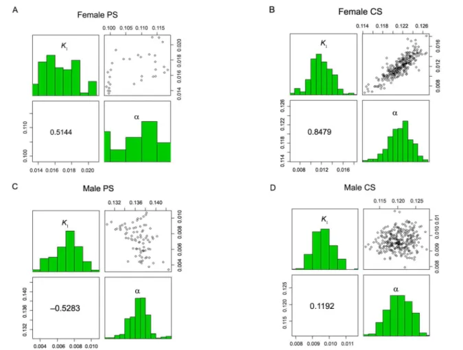
a system in response to multiple variations (climate, gen-otypes, nutritional diet, system, and other factors). The adjusted model for the four specific scenarios ensures greater predictability and can be a useful tool to adapt systems to higher profitability. The negative correlation between the rate constant for addition of DNA and the maintenance requirement energy of animal was found for intact males PS (Figure 2C). This correlation indicates that the animals with faster lean tissue deposition also have better performance because they tend to dilute the energy for maintenance with the greater proportion of energy in-tended for tissue deposition. The joint dispersion matrices of the nonparametric bootstrap estimates, Pearson corre-lation and frequency histograms for k1 and a, are shown in Figures 2A, B, C and D.
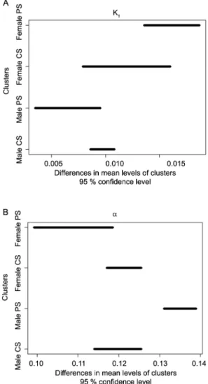
There was no difference between the PS and CS systems within the female gender, considering the pa-rameters k1 and a simultaneously. There was no differ-ence in the CS level change for PS level, regarding the gender factor, in weight gain (k1). This was an expected result, since PS animals have a similar growth rate dur-ing the compensatory gain compared to CS animals (Ta-ble 3). The results show significant differences, about a, between males PS and males CS, with the largest main-tenance of energy average for males PS (Table 3). This behavior in male animals was expected because animals from CS were slaughtered in a shorter time during the feedlot in relation to animals from PS (Table 2).
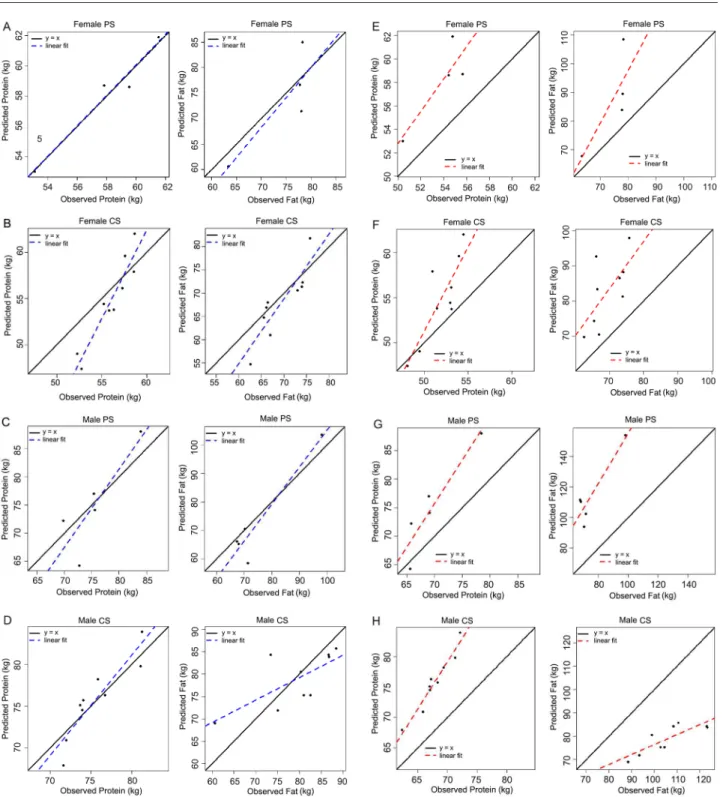
The reparametrized model in this study (Figures 3A, B, C and D) improved predictions of the original parameters (Bos Taurus reference bull, Figures 3E, F, G and H). The bias of the proposed new parameters calculated considering average protein and fat concentration are smaller than the bias considering calculated average predictions of protein and fat concentration using the original calibration of the model by Oltjen et al. (1986), respectively (Table 4). The evaluation of the model (Table 5) using the criteria MSEP, CCC, intercept, slope, AIC, and BIC corroborate the
Table 3 − Descriptive measures, Kolmogorov-Smirnov (KS) normality test (p value) and confidence intervals for the average Davis Growth Model (DGM) parameters with 95 % of confidence.
Gender Previous weaningsystem ConstantsFixed Par. Originalsample Bootstrap p valueKS CI BCPB 3
Mean S.D.8 Lower limit Upper limit
(k2 = 0.0461)
6 k
1 0.0124 0.0167 0.0018 0.0460 0.0136 0.0187
PS4 (k
3 = 0.1430)
6 a 0.1100 0.1082 0.0065 0.0894 0.0993 0.1185
F1 (DNA
max = 308)
7
(k2 = 0.0461)
6 k
1 0.0092 0.0119 0.0020 0.7173 0.0079 0.0160
CS5 (k
3= 0.1430)
6 a 0.1216 0.1214 0.0022 0.9961 0.1171 0.1255
(DNAmax = 308)7 (k2 = 0.0461)
6 k
1 0.0061 0.0067 0.0017 0.1882 0.0035 0.0095
PS4 (k
3 = 0.1430)
6 a 0.1360 0.1374 0.0024 0.1595 0.1311 0.1389
M2 (DNA
max = 462)
7
(k2 = 0.0461)
6 k
1 0.0084 0.0096 0.0005 0.5842 0.0086 0.0108
CS5 (k
3 = 0.1430)
6 a 0.1199 0.1204 0.0031 0.2023 0.1140 0.1255
(DNAmax = 462)7
1Females; 2Males; 3Confidence interval of Biased Corrected Percentile Bootstrap; 4Pasture System; 5Confined System; 6Fixed values based by Oltjen et al. (1986); 7DNA
max was based on direct and linear proportion of mature weight of the breed and gender of these animals;
8Standard Deviation.
Figure 2 − Joint dispersion matrixes of the nonparametric bootstrap estimates, the Pearson correlation, and frequency histograms for k1 and a to the Davis Growth Model A) Female PS (Pasture System); B) Female CS (Confined System); C) Male PS; D) Male CS.
Table 4 − Comparison of average predictions of protein and fat between the new calibrations proposed in this study and calibrations using the original values of Oltjen et al. (1986).
New calibrations1 Original parameters2
Clusters Variables Observed Predicted Bias Predicted Bias
Females Protein (kg d−1) 58.0500 57.9920 0.0579 53.8236 4.2264
PS3 Fat (kg d−1) 74.4000 73.4140 0.9859 87.3991 -12.9991
Females Protein (kg d−1) 54.8777 54.9139 -0.0361 51.9247 2.9669
CS4 Fat (kg d−1) 69.3700 68.8142 0.5635 82.7235 -13.3535
Males Protein (kg d−1) 75.1200 74.4028 0.7171 53.8236 21.2964
PS3 Fat (kg d−1) 75.1000 74.9045 0.1954 87.3991 -12.2991
Males Protein (kg d−1) 75.8111 75.5887 0.2223 67.8307 7.9804
CS4 Fat (kg d−1) 78.9000 79.4407 -0.5407 105.9546 -27.0546
1Parameter fit in the current study; 2Based on parameters (k
1, a) calculated in the Oltjen et al. (2000) study;
3Pasture System; 4Confined System.
results shown in Figures 3A, B, C, D, E, F, G, and H, indicating improvement in performance of the model with new estimates of the current study compared to the original estimates by Oltjen et al. (1986). Therefore, this fitted model was provisionally accepted for growth simulation of Nellore (Bos indicus) and Nellore crossbred animals, although pending further evaluations with an independent dataset.
In this study, k1 and a values were higher than the original DGM parameters (Oltjen et al., 1986). In the study conducted by Oltjen et al. (1986), k1 had a minimum increase of 156 % and the maximum of 389 % compared to the original values (k1 = 0.00429, Table 6), while a had a minimum increase of 126 % and the maximum of 160 % compared to the original values (a
reparameter-Figure 3 − Observed and predicted values for protein and fat. (A – D) modified parameters; (E – H) original parameters (Bos Taurus reference bull); PS: Pasture System; CS: Confined System.
ization of the model with Nellore bulls by Sainz et al. (2006) estimated rates for k1, k3 and a (k1 = 0.00304, k3
= 0.1300, and a = 0.0768), keeping fixed k2 (0.0479) and
DNAmax (462 g). Compared to Sainz et al. (2006), k1 had a minimum increase of 220 % and the maximum of 549 %;
a had a minimum increase of 141 % and the maximum
of 178 % (Table 7). Breeds and genetic improvement are the possible causes of parameter changes.
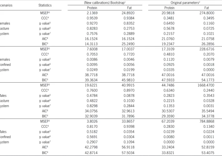
Table 5 − Evaluation of Davis Growth Model (DGM) with the estimates obtained by bootstrap analysis of the current study and evaluation using the original estimates of model Oltjen et al. (1986).
Scenarios Statistics (New calibrations) Bootstrap
1 Original parameters2
Protein Fat Protein Fat
MSEP3 2.1369 24.8920 20.9818 274.8000
CCC4 0.9539 0.9384 0.3481 0.3495
Females p value5 0.9270 0.8352 0.6450 0.1160
Pasture p value6 0.8283 0.2753 0.5678 0.0725
System p value7 0.7576 0.2889 0.2157 0.1021
AIC8 16.1524 16.1524 21.0760 21.0758
BIC9 14.3113 25.2490 19.2347 26.2856
MSEP3 7.6008 17.0037 17.3109 228.6716
CCC4 0.7053 0.7720 0.4810 0.2070
Females p value5 0.0086 0.0046 0.1120 0.0079
Confined p value6 0.0095 0.0056 0.0925 0.0018
System p value7 0.0249 0.0199 0.0335 0.0000
AIC8 38.7718 38.7718 47.0016 47.0016
BIC9 39.3634 45.9810 47.5933 54.1773
MSEP3 19.6221 40.9915 44.7486 1668.4700
CCC4 0.7600 0.8970 0.6340 0.2440
Males p value5 0.4784 0.0878 0.2823 0.3543
Pasture p value6 0.4822 0.1030 0.2215 0.0328
System p value7 0.8298 0.2844 0.1353 0.0031
AIC8 34.0756 32.9613 30.5307 35.5494
BIC9 32.9039 31.7896 29.3590 34.3778
MSEP3 3.8026 33.8657 67.2039 784.8868
CCC4 0.8170 0.9398 0.2830 0.1340
Males p value5 0.5182 0.0354 0.0239 0.0224
Confined p value6 0.5691 0.0304 0.0080 0.0011
System p value7 0.2907 0.1094 0.0000 0.0000
AIC8 42.2798 56.9118 33.2404 52.8159
BIC9 42.8714 57.5034 33.8321 53.4075
1Parameter fit in the current study; 2Based on parameters fit (k
1, a) calculated in the Oltjen et al. (1986) study;
3Mean square error of prediction (smaller is better); 4Concordance Correlation Coefficient (closer to 1 is better); p value5: (H
0: β0 = 0); p value 6: (H
0: β1 = 1); p value 7: (H
0: β0 = 0 and β1 = 1);
8Akaike Information Criterion (smaller is better); 9Bayesian Information Criterion (smaller is better).
Table 6 − Percentage of change of the current values of the parameters in relation to the original values of Oltjen et al. (1986).
Zebu crossbred1 British
(Bos taurus2) Parameter
fit
Females PS3
Females CS4
Males PS3
Males
CS4 Steer
k1 0.0167 0.0119 0.0067 0.0096 0.00429
a 0.1082 0.1214 0.1374 0.1204 0.0860
% of k1 (389 %) k1 (214 %) k1 (156 %) k1 (223 %)
-change a (126 %) a (141 %) a (160 %) a (140 %) -1Parameter fit in the current study; 2Based on parameters (k
1, a) calculated in
the Oltjen et al. (1986) study; 3Pasture System; 4Confined System.
Table 7 − Percentage of change of the current values of the parameters in relation to the original values of Sainz et al. (2006).
Zebu crossbred1 Nellore
(Bos indicus2) Parameter
fit
Females PS3
Females CS4
Males PS3
Males
CS4 Bulls
k1 0.0167 0.0119 0.0067 0.0096 0.00304
a 0.1082 0.1214 0.1374 0.1204 0.0768
% of k1 (549 %)k1 (391 %)k1 (220 %)k1 (315 %)
-change a (141 %)a (158 %)a (178 %)a (156 %) -1Parameter fit in the current study; 2Based on parameters (k
1, a) calculated in
the Sainz et al. (2006) study; 3Pasture System; 4Confined System.
Nellore used by Sainz et al., 2006); and 2) the experiment was conducted with animals from herds selected by Embrapa in 2010, three to seven generations after the Sainz et al. (2006) and Oltjen et al. (1986) studies. These cases reinforce both the improvement through crossing and selection, as well as genetic progress associated with increased k1 and a. In Brazil as in other countries, weight is the main selection criteria with moderate to high genetic
correlation with growth curve parameters (Meyer, 1995; Mignon-Grasteau, 1999), and potentially with k1 and a.
Conclusions
differ from the original values determined by Oltjen et al. (1986). Breeds and genetic improvement are the pos-sible causes of parameter changes. Intact male animals of the pasture system showed negative correlation be-tween the protein deposition rate and requirement for energy maintenance, indicating that the animals with faster lean tissue deposition also have better perfor-mance because they tend to dilute the energy cost for maintenance, with a greater proportion of energy used for tissue deposition. We highlight that the generaliza-tion of this finding demands studies with larger popula-tions. The new estimates of parameter values, instead of the originals, can be used for predictive purposes for crossbred cattle.
Acknowledgements
The authors express their thanks to Coordina-tion for the Improvement of Higher Level Personnel (CAPES) and Brazilian Agricultural Research Corpora-tion (Embrapa) for providing scholarship and Universi-ty of São Paulo/ESALQ academic formation by the first author, the Embrapa Beef Cattle, Animal Nutrition and Growth Laboratory – USP/ESALQ and São Paulo State Foundation for Research Support (FAPESP) for provid-ing the data and grants, as well the Embrapa Eastern Amazon and Embrapa Agricultural Informatics by the scientific partnership group of the Pecus and Animal-Change network.
References
Albertini, T.Z.; Medeiros, S.R.; Torres Júnior, R.A.; Zocchi, S.S.; Oltjen, J.W.; Strathe, A.B.; Lanna, D.P.D. 2012. A methodological approach to estimate the lactation curve and net energy and protein requirements of beef cows using nonlinear mixed-effects modeling. Journal of Animal Science 90: 3867-3878. Bonilha, S.F.M.; Tedeschi, L.O.; Packer, I.U.; Razook, A.G.;
Nardon, R.F.; Figueiredo, L.A.; Alleoni, G.F. 2011. Chemical composition of whole body and carcass of Bos indicus and tropically adapted Bos Taurus breeds. Journal of Animal Science 89: 2859-2866.
Bhowmick, A.R.; Bhattacharya, S. 2014. A new growth curve model for biological growth: some inferential studies on the growth of Cirrhinus mrigala. Mathematical Biosciences 254: 28-41.
Chizzotti, M.L.; Tedeschi, L.O.; Valadares Filho, S.C. 2008. A meta-analysis of energy and protein requirements for maintenance and growth of Nellore cattle. Journal of Animal Science 86: 1588-1597.
Freetly, H.C.; Kuehn, L.A.; Cundiff , L.V. 2011. Growth curves of crossbred cows sired by Hereford, Angus, Belgian Blue, Brahman, Boran, and Tuli bulls, and the fraction of mature body weight and height at puberty. Journal of Animal Science 89: 2373-2379.
France, J.; Gill, M.; Thornley, J.H.M.; England, P. 1987. A model of nutrient utilization and body composition in beef cattle. Animal Production 44: 371-385.
Forni, S.; Piles, M.; Blasco, A.; Varona, L.; Oliveira, H.N.; Lôbo, R.B.; Albuquerque, L.G. 2009. Comparison of different nonlinear functions to describe Nelore cattle growth. Journal of Animal Science 87: 496-506.
Efron, B. 1979. Bootstrap methods: another look at the jackknife. The Annals of Statistics 7: 1-26.
Efron, B. 1981. Nonparametric standard errors and confidence intervals. Canadian Journal of Statistics 9: 139-172.
Hankins, O.G.; Howe, P.E. 1946. Estimation of the Composition of Beef Carcass Cuts. USDA, Washington, DC, USA. (Technical Bulletin, 26.).
Hoch, T.; Agabriel, J. 2004. A mechanistic dynamic model to estimate beef cattle growth and body composition. 1. Model description. Agricultural Systems 81: 1-15.
Marinho, K.N.S.; Freitas, A.R.; Falção, A.J.S.; Dias, F.E.F. 2013. Nonlinear models for fitting growth curves of Nellore cows reared in the Amazon Biome. Revista Brasileira de Zootecnia 42: 645-650.
Marcondes, M.I.; Chizzotti, M.L.; Valadares Filho, S.C.; Gionbelli, M.P.; Paulino, P.V.R.; Paulino, M.F. 2010a. Energy requirements of zebu beef cattle. p. 81-106. In: Valadares Filho, S.C.; Marcondes, M.I.; Chizzotti, M.L.; Paulino, P.V.R., eds. Nutrient requirements of zebu beef cattle BR-CORTE. 2ed. UFV, Viçosa, MG, Brazil.
Marcondes, M.I.; Chizzotti, M.L.; Valadares Filho, S.C.; Gionbelli, M.P.; Paulino, P.V.R.; Paulino, M.F. 2010b. Protein requirements of zebu beef cattle. p. 107-126. In: Valadares Filho, S.C.; Marcondes, M.I.; Chizzotti, M.L.; Paulino, P.V.R., eds. Nutrient requirements of zebu beef cattle BR-CORTE. 2ed. UFV, Viçosa, MG, Brazil.
Meyer, K. 1995. Estimates of genetic parameters for mature weight of Australian beef cows and its relationship to early growth and skeletal measures. Livestock Production Science 44: 125-137.
Mignon-Grasteau, S. 1999. Genetic parameters of growth curve parameters in male and female chickens. British Poultry Science 40: 44-51.
National Research Council [NRC]. 1996. Nutrient Requirements of Beef Cattle. 7ed. The National Academies Press, Washington, DC, USA. p. 234.
Nelder, J.A.; Mead, R. 1965. A simplex algorithm for function minimization. Computer Journal 7: 308-313.
Nesetrilová, H. 2005. Multiphasic growth models for cattle. Czech Journal of Animal Science 8: 347-354.
Oltjen, J.W.; Pleasants, A.B.; Soboleva, T.K.; Oddy, V.H. 2000. Second-generation dynamic cattle growth and composition models. p. 197-209. In: McNamara, J.P.; France, J.; Beever, D.E., eds. Modelling nutrient utilization in farm animals. CAB International, Wallingford, UK.
Oltjen, J.W.; Bywater, A.C.; Baldwin, R.L.; Garrett, W.N. 1986. Development of a dynamic model of beef cattle growth and composition. Journal of Animal Science 62: 86-97.
Press, W.H.; Flannery, B.P.; Teukolsky, S.A.; Vetterling, W.T. 1990. Numerical recipes in C: the art of scientific computing. Cambridge University Press, New York, NY, USA.
Reid, J.T.; Wellington, G.H.; Dunn, H.O. 1955. Some relationships among the major chemical components of the bovine body and their application to nutritional investigations. Journal of Dairy Science 38: 1344-1359.
Sainz, R.D.; Barioni, L.G.; Paulino, P.V.; Valadares Filho, S.C.; Oltjen, J.W. 2006. Growth patterns of Nellore vs British beef cattle breeds assessed using a dynamic, mechanistic model of cattle growth and composition. p. 160-170. In: Kebreab, E.; Dijkstra, J.; Bannink, A.; Gerrits, W.J.J.; France, J., eds. Nutrient digestion and utilization in farm animals: modeling approaches. CAB International, Wallingford, UK.
Soetaert, K.; Petzoldt, T.; Setzer, R.W. 2010. Solving differential equations in R: package deSolve. Journal of Statistical Software 33: 1-25.
Tedeschi, L.O. 2006. Assessment of the adequacy of mathematical models. Agricultural Sciences 89: 225-247.
Tedeschi, L.O.; Fox, D.G.; Guiroy, P.J. 2004. A decision support system to improve individual cattle management. 1. A mechanistic, dynamic model for animal growth. Agricultural Systems 79: 171-204.
Valente, E.E.L.; Paulino, M.F.; Detmann, E.; Valadares Filho, S.C.; Cardenas, J.E.G.; Dias, I.F.T. 2013. Requirement of energy and protein of beef cattle on tropical pasture. Acta Scientiarum 35: 417-424.
Williams, C.B.; Bennett, G.L. 1995. Application of a computer model to predict optimum slaughter end points for different biological types of feeder cattle. Journal of Animal Science 73: 2903-2915.
![Table 1 − Summary descriptive analysis [mean, standard deviation (SD), minimum (Min) and maximum (Max)] of the model input variables for 13 crossbred females.](https://thumb-eu.123doks.com/thumbv2/123dok_br/15861437.662897/2.918.501.846.182.566/summary-descriptive-analysis-standard-deviation-minimum-variables-crossbred.webp)
![Table 2 − Summary descriptive analysis [mean, standard deviation (SD), minimum (Min) and maximum (Max)] of the model input variables for 14 crossbred bulls.](https://thumb-eu.123doks.com/thumbv2/123dok_br/15861437.662897/3.918.69.413.184.560/summary-descriptive-analysis-standard-deviation-minimum-variables-crossbred.webp)