The Brothers Q: multimode entangled photons with parametric down conversion

CONVERSION Stephen Patrick Walborn

Stephen Patrick Walborn

Orientador: Prof. Carlos Henrique Monken

With the last 10 years of life spread (smeared might be a better word) over two coast lines and two continents, I look back and realize that the reason I am where I am is due to the friendship and support of countless individuals. As I look back, the quantity of people seems overwhelming. Here I go:

I cannot offer enough thanks to my advisor Carlos Henrique Monken for his guid-ance, advice, and friendship over the last 6 years. I am grateful also for his dedication to his students and his patience in general, and especially with my portuguese.

This work was performed with financial support from the brasilian funding agency Conselho Nacional de Desenvolvimento Cient´ıfico e Tecnol´ogico (CNPq); Thank you.

The past few years in the laboratory have been enjoyable and productive mostly thanks to fellow lab rats Wallon A. T. Nogueira and ´Alvaro N. de Oliveira. Thank you for always being available to discuss and distract.

I would like to thank Professors Marcelo O. Terra Cunha, Sebasti˜ao de P´adua, Paulo Henrique Souto Ribeiro and Reinaldo Viana, as well as Dilson P. Caetano for valuable conversations over the last few years. Thanks also to everyone in Sebasti˜ao’s lab for discussions and frequent equipment loans.

I thank Professors Johnny Powell and Osiel Bonfim for their support and encour-agement.

The past 6 years in Belo Horizonte would not have been fun (or even possible) without the many friends that I have made here. Thanks go out to:

The inhabitants of the Lama Lar (na minha casa todo mundo ´e lama. . .): Nathan, Cabelim, ´Alvarot (. . . like a crazed Leati. . .), Alex; also Bira, M´arcio, M´ario, Aline, Alexandre, Mˆonica, Erlinda, Erildo, Cristiano, Tatiana, Simone, Craud˜ao, Rosˆangela, Terra, Ana Mara, Dona Ad´elia and Seu Ign´acio, Catarina, Expedito, Lucas, Luciana, and everyone in the physics dept.

Thank you Marluce for the laughter and the constant supply of official letters and documents which kept me in check with the feds;

Thanks to the physics department staff, especially Seu Jo˜ao Batista and everyone

times, and for not disowning me for my late email responses and other correspondence misdemeanors. Thank you Katie, Todd, Matt, Kevin, Eric, southern Mark, Chuck and Betsy, Doc, Sarah B, Mark, Amanda Hugenkeis, Luca James, Bret, Natasha, Seth, Brahmani, Alex, Ovide, Chad, Ren´e, Matei, my grandparents, aunts, uncles and cousins, and everyone else you know who you are.

Thank you Celeste.

Thank you dad and Kathy.

RESUMO xv

ABSTRACT xvii

Author’s Note xix

1 Introduction 1

1.1 Background . . . 1

1.2 Quantum Information . . . 2

1.2.1 The qubit . . . 3

1.3 Motivation . . . 4

1.3.1 Spontaneous Parametric Down-conversion . . . 5

1.4 Objectives . . . 7

1.4.1 Publications . . . 8

2 Fundamentals 9 2.1 Spontaneous parametric down-conversion . . . 9

2.1.1 Introduction . . . 9

2.2 Quantum theory of SPDC . . . 10

2.2.1 Quantum theory of SPDC . . . 11

2.2.2 The Fresnel and paraxial approximations . . . 15

2.2.3 The angular spectrum . . . 16

2.2.4 The biphoton state . . . 17

2.2.5 The biphoton wavefunction . . . 18

2.2.6 The coincidence count rate . . . 19

2.3 Engineering entanglement . . . 19

2.3.1 Polarization entanglement with SPDC. . . 20

2.3.2 Discriminating polarization-entangled Bell-states . . . 22

2.3.3 Momentum entanglement with SPDC . . . 25

2.4.2 Modifying the laser cavity . . . 27

2.4.3 Laguerre-Gaussian modes . . . 28

2.4.4 Mode-conversion . . . 28

3 Multimode Hong-Ou-Mandel interference 33 3.1 Introduction . . . 33

3.2 Multimode Hong-Ou-Mandel interference . . . 34

3.2.1 Two-port coincidence detection . . . 35

3.2.2 Same-port coincidence detection . . . 37

3.2.3 Analysis . . . 38

3.3 Experiment and results. . . 41

3.4 Conclusion . . . 44

4 Optical Bell-state analysis 45 4.1 Optical Bell-state analysis . . . 45

4.2 Bell-state analysis using multimode HOM interference . . . 48

4.2.1 Theory . . . 48

4.2.2 Experiment and results. . . 50

4.3 Complete Bell-state analysis in the coincidence basis . . . 53

4.4 Hyperentanglement-assisted Bell-state analysis . . . 54

4.4.1 Introduction . . . 54

4.4.2 Hyperentanglement . . . 54

4.4.3 Bell-state analysis . . . 56

4.4.4 Applications . . . 60

4.5 Conclusion . . . 62

5 Conservation and Entanglement of Orbital Angular Momentum in SPDC 65 5.1 Introduction . . . 65

5.2 Theory . . . 67

5.2.1 The state generated by SPDC . . . 67

5.2.2 Biphoton phase measurements. . . 71

5.3 Experiment and results. . . 72

5.4 Conclusion . . . 76

6 Generation of Entangled Hermite-Gaussian modes with SPDC 79 6.1 Introduction . . . 80

6.2 Conservation of Hermite-Gaussian modes with SPDC . . . 80

6.3 Entanglement of Hermite-Gaussian modes . . . 87

6.3.1 Finite dimension . . . 89

6.3.2 Infinite dimension . . . 93

6.3.5 Hyperentangled states . . . 99 6.4 Conclusion . . . 99

7 Conclusion 101

7.1 Conclusion . . . 101

A Derivation of the coefficients Cnm

jkut 105

A.1 Derivation of the coefficients Cnm

jkut . . . 105

B Maple Programs 109

B.1 Maple program to calculate coefficientsCnm

jkut . . . 109

B.2 Maple program to calculatetrρ2 _{for0≤ N ≤5 . . . . 112} B.3 Maple program to calculatetrρ2 _{for0≤ R ≤5 . . . . 115}

Bibliography 117

2.1 Diagram of type-II spontaneous parametric down-conversion . . . 11

2.2 Experimental setup for generating and testing Bell-states. . . 21

2.3 Results of polarization analysis of Bell-states . . . 23

2.4 Cartoon of an ideal Bell-state analyzer. . . 24

2.5 Optical Bell-state analyzer. . . 24

2.6 Sources of momentum-entangled photons . . . 25

2.7 Diagram of a transverse mode converter . . . 28

2.8 Digital photographs of transverse modes produced in the laboratory . . . . 31

3.1 Multimode Hong-Ou-Mandel Interferometer. . . 34

3.2 Experimental setup for multimode HOM interference . . . 40

3.3 Experimental results of multimode HOM interference for a symmetric po-larization state . . . 42

3.4 Experimental results of multimode HOM interference for theψ−_polarization state . . . 43

3.5 Experimental results of multimode HOM interference for a symmetric po-larization state and pump beam of undefined parity . . . 43

4.1 Incomplete Bell-state analyzer . . . 47

4.2 Experimental setup for optical Bell-state analysis . . . 50

4.3 Two-photon interference for _|ψ+_{i, |ψ}−_{i and |φi polarization states with} hg_{01 pump beam . . . . 51}

4.4 Experimental results for incomplete Bell- state measurement . . . 52

4.5 Kwiat and Weinfurter’s complete Bell-state analyzer using hyperentangled states . . . 52

4.6 SPDC source of hyperentangled photons . . . 54

4.7 The hyperentangled Bell-state analyzer . . . 56

4.8 The hyperentangled Bell-state analyzer for momentum Bell-states . . . 59

5.1 Experimental setup to show conservation of orbital angular momentum . . 72

6.1 Diagram of entangled HG mode generation . . . 82 6.2 Total probability of HG mode generation as a function of the total order

j+k+u+t. . . 84 6.3 CoefficientsCnm

jkutfor ahg00andhg11pump beam with widthwp = 0.1mm

up to order _O= 4.. . . 86 6.4 Total probability of HG mode generation as a function of the orderj+k+

u+t showing normalization . . . 87 6.5 trρ2 _{for0≤ N ≤5 forhg}

00, hg01, hg11 and hg02 pump beams. . . 94 6.6 trρ2 _{for0≤ R ≤5 forhg}

00, hg01,hg11 and hg02 pump beams. . . 95 6.7 Possible experimental setup to generate arbitrary two-photon states with

first-order HG modes. . . 97

3.1 Summary of two-photon multimode interference dependence . . . 40

4.1 Summary of detector signatures for incomplete Bell state analysis . . . 49

4.2 Detector signatures for polarization Bell-state analysis using the momentum state_|ψ+_{i as an ancilla. . . . . 58}

4.3 Detector signatures for momentum Bell-states using the polarization state |Ψ+_{i as an ancilla . . . . 59}

6.1 Amplitudes and probabilities for gaussian pump beam . . . 85

6.2 Amplitudes and probability for hg₁₁ pump beam . . . 88

Esta tese ´e um estudo das propriedades quˆanticas de f´otons multimodais gera-dos por meio da convers˜ao param´etrica descendente espontˆanea, tendo por objetivo a aplica¸c˜ao em problemas de informa¸c˜ao quˆantica, tais como medidas de estados de Bell e a gera¸c˜ao de f´otons emaranhados nos graus de liberdade espaciais transversais.

Como uma primeira investiga¸c˜ao, realizamos um estudo te´orico sobre a ferˆencia Hong-Ou-Mandel (HOM) multimodal. Mostramos que os efeitos de inter-ferˆencia de quarta ordem dependem das propriedades transversais do estado do bif´oton (par de f´otons). Devido `a transferˆencia do espectro angular do feixe bombeador para este estado, mostrado por Monken et al. [Phys. Rev. A, 57 3123 (1998)], a paridade do feixe bombeador pode ser usada como um parˆametro de controle da interferˆencia de quarta ordem. Executamos uma experiˆencia de interferˆencia HOM usando feixes Hermite-Gaussianos de primeira ordem como feixe bombeador. Os resultados experi-mentais mostram que o comportamento da interferˆencia de quarta ordem depende da paridade do feixe bombeador, como foi previsto teoricamente.

Uma primeira aplica¸c˜ao da interferˆencia HOM multimodal pode ser feita na an´alise de estados de Bell, que utiliza interferˆencia de quarta ordem. As t´ecnicas precedentes requerem detectores que sejam sens´ıveis ao n´umero de f´otons. Por outro lado, com interferˆencia HOM multimodal esta an´alise pode ser feita usando detectores de um f´oton. Para mostrar que a interferˆencia multimodal poderia ser usada para melhorar estes m´etodos, realizamos uma experiˆencia simples de discrimina¸c˜ao dos es-tados de Bell usando f´otons multimodais emaranhados em polariza¸c˜ao. Trˆes grupos de estados de Bell foram identificados na base de coincidˆencias (com detectores de um f´oton). Al´em disto, discutimos dois m´etodos similares para an´alise de estado de Bell utilizando estados hiperemaranhados (emaranhados em mais de um grau de liber-dade). Mostramos que uma proposta precedente de Kwiat et al. [Phys. Rev. A 58 R2623 (1998)], que requer f´otons emaranhados em mais de um grau de liberdade, fun-cionar´a melhor usando a interferˆencia HOM multimodal. Finalmente, propomos um novo m´etodo de an´alise de estados de Bell de f´otons hiperemaranhados que n˜ao requer

dos pela convers˜ao param´etrica descendente, investigamos a conserva¸c˜ao e emaran-hamento de momento angular orbital neste processo. Sabe-se bem que um campo eletromagn´etico pode carregar momento angular orbital na forma de uma fase azimu-tal no plano transversal. Desta forma, mostramos teoricamente que a gera¸c˜ao de f´otons emaranhados em momento angular orbital na convers˜ao param´etrica descendente pode ser explicada atrav´es da transferˆencia do espectro angular. Realizamos uma experiˆencia multimodal simples de interferˆencia de quarta ordem que comprovou as nossas previs˜oes te´oricas.

Finalmente, estudamos a gera¸c˜ao de f´otons emaranhados nos modos transversais Hermite-Guassianos. Usando a teoria da transferˆencia do espectro angular, mostramos que a convers˜ao param´etrica descendente gera pares de f´otons emaranhados em mo-dos Hermite-Gaussianos, e para quaisquer pares destes momo-dos, calculamos a ampli-tude de gera¸c˜ao. Al´em disto, discutimos a gera¸c˜ao de estados maximamente e n˜ao-maximamente emaranhados usando modos de primeira ordem.

This thesis is a study of the quantum properties of multimode entangled photons created by spontaneous parametric down-conversion. More specifically, we attempt to utilize this multimode character in quantum information tasks such as Bell-state measurement and the generation of photons entangled in transverse spatial degrees of freedom.

As a first investigation, a theoretical study of multimode Hong-Ou-Mandel inter-ference was conducted. It is shown that the fourth-order interinter-ference effects depend upon the transverse spatial properties of the biphoton. Due to the transfer of the angu-lar spectrum of the pump beam to the biphoton state shown by Monken et al. [Phys. Rev. A 57 3123 (1998)], the parity of the pump beam can be used as a control pa-rameter of fourth-order interference. A Hong-Ou-Mandel interference experiment was performed using first-order Hermite-Gaussian pump beams. The experimental results show that the observed fourth-order interference behavior depends upon the parity of the pump beam.

down-conversion. It is well known that a light field can carry orbital angular mo-mentum in the form of an azimuthal phase dependence. We show theoretically that the angular spectrum transfer enables the generation of photons entangled in orbital angular momentum. A simple multimode fourth-order interference experiment was performed which confirms these theoretical predictions.

Finally, we studied the generation of photons entangled in Hermite-Gaussian modes. Using the theory of angular spectrum transfer, we show that spontaneous parametric down-conversion generates photons entangled in Hermite-Gaussian modes and calculate the probability amplitude to generate arbitrary Hermite-Gaussian modes. In addition we discuss the generation of maximally entangled Bell-states and arbitrary bipartite pure states.

This document was compiled with LA_{TEX using the hyperref package, which}

pro-vides the PDF file with inter-document links for all cited references, sections, figures, tables and equations, as well as links to URLs. Text appearing in dark blue indicates a link to a reference within the document, while text appearing in red indicates a link to an internet URLs. The backref option has been used, which, for each reference in the bibliography, provides a link to the section(s) in which that reference was cited. The links should work with most PDF viewers, including Adobe Acrobat Reader and Apple Preview.

1

Introduction

1.1

Background

In1964_{, John Bell showed that entanglement can be stronger than strictly} classi-cal correlations. That is, he showed that the predictions of quantum mechanics conflict with those of any local hidden variable theory, the sort suggested by EPR. Through a simple argument, Bell derived an inequality that any local realistic probability theory must obey. Violation of Bell’s inequality implies that once realism is assumed, quantum mechanics is inherently non-local. However, it has been shown that there is no danger of violating relativity, since information cannot be sent through quantum correlations alone [4] 1_{. Later, Clauser, Horne, Shimony and Holt [5] reformulated Bell’s inequality} to fit actual experimental situations. This set the stage for a multitude of experiments testing Bell’s inequality [6, 7, 8, 9, 10, 11, 12, 13, 14, 15, 16, 17, 18, 19]. Nearly all experimental results have agreed with quantum mechanics, though none has been en-tirely conclusive due to various technical loopholes. A few skeptics notwithstanding, most scientists are placing their money on quantum theory.

1.2

Quantum Information

Ironically, what was first seen as a serious flaw in quantum theory has since led to a lot of interesting new physics as well as promising technical applications. Specifically, it has been shown that it may be advantageous to use quantum systems to process and communicate information. Paul Benioff [20], David Deutsch [21, 22], Richard Feynman [23,24] and others laid some of the first bricks in the theoretical foundations of quantum computation. Benioff and Deutsch developed the idea of the Quantum Turing Machine, a theoretical quantum computer, and Feynman pointed out that efficient simulation of a quantum system can only really be performed by another quantum system. Deutsch formulated the first quantum algorithm with a speed-up over its classical counterpart [22], and roughly ten years later, Peter Shor provided an algorithm that showed that a quantum computer could be used to factor large numbers faster than any known classical computer algorithm [25, 26]. This caught the attention of the non-physics community, since the difficulty of factorization plays a key role in many cryptography schemes, including the RSA protocol, which is widely used to send encrypted information such as credit card numbers for on-line internet purchases. Cryptographers and internet shoppers need not worry, however. Several cryptography

1

protocols, such as the one-time pad for example, are known to be secure provided that two users can establish a secret random key string. In 1984_{, Gilles Brassard} and Charles Bennett [27, 28], and later Artur Ekert [29] showed that the laws of quantum physics guarantee secure communication with quantum key distribution. In fact, cryptography based on quantum key distribution is the only encryption scheme that has been proven to be secure, provided the encryption scheme functions within certain thresholds. Since the early 1990_{’s many sub-fields have developed, including} quantum key distribution and quantum cryptography, quantum dense coding, quantum communication and quantum computation. All of these fields, and others, now form the field of Quantum Information [30].

1.2.1 The qubit

In contrast with the classical binary “bit”, the basic unit of quantum information is known as the qubit. Whereas the bit can be found in the logical states 0 or 1, the quantum bit is a two-state quantum system that can be found in the arbitrary superposition α_|0_i+β_|1_i. The only restriction placed on the complex coefficients α and β is that they obey the normalization condition _|α_|2_+|β|2 _{= 1. Many two-level}

quantum systems, such as photon polarization, can represent a qubit. The quantum states |0i and |1i correspond to the classical logic states 0 and 1, and are known as the computational basis. The fact that quantum states can be superpositions of the computational basis states gives rise to a quantum parallelism that is not available in ordinary (digital) classical computation. Furthermore, quantum superposition is at the heart of quantum entanglement, which is now regarded as a physical resource to be used in computation and communication tasks. For example, to entangle two qubits all that is required is quantum superposition and a classical two-bit logic operation such as a cnot _{gate [30].}

As evidence of the importance (or at least the recent popularity) of the qubit, I give you:

quantum bit n. The smallest unit of information in a computer designed to manipulate or store information through effects predicted by quantum physics. Unlike bits in classical systems, a quantum bit has more than two possible states: a state labeled 0, a state labeled 1, and a combination of the two states that obeys the superposition principle.

-The American Heritager _{Dictionary of the English Language, Fourth Edition}

Copyright c 2000 by Houghton Mifflin Company.

As to the history and appropriateness of the word itself:

“Qubit seems to have been used first in print by Benjamin Schumacher, ‘Quan-tum coding,’ Phys. Rev. A 51, 2738-2747 (1995). A brief history of the term can be found in the Acknowledgments of this paper. Although qubit honors the English rule that q should be followed by u, it ignores the equally powerful re-quirement that qu should be followed by a vowel. My guess is that it has gained acceptance because it visually resembles an ancient English unit of distance, the homonymic cubit. To see its ungainliness with fresh eyes, imagine that Dirac had written qunumber instead of q-number, or that one erased transparencies and cleaned ones ears with Qutips.”

-N. David Mermin, “From Cbits to Qbits: Teaching computer scientists quantum

mechanics”, American Journal of Physics, 7123 (2003), footnote 3.

1.3

Motivation

Evidently, the ability to produce and control entangled quantum systems has tremen-dous advantages. In addition to the possible technological applications, the exper-imental study of entanglement has shed much light on the foundations of quantum mechanics. There are several physical systems that have played a large role in re-cent investigations, including Nuclear Magnetic Resonance, Cavity QED, Solid-State devices, and optical systems.

Given the relative ease with which one can create and send entangled photons from one place to another, optical systems are the leading contenders for implemeta-tions of quantum cryptography and long-distance quantum communication. Quantum cryptographic systems are well within the limits of contemporary technology. Plug and play quantum cryptography devices using fiber optics have been developed, and recent experiments have been performed using laser beams propagating in free space during daylight hours [31].

elements such as wave plates, beam splitters and phase shifters. However, controlled gates acting on multiple photons remain difficult due to the nonlinear interaction re-quired. Recently, Knill, Laflamme and Milburn have shown that scalable quantum optical computation is possible using only linear optical elements [33]. Several quan-tum optical controlled logical gates have been proposed [33, 34, 35, 36], which rely on two-photon interference at a beam splitter, with photodetection and post-selection providing the non-linearity [33]. Andrew White’s group has recently built [37] the linear-optical cnot _{gate proposed in [35]. A current drawback to these gates is the} low reliability and low efficiency, mostly due to detector inefficiency [38].

There is also the possibility of encoding information in more than one degree of freedom of the photon, resulting in 2 or more qubits per photon. Logic gates and quantum algorithms have been performed using polarization and spatial modes of the same photon [39]. Our group has developed a universal quantum cnot _{gate, which} acts on the polarization and the first-order Hermite-Gaussian transverse spatial mode of the same photon [40, 41]. Recently and independently, Fiorentino and Wong have built an improved device and demonstrated it’s operation at the single photon level [42].

1.3.1 Spontaneous Parametric Down-conversion

One of the most important resources in testing the foundations of quantum mechan-ics as well as quantum information protocols are entangled photons produced using spontaneous parametric down-conversion (SPDC). SPDC was first studied theoreti-cally by Klyshko [43] in 1969 _{and experimentally by Burnham and Weinberg [44] in} 1970_{. Since then, there have been many studies investigating the various non-classical}

properties exhibited by the down-converted “twin” photons.

In SPDC, a pump photon excites a nonlinear crystal, creating two daughter photons. There are several physical constraints that can give rise to entanglement: energy conservation, momentum conservation and phase matching. These constraints will be discussed in more detail in section 2.1. Taking advantage of these constraints, physicists have been able to generate photons that are entangled in polarization [13,16], linear momentum [10], energy [11] and orbital angular momentum [45, 46, 19]. Many experiments have been performed using SPDC, including:

• quantum erasers [47, 48, 49, 50, 51]

• quantum dense coding [52]

• quantum key distribution [53, 54, 55]

• quantum teleportation [56,57, 58]

• entanglement swapping [59]

• quantum “cloning” [60, 61]

• quantum logic gates [36,37]

• entanglement distillation/concentration/purification [62, 63]

• two-photon interference effects [64, 65, 66,67, 68]

• spatial antibunching [69,70]

and others. A terrific reference for theoretical and experimental work is Ad´an Cabello’s Bibliographic guide to the foundations of quantum mechanics and quantum information, (quant-ph/0012089) avalaible on the Los Alamos eprint server (http://arxiv.org), which is updated several times a year.

1.4

Objectives

During this doctoral research, several experiments and theoretical investigations were conducted. The main objective and central theme was to use the theory of transfer of angular spectrum in quantum information tasks. The main topics present are multi-mode interference, Bell-state analysis and generation of entangled states with SPDC.

Multimode interference. We have performed several experiments investigating two-photon interference with a variety of pump beams with different transverse spatial properties. We have discovered that the transverse profile of the pump beam can be used to control two-photon interference of down-converted photon pairs. The theory and experiment are presented in chapter 3.

Optical Bell-state analysis. This additional control parameter provided by multi-mode interference is useful in performing aBell-state measurement, that is, distinguish-ing between the four Bell-states. The entangled Bell-states and Bell-state measurement are essential to many quantum information schemes, including quantum dense coding and quantum teleportation. In chapter 4, we present experimental results for an im-proved Bell-state measurement scheme using multimode two-photon interference as well as theoretical results for hyperentangled Bell-state analysis.

Generating entangled states. Exploring the possibility of entanglement in other de-grees of freedom is a potentially fruitful line of research. It has been demonstrated that orbital angular momentum is conserved in SPDC [45, 46, 82], and Bell’s inequality-type experiments have been performed [19], showing that the down-converted photons are entangled in orbital angular momentum. In chapter 5 theoretical results are pre-sented which show that the two-photon state generated by SPDC is indeed entangled in orbital angular momentum. To prove the validity of our theoretical results, we investi-gate the amplitude and phase characteristics of the two-photon state using multimode interference.

in Hermite-Gaussian modes.

1.4.1 Publications

Below is a list of journal articles that have been either published or submitted to be published during this doctorate research. Items marked with an asterisk are related to topics covered in this thesis but are not explicitly discussed.

1. S. P. Walborn, A. de Oliveira, S. P´adua and C. H. Monken, “Multimode Hong-Ou-Mandel Interference”, Physical Review Letters 90, 143601 (2003).

2. S. P. Walborn, W. A. T. Nogueira, S. P´adua and C. H. Monken, “Optical Bell-state analysis in the coincidence basis”, Europhysics Letters 62, 161-167 (2003).

3. S. P. Walborn, S. P´adua and C. H. Monken, “Hyperentanglement-assisted Bell-state analysis”, Physical Review A 68, 042313 (2003).

4. ∗ W. A. T. Nogueira, S. P. Walborn, S. P´adua and C. H. Monken, “Generation of a Two-Photon Singlet Beam”, Physical Review Letters 92, 043602 (2004). 2 5. S. P. Walborn, R. S. Thebaldi, A. de Oliveira, S. P´adua and C. H. Monken,

“Conservation and entanglement of orbital angular momentum in parametric down-conversion”, Physical Review A 69, 023811 (2004).

6. S. P. Walborn, S. P´adua and C. H. Monken, “Conservation and entanglement of Hermite-Gaussian modes in parametric down-conversion”, accepted for publica-tion in Physical Review A, (2005).

7. S. P. Walborn, W. A. T. Nogueira, A. N. de Oliveira, S. P´adua and C. H. Monken, “Multimode Hong-Ou-Mandel Interferometry”, Brief Review to be published in Modern Physics Letters B, (2005).

2

2

Fundamentals

In this chapter, the fundamental theoretical results and experimental techniques

used in this work are introduced.

2.1

Spontaneous parametric down-conversion

Spontaneous parametric down-conversion (SPDC) [43,44] is a nonlinear optical process in which a pump beam photon with wave vector kp and frequency ωp propagating inside a nonlinear optical medium is spontaneously converted into two photons, with wavevectors ks, ki and frequencies ωs,ωi, respectively. Here pstands for “pump” and s and i refer to the down-converted fields1_{. Under most circumstances, the quantum} state of the two down-converted photons is non-separable, meaning that it cannot be written as a product of two one-photon states. Thus the two-photon, or biphoton state must be regarded as a single entity, which results in a plethora of interesting quantum phenomena. This non-separability arises from the various constraints and conservation laws present in the SPDC process.

As we will see in the next section, energy is nearly conserved in SPDC, so that

ωp =ωs+ωi. (2.1)

1

If the nonlinear crystal is thin (on the order of a few millimeters), the transverse component of momentum is nearly conserved, giving

q_p =q_s+q_i. (2.2)

In order to satisfy the conservation of momentum inside the uniaxial birefringent crys-tal, there are certain phase-matching conditions [83] to be satisfied. In a uniaxial crystal, there are two ways of satisfying the phase matching condition, known as type I and type II. In type I phase matching, a pump photon polarized in the extraordinary (e) direction creates two ordinarily (o) polarized photons:

e−→oo type−I (2.3)

whereas in type-II, the down-converted photons are orthogonal:

e −→eo or o−→eo type−II (2.4)

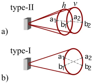
The down-converted light is emitted in a solid cone or cones (depending on the type of phase matching) with its point(s) in the center of the crystal. For type-I, light of a given wavelength is emitted around the rim of a single cone. The cones corresponding to different wavelengths are all coaxial. Photon pairs are emitted on opposite sides of the cones.

The situation is slightly more complicated for type-II, in which there are two cones for each wavelength, as shown in figure 2.1. Down-converted light that is extraordi-narily polarized is emitted on one cone, while ordiextraordi-narily polarized light is emitted on the other cone. The extraordinary cones corresponding to different wavelengths are coaxial, as are the ordinary cones.

2.2

Quantum theory of SPDC

birefringent non-linear crystal

o polarization

laser beam

e polarization

TRANSVERSE PLANE

o e

712 nm 702 nm 692 nm

Figure 2.1: Type-II spontaneous parametric down-conversion. The inset shows the arrange-ment of the cones of light in the transverse plane for 3 different wavelengths in a negative uniaxial crystal. Note that, due to the phase matching conditions, larger (smaller) wavelengths result in a larger cone for extraordinary (ordinary) polarization. The triangles, circles and squares give examples of regions where photon pairs can be found.

2.2.1 Quantum theory of SPDC

When a sufficiently weak electric field E propagates through a second-order nonlinear optical medium, the electrical polarization of the medium is given by [87, 88]

P(r, t) =ǫ0

∞ Z

0

χ(1)(t′)E(r, t₋t′)dt′

+ ∞ Z

0

∞ Z

0

χ(2)(t′, t′′)E(r, t₋t′)E(r, t₋t′′)dt′dt′′. (2.5)

We begin by defining a Hamiltonian

H=_H0+HI, (2.6)

where _H0 is the linear component given by

H0 =

1 2

Z

V

and the “perturbation” HI is the nonlinear component, given by

HI = 1 2

Z

V

E_·P_nl

=1 2

Z

V

∞ Z

0

∞ Z

0

χ(2)_ijk(t′, t′′)Ei(r, t)Ej(r, t−t′)Ek(r, t−t′′)drdt′dt′′, (2.8)

where Pnl is the nonlinear component of the polarization. From this point on we

concern ourselves only with this nonlinear portion.

The electric field can be expanded in terms of plane waves:

E(r, t) = E+(r, t) +E−(r, t), (2.9)

with

E+(r, t) = √1

V X

k,s

ek,sεkαk,se

i(k·r−ωt) ₌

E−(r, t)∗

(2.10)

and εk=

p

~_{ω(k,s)/2ǫV, where}

- ǫ0 ≡ free space permittivity

- V_≡crystal volume

- k_≡ wavevector inside crystal

- s_≡ polarization

- ek,s ≡ two-dimensional polarization vector

- ω _≡ frequency.

We adopt the usual method of quantization of the electric field, letting αk,s −→ ak,s,

where ak,s is the photon destruction operator. Then, the electric field becomes a field

operator, given by

E+(r, t)_−→E+(r, t) = √1

V X

k,s

ek,sεkak,se

i(k·r−ωt) ₌

E−(r, t)†

Substituting expression (2.11) into the classical Hamiltonian (2.8) we have a quantum Hamiltonian operator

HI = 1 2V3/2

X

ks,s_s

X

ki,s_i

X

kp,s_p

f∗(ωs)f∗(ωi)f(ωp)a†_ks,s_sa

†

ki,s_iakp,sp×

ei(ωs+ωi−ωp)t_[χijk(e

ks,s_s)

∗

i(eki,s_i)

∗

j(ekp,s_p)k]

Z

V

e−i(ks+ki−kp)·r_dr

+h.c._{, (2.12)}

where

f(ωj) = i s

~_ω(kj,sj)

2ǫon(kj,sj)2

. (2.13)

Here n(k_j,sj) is the index of refraction of the nonlinear medium. We have also elimi-nated all terms which do not conserve energy and have defined

χijk _≡χ(2)_ijk(wp =ωs+ωi) +χ(2)_ijk(w2 =ωs+ωp) +χ(2)_ijk(ws =ωi+ωp) (2.14)

with

χ(2)_ijk(ω =ω′+ω′′) = ∞ Z 0 ∞ Z 0

χ(2)_ijk(t′, t′′)e−i(ω′_t′_+ω′′_t′′₎

drdt′dt′′. (2.15)

Hereh.c._{denotes the Hermitian conjugate. To find the quantum state at a given time} t, we assume that the nonlinear interaction is turned on at timet−t1 when the system

is in the initial state |ψ(t−t1)i. When the interaction time t1 is much longer than

the coherence times of the down-converted fields and the pump field, a steady state is reached2_:

|ψ(t)_i=U(t, t₋t1)|ψ(t−t1)i (2.16)

where

U(t, t₋t1) = exp

  1 i~ t Z

t−t1

dτHI(τ) 

. (2.17)

If the pump field is sufficiently weak, such that the interaction time is small compared to the average time between down-conversions, then we can Taylor expand and keep only the two-photon term:

U(t, t₋t1) = 1 +

  1 i~ t Z

t−t1

dτHI(τ) 

+· · · . (2.18)

2

It is straighforward to show that

Z t

t−t1

HI(τ)dτ = 1 2V3/2

X

ks,s_s

X

ki,s_i

X

kp,s_p

f∗(ωs)f∗(ωi)f(ωp)a†ks,s_sa

†

ki,s_iakp,sp×

ei(ωs+ωi−ωp)(t−t1/2)_[χijk(e

ks,s_s)∗_i(ek_i,s_i)∗_j(ek_p,s_p)k]×

sinc((ωs+ωi₋ωp)t1/2)

Z

V

e−i(ks+ki−kp)·r_dr

+h.c. _(2.19)

The conservation of energy restriction is contained in the sinc _≡ (sinx)/x function. For sufficiently larget1, only terms withωs+ωi ≈ωp will contribute substantially, and

we can approximate the sinc function by a delta function. Integration in r leads to a similar sinc function involving the wavevectors, which provides the conservation of momentum condition.

In calculating the two-photon state of the down-converted photons, there are two basic approximations that can be made: the monomode approximation and the monochromatic approximation. These approximations facilitate not only the

calcula-tions but also the recognition of any interesting physics that may be present. The monomode approximation considers the fact that experiments are usually performed using narrow detection apertures which define the propagation direction of the down-converted photons. The monochromatic approximation recognizes that most experi-ments are realized using narrow interference filters, determining the magnitude of the wave vectors. Most treatments use at least one of these approximations.

Utilized in the majority of the work of the quantum optics group at UFMG [77,89], the quantum theory of SPDC under the monochromatic approximation enables one to consider multimode (multi-directional) situations. This enables the study of transverse spatial characteristics of the biphoton. Our calculation of the quantum state of the biphoton will use the following assumptions and/or approximations:

1. The monochromatic approximation is valid for the down-converted photons, which are detected using narrow band interference filters.

3. Photons in the pump beam can be accurately represented by a coherent state.

4. We will work in the paraxial approximation around different axes zp, zs and zi for the pump and down converted photons, respectively.

2.2.2 The Fresnel and paraxial approximations

Let us assume that an optical field is propagating along the z direction. Here we are considering only monochromatic waves with k=_|k_|constant, such that for each wave vector k= (q, kz) with k2 _=q2_+k2

z, we can solve for the kz component:

kz =pk2_−q2 _≈k

1₋ q

2

2k2

, if q2 _≪k2. (2.20)

The above approximation, known as the Fresnel approximation, is obtained by simple Taylor expansion and is valid when q2 _{≪ k}2_{. To see the robust validity of the Fresnel}

(paraxial) approximation, let us set q=k/2 and perform the simple calculation:

k

1− q

2

2k2

= 7

8k, while the exact form gives:

p

k2_−q2 ₌

√

3 2 k ≈

6.928 8 k.

Even for a huge value of q, the Fresnel (paraxial) approximation gives an error of only about 0.01. In the experiments considered in this thesisq ∼k/100, which corresponds to an error less than 0.00001.

The Fresnel approximation is essentially a particular application of the more general paraxial approximation. In geometric optics, where light is represented by rays, paraxial rays are those that lie at small angles to the optical axis of the optical system under consideration. If we were to draw rays from the origin to points k in k-space satisfying the approximation in expression (2.20), they would be paraxial rays. In this respect the paraxial approximation and the Fresnel approximation are essentially the same. Throughout this thesis we will make use of both the Fresnel and paraxial approximations, though starting in the next section we will refer to both as the paraxial approximation.

wavefront normals are paraxial rays. In wave optics an optical wave E(r, t) satisfies the wave equation:

∇2_{E(r, t)−} 1

c2

∂2

∂t2E(r, t) = 0.

If one considers that the optical wave is monochromatic with harmonic time depen-dence, so that E(r, t) = _E(r) exp(iωt), where ω is the angular frequency, one arrives at the Helmholtz equation:

∇2E(r) +k2_E(r) = 0.

If we now consider only paraxial waves propagating near the z axis, we can write

E(r) = U(r) exp(ikz), where U(r) is a slowly varying function of r such that E(r) maintains a plane wave structure for distances within that of a wavelength. Using this form of_E(r) in the Helmholtz equation, one arrives at the paraxial Helmholtz equation.

∂2

∂x2 +

∂2

∂y2

U(r) + 2ik2_U(r) = 0. (2.21)

In arriving at (2.21), we have used the fact that the term ∂2_U(r)/∂z2 _{is very small}

within distances of a wavelength. The paraxial Helmholtz equation admits several well known solutions, including the Hermite-Gaussian and Laguerre-Gaussian beams introduced in section 2.4. It has been shown by several authors that the paraxial Helmholtz equation is analogous to the Schr¨odinger equation in quantum mechanics [92]. In reference [92] an alternative derivation of equation (2.21) is provided which requires that the optical wave is only nearly monochromatic.

2.2.3 The angular spectrum

In this thesis we will make use of several techniques from Fourier Optics, in particular the propagation of the angular spectrum. Fourier Optics [91, 93] provides a useful method of calculating the propagation of an optical field through a given optical system. Here we consider a monochromatic scalar field satisfying the Helmholtz equation (2.21), which can be represented as [93]

E(ρ, z) = 1 2π2

ZZ

v(q, z)eiq·ρ

dq, (2.22)

v(q, z) is the inverse Fourier transform of the field:

v(q, z) = 1 2π2

ZZ

E(ρ, z)e−iq·ρ_{dρ. (2.23)}

One can also understand the angular spectrum by recognizing equation (2.22) as an expansion of_E(ρ, z) in terms of plane waves exp(iq_·ρ), in which the angular spectrum v(q, z) acts as a weighting function.

2.2.4 The biphoton state

If the nonlinear crystal is thin enough, under the approximations mentioned above the two-photon quantum state created by SPDC is accurately given by [77, 89]

|ψ_{iSP DC} =C1|vaci+C2|ψi, (2.24)

where

|ψi=X

s_s,s_i

Cs_s,s_i

Z Z

D

dqsdqi Φ(qs,qi)|qs,ssi_s|qi,sii_i, (2.25) and _|vac_{i represents the zero-photon vacuum state in modes s and i. The coefficients} C1andC2 are such that|C2| ≪ |C1|. C2 depends on the crystal length, the nonlinearity

coefficient and the magnitude of the pump field, among other factors. The kets|qj,sji represent Fock states labeled by the transverse component qj of the wave vector kj and by the polarization sj of the mode j = s or i. The polarization state of the down-converted photon pair is defined by the coefficients Cs_s,s_i. When the crystal

output angles of s and i are small, the function Φ(q_s,q_i), which can be regarded as the normalized angular spectrum of the two-photon field [77], is given by

Φ(qs,qi) = 1 π

r 2L

K v(qs+qi) sinc

L_|qs−qi|2 4K

, (2.26)

as a product of a function Fs(qs) with a function Fi(qi): v(qs+qi) 6= Fs(qs)Fi(qi). This non-separability is responsible for many of the nonlocal and non-classical effects observed with the state (2.25).

Eqs. (2.25) and (2.26) include the wave vectors inside the nonlinear birefringent crystal, which, upon propagation through the crystal, may suffer transverse and longi-tudinal walk-off effects, as well as refraction at the exit surface. In a type-II crystal, the photons are orthogonally polarized, and these effects, which can be considerable, may decrease the quality of the entanglement between the photons. There are several ways to remedy this problem. Walk-off effects can be corrected by additional birefringent crystals, as discussed in section 2.3.1. For the degenerate case, where λs =λi = 2λp, Snell’s law gives equal exit angles for extraordinary and ordinary polarized photons. We use narrow interference filters in our experiments (centered at 2λp) which guarantee that we work near this regime.

If the crystal is thin enough (on the order of a few millimeters), the sinc function in (2.26) can be considered to be equal to unity [77]. Almost all calculations in this work will begin with the state (2.24).

2.2.5 The biphoton wavefunction

The two-photon detection probability is defined as

P(r₁,r₂) =|Ψ(r₁,r₂)|2 _(2.27)

where r1 = (x1, y1, z1) and r2 = (x2, y2, z2) are the positions of the photon detectors.

Here we have used the orthonormality and completeness of the Fock states to define the two-photon detection probability amplitude

Ψ(r₁,r₂) =hvac_|E(+)₍r₁)⊗E(+)(r₂)|ψi, (2.28) which, in the monochromatic approximation, can be thought of as the biphoton wave-function [74]. TheE(+)(r) are the field operators in the paraxial approximation, which are

E(+)(r) = VE0

ei(kz−ωt)

(2π)3

X

σ σ

Z

dqa(q, σ)ei

„

q·ρ−q

2 2kz

«

(2.29)

2.2.6 The coincidence count rate

The calculations performed up until now have been done considering two point-like detectors located at positionsr1 andr2. However, in the laboratory the detectors have

an active detection area which we represent by the iris function I(ρ), which defines an opening of area A centered atρ. The function I(ρ) is equal to one inside A and zero outside. We then calculate the coincidence-count rate by

C = Z

dρ₁ Z

dρ_2I(ρ₁)_I(ρ₂)_P(r1,r2), (2.30)

that is, we integrate the detection probability over the area of the detection irises. The coincidence count rate is included here merely for the sake of completeness. In the experiments presented in the following chapters, we will be able to analyze the theoretical predictions and experimental results by examining P(r1,r2) or Ψ(r1,r2)

alone, that is, without calculating C.

2.3

Engineering entanglement

The simplest example of entangled states are the so-called Bell-states:

ψ±

= √1

2(|hi1|vi2± |vi1|hi2), (2.31a)

φ±

= √1

2(|hi1|hi2± |vi1|vi2), (2.31b) where _|ψ−_{i is the antisymmetric singlet state and |ψ}+_i,|φ±_{i are the symmetric triplet} states. In this work we use mostly polarization Bell-states, so h and v stand for horizontal and vertical polarization and 1 and 2 represent different spatial modes, though h and v could represent any binary set of orthogonal states, such as different paths in an interferometer, spin_↑and_↓of electrons, energy levels in a two-state atomic system, etc. The Bell states are an invaluable resource in tests of quantum mechanics against local realism as well as in quantum information protocols.

The Bell states (2.31) are maximally entangled two-qubit states. More generally, we can define non-maximally entangled states of the form

|ψ(ǫ, φ)i= √ 1

1 +ǫ2 |hi1|vi2+ǫ e

iφ_|vi

1|hi2

, (2.32a)

|φ(ǫ, φ)i= √ 1

1 +ǫ2 |hi1|hi2+ǫ e

iφ_|vi

1|vi2

where ǫ is known as the degree of entanglement.

The role of the photon in quantum information is promising due to the relative ease that entangled photons can be created and transported. Furthermore, the photon provides us with several degrees of freedom in which quantum information can be encoded and manipulated. For example, encoding a qubit in the polarization of a photon, all single qubit rotations can be achieved using only half- and quarter-wave plates. Beam splitters and phase plates serve the same function for the momentum degree of freedom. The difficult task then is to implement a universal two-qubit gate such as the cnot _{gate, which remains a difficult task due to the nonlinear interaction} required.

To date, physicists have used SPDC to generate photons that are entangled in polarization [13,16], linear momentum [10], energy [11] and orbital angular momentum [45,46, 19]. Several sources of entangled photons are discussed below.

2.3.1 Polarization entanglement with SPDC

To date, a number of experimental arrangements have been used to create polarization entangled photons. The two most common sources are the two type-I crystal source [16] and the type-II “crossed cone” source [13].

In chapter3, we utilize polarization-entangled photons created using the crossed cone source [13] shown in “SOURCE ” in fig. 2.2. This source was the first demonstra-tion of Bell-states (in polarizademonstra-tion space) that did not require post-selecdemonstra-tion [8, 9]. A type-II nonlinear crystal of thickness Lgenerates orthogonally polarized photon pairs. The crystal is aligned so that the e cone and o cone cross at two points, as shown in figure2.2. The quantum state detected at these two intersection regions is a Bell state. Since the down-converted photons are orthogonally polarized, they suffer transverse and longitudinal walk-off effects due to the birefringence of the crystal. The walk-off effects create a small amount of distinguishability, that is, we could use the walk-off effects to discriminate between the two photons. This distinguishability degrades the quality of the polarization entanglement of the two-photon state. To correct for this, a half-wave plate is placed after the first crystal (The mirror is used to reflect away the UV laser beam). The plate rotates the polarization 90◦ so that when the photons pass through a second crystal (widthL/2), their roles are reversed: ano photon is now ane

pump laser

mirror HWP

generating

crystal compensating

crystal SOURCE

filter aperture

DETECTION SYSTEM e cone

o cone CONE OVERLAP (TRANSVERSE PLANE)

PBS QWP

HWP

STATE SELECTION

HWP

detector

Counter

walk-off, and the distinguishability is erased. Additional half- and quarter-wave plates are placed in the path of one of the photons (“STATE SELECTION”, fig. 2.2). The half-wave plate can be orientated to switch the polarization of one of the photons and the quarter-wave plate to adjust the phase. By adjusting the angles of the wave plates, one can switch between all four Bell states.

Figure 2.2 shows a typical experimental setup for generating and testing Bell-states. To test the quality of the Bell-states, an abridged form of a Bell’s inequality-type experiment is performed. Polarization analyzers are placed before each detector. One polarizer is fixed at 45◦ _{while the other is rotated, giving a sinusoidal oscillation in the} two-photon detections, orcoincidence counts. Figure2.3shows results for all four Bell-states obtained in our laboratory. The high visibility of these curves (V ∼ 0.94−0.97) is characteristic of high-quality entanglement.

2.3.2 Discriminating polarization-entangled Bell-states

Several quantum information protocols, including quantum teleportation [94] and dense coding [95] require the discrimination of the four Bell-states (2.31), as illustrated by the cartoon in figure 2.4. The ideal analyzer projects a given two-photon input state onto one of the four states in the Bell-basis (2.31). Since it has been shown that one can use quantum teleportation to implement quantum repeaters [96] as well as quantum logic operations [33, 97], it is important that there exist experimental techniques of Bell-state discrimination.

0 500

0 90 180 270 360

1000

Coi

nc

ide

nc

e

s

in

100

s

y+

y-0 500 1000

0 90 180 270 360

Coi

nc

ide

nc

e

s

in

100

s

q1(q2=-45)

f+

f-q1(q2=-45)

Bell-state

Analyzer

1

2

ψ+ _ψ− _φ+ _φ−

Figure 2.4: Cartoon of an ideal Bell-state analyzer.

BS

PBS

PBS

A

A

B

B

a

1

a

2

b

2

b

1

a

1

a

2

_b

2

b

₁

a)

b)

type-II

type-I

h

v

Figure 2.6: Sources of momentum-entangled photons. a) Type-II SPDC source. b) Type-I SPDC source.

2.3.3 Momentum entanglement with SPDC

Entanglement in the linear momentum (also called spatial mode) degree of freedom was first demonstrated experimentally in the form of a Bell’s inequality experiment by Rarity and Tapster [10]. Several quantum information protocols, including Bell-state measurements [104,105], have been performed using momentum-entangled states. Figure2.6shows two possible methods of generating momentum entangled pairs. Both sources require post-selection in the form of tiny apertures placed in the cone of down-converted light. With this post-selection, each photon (1 and 2) can be emitted from 2 possible positions (a and b). In this type of entanglement source, each photon field is approximated by a plane wave. Assuming that each aperture is the same size, the entangled state is of the form

|ψi= √1

2(|ai1|bi2+e

iϕ_|bi

1|ai2) (2.33)

2.3.4 Transverse mode entanglement with SPDC

The generation of down-converted fields entangled in higher-order Gaussian modes is a central topic of this thesis. Transverse modes, such as the Hermite-Gaussian and Laguerre-Gaussian modes will be introduced in section 2.4. Through SPDC it is possi-ble to generate fields entangled in these modes. Several theoretical [82, 106, 107, 108, 109] and experimental [19, 46, 110, 109] works have shown the entanglement of or-bital angular momentum (Laguerre-Gaussian modes). In particular, Anton Zeilinger’s group has shown experimental evidence that the down-converted photons are entan-gled in orbital angular momentum [46] and have performed Bell-type inequalities [19]. In chapter 5, our theoretical and experimental results showing the conservation and entanglement of orbital angular momentum with SPDC are presented.

Recent experimental work by Andrew White’s group has shown that down-converted fields can also be entangled in Hermite-Gaussian modes [110]. These modes are of particular interest since the first-order Hermite-Gaussian and Laguerre-Gaussian modes obey an algegra that is analogous to polarization of the electromagnetic field, and can thus be used to represent a qubit. The generation of entangled Hermite-Gaussian modes will be discussed in chapter 6.

2.4

Transverse modes

2.4.1 Hermite-Gaussian modes

Like the well known Gaussian beam, the Hermite-Gaussian and Laguerre-Gaussian beams are also solutions to the paraxial Helmholtz equation [90]. The Hermite-Gaussian modes are given by the complex field amplitude

hg_{nm(x, y, z) =Cnm} 1

w(z)Hn

√

2x

w(z)

!

Hm

√

2y

w(z)

! exp

−x

2 _+y2

w(z)2

exp

−i

k(x2 +y2)

2R(z) −(n+m+ 1)ε(z)

, (2.34)

where the coefficients Cnm are given by

Cnm =

r

2

Hn(x) is the nth-order Hermite polynomial, which is an even or odd function of x if n is even or odd, respectively. The parameters R(z), w(z) andε(z) are defined below:

w(z) = w0

s 1 + z

2

z2

R

, (2.36)

is known as the beam radius at the point z,

R(z) =z

1 + z

2

z2

R

, (2.37)

is the wavefront radius of curvature at the point z, and

ε(z) = tan−1 z

zR

, (2.38)

is the phase retardation or Gouy phase. The parameter zR is known as the Rayleigh range. Theorder _N of the beam is the sum of the indices: _N =m+n. Note that the usual Gaussian beam is the zeroth-order hg_{00 beam.}

2.4.2 Modifying the laser cavity

d d

fs fs

S

S

C

C

Figure 2.7: Diagram of mode converter. The spherical lenses S have a focal length f = 500mm. The cylindrical lenses C (focal length fc = 25.4mm, placed a distance d = f /

√ 2

apart, provide a relativeπ/2phase shift to orthogonal beam components (dashed line in center region), transforming a DHG mode into a LG mode.

2.4.3 Laguerre-Gaussian modes

The Laguerre-Gaussian modes are given by

lgl

p(ρ, φ, z) =Dlp 1 w(z)

√

2ρ w(z)

!l Ll_p

2ρ2

w(z)2

exp

− ρ

2

w(z)2

exp −i kρ2

2R −(n+m+ 1)ε(z)

−(p−l)φ

, (2.39)

where (ρ, φ, z) are the usual cylindrical coordinates, Dl

p is a constant and Llp are the Laguerre polynomials. The parameters R(z),w(z) andε(z) are defined in eqs. (2.36) -(2.38). The order of the lg_{beam is N =|l|+ 2p. Note that the usual Gaussian beam} is the zeroth-orderlg0

0beam. It is well known that the Laguerre-Gaussian beams carry

orbital angular momentum due to the azimuthal (φ) phase term [113,114].

2.4.4 Mode-conversion

By constructing a mode converter, we can transform Hermite-Gaussian modes (hg_mn) into Laguerre-Gaussian (lgl

p) modes of the same order [111, 112, 115]. hg-modes can be produced directly by a slight modification of the laser cavity, as discussed above. The following discussion quotes results found in references [111, 112].

mode, given by dhg_01≡hg_01((x+y)/√_2,(x−y)/√_{2, z), is a superposition of modes} hg_{01 and} hg_{10, that is}

dhg_{01 =} √1

2(hg01+hg10), (2.40)

while the Laguerre Gaussian mode lg1

0 is a superpostion of these same modes with

relative phase of π/2, that is

lg1_{0 =} √1

2(hg01+ihg10). (2.41)

Thus, the diagonal mode dhg_{01 can be transformed to the}lg1_{0 mode by introducing a} relativeπ/2 phase change to the modeshg_{01 and} hg_{10, which can be introduced using} a mode converter.

Similarly, but slightly more complicated, higher order modes satisfy the relations

dhg_{nm =} N X

j=0

b(n, m, j)hg_{N −j,j (2.42)}

and

lgl

p ≡lgnm=

N X

j=0

ijb(n, m, j)hg_{N −j,j, (2.43)}

where l =n₋m, p= min(n, m) and

b(n, m, j) =

(_{N −}j)!j! 2N_n!m!

1/2 1 j!

dj

dtj [(1−t)

n_{(1 +t)}m_]

t=0 . (2.44)

Using the orthogonality of the hg _and lg _{modes, it is possible to invert (2.43) and} write the hg _{modes in terms of the} lg_modes:

hg_{nm =i}m N X

j=0

b(_{N −}j, j, m)lg_{N −j,j, (2.45)}

In order to transform a DHG beam into a LG beam we can exploit the Gouy phase ε(z) to provide a π/2 phase shift. The Gouy phase represents the change in phase in the beam when going through a beam waist. By creating an astigmatism along the direction of one of the HG modes (xor y) around the beam waist, a relative phase change is introduced. For an isotropic HG mode, the Gouy phase term is

(n+m+ 1)ε(z) = (n+m+ 1) tan−1

z z0

Now consider an astigmatic HG-mode, which has different curvatures in the x and y directions. Then the amplitude must be treated separately in the two transverse directions. The contribution from the Gouy phase is then

exp[−i(n+ 1/2)εx(z) + (m+ 1/2)εy(z)], (2.47)

where

εx(z) = tan−1

z−z0x zRx

, (2.48)

and

εy(z) = tan−1

z−z0y zRy

. (2.49)

z0x and z0y are the positions of the beam waists and zRx and zRy are the Rayleigh ranges in each transverse direction.

We can introduce a relative phase between thex and ydirections by making the beam astigmatic in a confined spatial region, which can be accomplished by placing two identical cylindrical lenses a distance 2d apart and properly mode-matching the input beam. Figure 2.7illustrates the idea. The beam is made astigmatic in the region between the cylindrical lenses C and isotropic elsewhere. The transverse radii (x and y) of the beam (2.36) are equal at the positions of the cylindrical lenses (z =±d). The phase differenceδ (0≤δ < π) between HG modes depends on the focal lengthf of the cylindrical lenses and their distance d from the beam waist. Equating the beam radii atz =±dand carrying out a simple calculation (given in detail in ref. [111]), one sees that the phase difference δ can be set toπ/2 by setting d=f /√2, which requires that zRy = (1 + 1/

√

2)f, which can be met using a spherical lens S at the input. The second spherical lens S is used to “collimate” the beam. Thus a mode converter consisting of a spherical lens and two cylindrical lenses can create a phase difference of π/2 between consecutive HG modes, which converts a DHG-mode into a LG mode.

a)

b)

c)

d)

Figure 2.8: Digital photographs of Hermite-Gaussian modes a) hg_{01 and b)} hg_{02, and} Laguerre-Gaussian modes c) lg1

0 and d) lg20 generated using the 351.1 nm line of an Ar−

laser with (a and b) 25µm diameter wire aligned vertically and (c and d) 25µm wire and mode converter as discussed in the text.

modes, we orientated the cylindrical lenses at 45◦_{, which is just a change of basis. In} this way we were able to generate first and second-order LG modes.

Figure2.8 shows digital photographs of modes hg_01, hg_02, lg1

0 and lg20 created

3

Multimode

Hong-Ou-Mandel

Interference

In this chapter, we consider Hong-Ou-Mandel interference [64] in a multimode

setting. It is shown that the fourth-order interference depends upon the transverse parity of the pump laser beam. The theory and experimental results have been

reported in Physical Review Letters, 90, 143601 (2003).

3.1

Introduction

xs

y

zs

zi

yi

xi

x

y

z

z

y

x

crystal

BS

xp

yp

zp

s

i

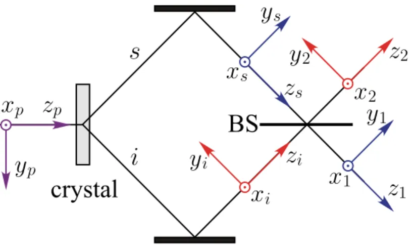
Figure 3.1: HOM interferometer. SPDC-created photons are reflected through paths s and

i onto a beam splitter (BS). The coordinate systems xt, yt, zt (t = s, i) are transmitted or reflected into coordinate systems xj, yj, zj (j= 1,2). xp, yp, zp is the coordinate system of the pump field.

3.2

Multimode Hong-Ou-Mandel interference

Consider the Hong-Ou-Mandel (HOM) interferometer shown in Fig. 3.1, in which two photons are generated by SPDC and then reflected onto opposite sides of a beam splitter. It is well known that when the paths s and i are equal, the photons can interfere. If the path length difference is greater than the coherence length of the down-converted photons, then there is no interference and the photons leave either side of the beam splitter randomly. Here we will assume that lengths of paths s and i are equal.

The two-photon detection amplitude, given by eq. (2.28), is

Ψ(r1,r2) =hvac|E(+)2 (r2)E(+)1 (r1)|ψi, (3.1)

where E(+)_l (rl) is the field operator in the paraxial approximation given by eq. (2.29) for the modelandrlis the detection position. We assume that experimental conditions are such that the two-photon state |ψi is accurately given by equation (2.24).

in input modes s and i:

a1(q, σ) =tas(qx, qy, σ) +irai(qx,−qy, σ) (3.2a) a2(q, σ) =tai(qx, qy, σ) +iras(qx,−qy, σ), (3.2b) where t and r are the transmission and reflection coefficients of the beam splitter (t2 _+r2 _{= 1). We have assumed that the beam splitter is symmetric. A field reflected}

from the beam splitter undergoes a reflection in the horizontal (y) direction, while a transmitted field does not suffer any reflection, as illustrated in Fig. 3.1. The negative sign that appears in the qy components is due to this reflection. Until now all studies of two-photon interference at a beam splitter have considered a monomode situation, in which the sign change due to this reflection does not appear.

The two-photon wave function is split into four components, according to the four possibilities of transmission and reflection of the two photons:

Ψ=Ψtr(r1,r1′) +Ψrt(r2,r′2) +Ψtt(r1,r2) +Ψrr(r1,r2), (3.3)

where tr stands for photon s transmitted and photon i reflected, etc. It is clear that only Ψtt and Ψrr are responsible for coincidence detections at D1 and D2, while Ψtr and Ψrt correspond to two photons in arm 1 and two photons in arm 2, respectively. For convenience, the four components of Ψ are written in two different coordinate systems, r₁ = (x1, y1, z1) and r2 = (x2, y2, z2), since we must work in the paraxial

approximation around two different axes z1 and z2.

3.2.1 Two-port coincidence detection

We will first focus our attention on two-port coincidence detections, which contribute to Ψ through Ψtt and Ψrr. Using (3.1), (3.2) and the field operators in the paraxial approximation (2.29), the probability amplitude to detect coincidences at output ports 1 and 2 is

Ψ(r1,r2)∝

X

s₁,s₂

s1s2

X

s_s,s_i

Cs_s,s_i

Z Z Z Z

dq₁dq₂dq_sdq_ieiq1·ρ1eiq2·ρ2eiq12z1/2k1_eiq22z2/2k2×

v(q_s+q_i)hvac_|(t2_{a1(qsx, qsy,ss)a2(qix, qiy,si)}

Using the properties of the destruction operators, the coincidence detection amplitude is

Ψ(r₁,r₂) =Ψ_tt(r₁,r₂) +Ψ_rr(r₁,r₂), (3.5)

where

Ψ_tt(r₁,r₂)∝t2 X

s₁,s₂

Cs₁,s₂s1s2

Z Z

dq1dq2eiq1·ρ1eiq2·ρ2eiq

2 1z1/2k1

eiq22z2/2k2

v(q1x+q2x, q1y+q2y) (3.6)

and

Ψ_rr(r₁,r₂)_{∝ −}r2 X

s₂,s₁

Cs₂,s₁s2s1

Z Z

dq₁dq₂eiq1·ρ1eiq2·ρ2eiq 2 1z1/2k1

eiq22z2/2k2

v(q1x+q2x,−q1y−q2y). (3.7)

Simplifying (3.6) is straightforward. Performing the change of variables

R= (Rx, Ry) =

x1+x2

2 ,

y1+y2

2

, (3.8a)

S = (Sx, Sy) = (x1−x2, y1−y2), (3.8b)

Q= (Qx, Qy) = (q1x+q2x, q1y +q2y), (3.8c)

and

P= (Px, Py) =

q1x−q2x

2 ,

q1y −q2y 2

, (3.8d)

so that dq₁dq₂ =dQdPand q_1·ρ₁+q_{2 ·}ρ₂ =Q_·R+P_·S, we have

Ψtt(r1,r2)∝t2

X

s₁,s₂

Cs₁,s₂s1s2

Z

dQv(Q)eiQ·R_eiQ2_Z 12/2K

Z

dPeiP·S_eiP2_Z

12/2K_{, (3.9)}

where Z12 is the biphoton focal distance 1 given by [77]

1 Z12 = 1 2 1 zs + 1 zi , (3.10) 1