117
APPLICATION OF THE ANALYTICAL ECT METHOD TO BCC
METALS
E Aghemenloh 1,*, S O Azi1 & S Yusuf 2 1
Department of Physics, University of Benin, Benin City, P.M.B. 1154, Edo State, Nigeria. 2
Department of Science Laboratory, Kogi State Polytechnic, Lokoja, Kogi State, Nigeria. E-mail: [email protected]
ABSTRACT
The analytical equivalent crystal theory method which is a modification of the ECT method has been used to establish a database of surface energy for the three low-index surfaces of alkali metals such as Li, Na, K, Rb, and Cs. The calculated results are in good agreement with experiment and other theoretical values. And the calculated results show that the surface energy is anisotropic. As previously predicted, the surface energy of the close-packed plane (110) is the lowest of the three low-index surfaces.
Key words: Surface energy, Analytical equivalent Crystal theory, Metals
1. INTRODUCTION
Surface energy is defined as the surface excess free energy per unit area of a particular crystal facet and is one of the basic quantities in surface physics. It determines the equilibrium shape of mezoscopic crystals, it plays an important role in faceting, roughening, and crystal growth phenomena, and may be used to estimate surface segregation in binary alloys. Most of the experimental surface energy data [1, 2] stems from surface tension measurements in the liquid phase extrapolated to zero temperature. Although these data at present form the most comprehensive experimental source of surface energies, they include uncertainties of unknown magnitude and correspond to an isotropic crystal. Hence, they do not yield information as to the surface energy of a particular surface facet. Therefore, a theoretical determination of surface energy is of vital importance.
During the last decades, there have been many calculations of the surface energy of metals either from first-principles [3-5] or by semi-empirical methods [6-8]. The latter are of course computationally highly efficient and in many cases provide a good description of the energetics of surfaces. Hence, they have been used successfully, in describing a wide range of material properties. In contrast, most first-principles methods are computationally demanding and have typically been used only for particular cases, focusing on a few elements or on a special application for a given metal surface.
The equivalent crystal theory method (ECT) since its introduction have been extensively used to describe the energetic of defects in metals [9, 10] and alloys [11, 12], and also in the study of charge transfer in metal nano-clusters [13]. More recently the ECT was extended to hcp metals to calculate surface energies [14]. However, the major constraint in the implementation of the ECT method at present is the time limiting step involved in finding the root of the equations which might be important for complex defects and large systems.
To overcome this constraint, recently Zypman and Ferrante [15] introduced an analytical algorithm to invert the ECT equations that reduces the computational speed by employing the Lambert function. This new algorithm of the ECT has successfully been applied to calculate the (100) surface energy of seven fcc metals [15], but has not been applied to bcc metals. Our aim therefore, is to extend this new ECT method to bcc metals.
The remainder of this paper is organized as follows. In section 2, we give a brief discussion of the new analytical ECT method. In section 3, we discuss the analytical ECT method of calculating the surface energies of bcc metals. The results of surface energies for 5 bcc metals are reported in section 4, along with the results obtained by other workers. Concluding remarks are giving in section 5.
2. THE ANALYTICAL ECT METHOD
In ECT the total energy of a collection of atoms in a defect is the sum of individual energy contributions U(aeq),
where aeq is called equivalent lattice parameter and U(aeq), is explicitly given by the Universal binding energy
118
from that point on the UBER. The value of aeq is obtained in terms of a0 from the inversion of the basic ECT transcendental equation. Although conceptually simple, the inversion process represents the computational time limiting step in the implementation of the algorithm.
The implementation of ECT involves a perturbation equation that determines the energy of a solid with a defect in terms of a perfect crystal of the same substance expanded or contracted from the equilibrium lattice parameter to a
new “equivalent” lattice parameter. This procedure is equivalent to finding an embedding electron density . A typical atom at a given location is embedded in a density produced by the electronic charge density of the remainder atoms in the system. The yet unknown, equivalent nearest-neighbour distance, Req satisfies
N
1R
eqpe
Req
N
2(
c
2R
eq)
pe
(1/)c2Req
(1) where N1 is the number of nearest – neighbours in the minimum energy crystal structure corresponding to that atom, N2 is the number of next-nearest neighbours, C2 is the ratio of the next-neighbour distance to the nearest-neighbour distance, and and are known material-dependent constants. In many applications of ECT to evaluate defect formation energies, on the right-hand side of Eq. (1), is written in a form similar to the left-hand side. For example, the density produced by neighbours on an atom next to a vacancy is
2 0 01 2
1 2 0
1 1
R C p
eq R
p
e
R
C
N
e
R
N
,
where
N
11
N
1
1
andN
12
N
2 because the atom in question loses one nearest-neighbour (where the vacancy is located) and no second near neighbour. In this example, the lattice is unrelaxed and consequently R0 represents the nearest neighbour distance of the perfect crystal. This shows explicitly that Req is the unknown in Eq. (1). OnceReq is obtained, ECT usess this value in the UBER function, U(aeq). The corresponding energy cost is then U(aeq)–
U(ao). In what follows, we adopt the method of Zypman and Ferrante [15].
The general problem is therefore to find the function
Req = G() (2)
Equation (1) can be cast in dimensionless form by defining eq
R
y
1 1
1 2
1
2 2
N e
y c N N e
y
p y
C p
p y
p
(3)By introducing 1 1 1 , , ,
1 21 1 2
2 N n N x
N C
p
Eq. (3) becomes
y
pe
y
1
n
21c
2py
pe
y
x
(4) The constant is about unity or larger and C2 > 1, thus > 0, which is a conservative lower bound for . By usingappropriate values from Table 1, one finds that
n
21c
2py
pe
y
0
.
25
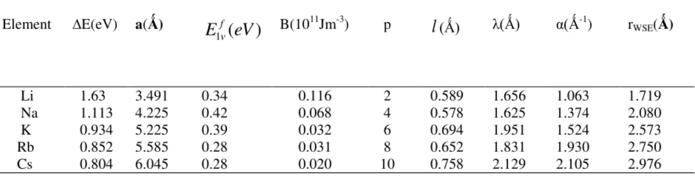
. Thus, in Eq. (4), the second term inside the parenthesis is much smaller than unity, and therefore it is dropped in many real applications. Thus, the problem reduces to finding the roots ofTable 1. Pure metal properties and the calculated ECT constants for bcc metals. Lattice constants a and cohesive
energy ∆E are from Ref. [29]; Bulk modulus B are from Refs. [16, 30] and Monovacancy formation energies f v
E
1are from Refs. [31,32].
Element ∆E(eV) a(Ǻ)
(
)
1
eV
E
fv B(1011Jm-3) pl
(Ǻ) λ(Ǻ) α(Ǻ-1) rWSE(Ǻ)Li 1.63 3.491 0.34 0.116 2 0.589 1.656 1.063 1.719
Na 1.113 4.225 0.42 0.068 4 0.578 1.625 1.374 2.080
K 0.934 5.225 0.39 0.032 6 0.694 1.951 1.524 2.573
Rb 0.852 5.585 0.28 0.031 8 0.652 1.831 1.930 2.750
119
x
e
y
p y
(5)A sketch of Eq. (5) is shown in Fig.1. In Fig.1, the root y1 corresponds to the smaller lattice parameter while the root y2 corresponds to the larger lattice parameter. Creating a vacancy effectively lowers the atom density thereby increasing y [6]. Thus the physically accepted root is y2.
Equation (5) can now be recast in the Lambert form:
p
x
e
p
y
p p y1
(6)
with the solution
(
)
1
1
p
x
pW
y
p
(7)where W-1 is the Lambert function [17,18]. The sub index “-1” labels the branches. The Lambert function has an
infinite number of complex branches with only two purely real, the branches known as “0” and “-1”.
Fig.1. Shows Eq. (5) graphically illustrating the appearance of two roots: The root �1 is to the left of the maximum that correspond to a lattice parameter smaller than
a
0,while the rooty
2 to the right corresponds to the lattice parameter larger thana
0.Define (
y
M,
x
M ) as the point corresponding to the maximum attainable density.y
M may be found by taking the maxima of Eq. (4) as
P
y
M
n
21c
2pe
yM
P
1
y
M
0
(8) Eq. (8) can be solved for as
p y p M M
M M
c
n
e
y
p
w
y
p
y
y
M
2 21 0
1
1
(9)120
1
0
2 21 0
2
Mm pPyMm Mm
c
n
e
P
y
W
y
y
p
Mm
(10)
The only non-trivial solution to Eq. (10) is for the argument of the Zero branch to be -1/e. For a complete discussion of the above equations and the conditions that lead to its derivations, the interested reader is referred to the work of Zypman and Ferrante [15], where the details can be found. According to Zypman and Ferrante, the smallest possible value of y (ymin) is given as
m in 0( 21 2 )
e c n W P y
p
(11)
Eq.(11) was used to evaluate the ymin in Table 2.
Table 2. Smallest value of y (=
y
min) and the corresponding
values for five bcc metals.
Element
y
min
(
1
1
)
c
2
1
z
n
21c
pe
yLi 1.723 0.811 0.248 Na 3.653 0.672 0.115 K 5.573 0.543 0.086 Rb 7.481 0.481 0.065 Cs 9.377 0.412 0.066
3. CALCULATION OF SURFACE ENERGY
Here, we implement the analytical algorithm of the ECT by Zypman and Ferrante. The surface energies of the three low-index planes of five bcc metals is obtained by this algorithm. However, it is emphasize that only the volume term of the ECT is retained, while neglecting the other terms. The neglect of the higher order terms of the ECT has been justified from previous studies [10, 19, 20]. In what follows we first solve Eq.(4) numerically, and then by the Lambert function as given by [15].
For the real density of the (110) plane, we notice that a typical surface atom losses 2 nearest-neighbours (out of 8 in bulk) and 2 next nearest-neighbours (out of 6 in the bulk). Then
6
R
0pexp
R
04
C
2R
0 pexp
1
C
2R
0
(12)where , and are material constants whose values depends on each metal. And C2 and R0 are given as
3
2
,
3
2
0
c
a
a
R
. Solving Eq. (12), we obtain the value of electron density Next, we solve
8
px
(13)and then
p x Log
oduct p
y
p
1
, 1
Pr (14)
Now, after obtaining the value of x from Eq. (13), we then compute the nearest neighbour distance Req from the relation
y
R
eq
(15)Once the value of y has been obtained from Eq.(14) and knowing the value of the material constant , we can then calculate the value of Req from Eq. (15). Next, we compute the lattice parameter aeq from
eq eq
c
R
121
Fortherealdensity of the (100) plane, two surfaces are involved, the surface plane (j = 1) and the first surface below the surface plane (j = 2). The equations for to be solved are:
4
R
0pexp
R
05
C
2R
0 pexp
1
C
2R
0
(17a)and
8
R
0pexp
R
05
C
2R
0 pexp
1
C
2R
0
(17b)But in the case of the (111) plane of a bcc lattice, three surfaces are involved. The surface atom losses 4 nearest – neighbours and 3 next nearest-neighbour atoms for the surface plane (j = 1). The second plane (j = 2) losses 1 nearest – neighbour atom and 3 next nearest-neighbour atoms, while the third plane (j = 3) losses only 1 nearest and next nearest-neighbour atom. Therefore, the equations to be solved are:
4
R
0pexp
R
03
C
2R
0 pexp
1
C
2R
0
(18a)
7
R
0pexp
R
03
C
2R
0 pexp
1
C
2R
0
(18b)and
7
R
0pexp
R
06
C
2R
0 pexp
1
C
2R
0
(18c) Eqs (17) and (18) are then solved for and Eqs.(13) and (14) for x and y. Thereafter, Eqs.(15) and (16) are solved for Req and aeq for each bcc metals.
Once the values of Req are known from Eq. (15), then the values of a* and F* can be calculated directly [6]. The surface energy for each of the three low-index faces is then calculated from the formulas
a
j
F
a
E
j*,
*
3
1 2 111
(19)
a
j
F
E
a
j*,
*
2
1 2110
(20)
a
j
F
E
a
E
j*,
*
1 2100
(21)The sum over j includes only one atom per atomic layer and usually only a few layer need be included for metal low index planes.
4. RESULTS AND DISCUSSION
The equivalent crystal nearest neighbour distance Req is a very vital parameter in the ECT method, since it is the parameter needed in the calculation of surface energy. Req values are also needed in the computation of aeq, the equivalent lattice parameters. These are shown in Table 3 and have been employed to calculate the values of surface energies exhibited in Table 4. Table 3 also displays the relative difference between the Lambert evaluation method (AECT) and the numerical evaluation (Newton –Raphson method) of the ECT. Table 3 provides a comparison of this present work using Lambert evaluation with a previous study [21] which used the old ECT. It can be seen from the table that there is a good agreement between the two ECT methods. Like in Table 3, the present AECT results of surface energies in Table 4 compares well with an earlier result [21].
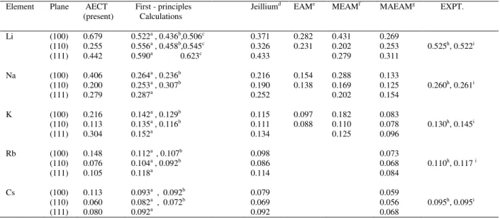
The surface energies obtained for the three low – index faces of the five bcc metals are presented in Table 5. For comparison, we also present some theoretical results and experimental derived values. These theoretical methods include, first- principles calculations in Refs.[3-5,22], the jellium model in Ref.[23] ,the embedded atom method (EAM) in Ref.[24], the modified embedded atom method (MEAM) in Ref.[25],the modified analytical embedded atom method (MAEAM) in Ref. [26], and experiment from Refs. [1,2]. The experimental values are determined from measurements of the surface tension of liquid metals extrapolated through a liquid-solid phase transition. From Table 5, it can be seen that our AECT surface energy results are uniformly larger
122
Table 3. ECT equivalent lattice parameters and the relative difference between Lambert evaluation (AECT) and numerical evaluation (ECT). J=1 layer only
Element Crystal face
(hkl) a
eq
A
a
(
)
0b eq
A
a
(
)
0)
(
0
A
a
eq
Li (100) 4.817 4.869 0.011
(110) 4.065 4.166 0.024
(111) 4.906 4.954 0.010
Na (100) 5.826 5.852 0.004
(110) 4.999 5.059 0.012
(111) 5.883 5.907 0.004
K (100) 7.080 7.103 0.003
(110) 6.174 6.231 0.009
(111) 7.136 7.158 0.003
Rb (100) 7.169 7.182 0.002
(110) 6.381 6.413 0.005
(111) 7.199 7.212 0.002
Cs (100) 7.778 7.794 0.002
(110) 6.959 7.001 0.006
(111) 7.818 7.833 0.002
aNew ECT method, using analytical Lambert evaluation [15 ] bOld ECT method, using numerical evaluation [21]
where
b
eq a eq b eq eq
a
a
a
A
a
(
)
(
)
0
and closer to experiment and first-principles calculations. It must be pointed out that experimental
Table 4. Rigid Surface energies for low-index bcc metals.
Element Crystal face (hkl)
AECT eV/atom Jm-2
ECTa eV/atom Jm-2
Li (100) 0.366 0.679 0.369 0.685 (110) 0.137 0.255 0.180 0.334 (111) 0.238 0.442 0.276 0.512
Na (100) 0.321 0.406 0.318 0.403 (110) 0.158 0.200 0.177 0.225 (111) 0.220 0.279 0.241 0.305
K (100) 0.261 0.216 0.254 0.211 (110) 0.137 0.113 0.150 0.124 (111) 0.367 0.304 0.197 0.164
Rb (100) 0.204 0.148 0.205 0.149 (110) 0.104 0.076 0.111 0.081 (111) 0.145 0.105 0.152 0.111
Cs (100) 0.182 0.113 0.179 0.111 (110) 0.097 0.060 0.104 0.064 (111) 0.129 0.080 0.138 0.086
123
measurements of the surface energy are more commonly found for polycrystalline materials. In the present calculation, the relaxation and reconstruction of the atomic positions are neglected, which may lead to errors of up to a few percent.
Table 5. Experimental and theoretical surface energies ( in Jm-2) for bcc metals.
Element Plane
AECT (present)
First - principles Calculations
Jeilliumd EAMe MEAMf MAEAMg EXPT.
Li (100) 0.679 0.522a , 0.436b,0.506c 0.371 0.282 0.431 0.269
(110) 0.255 0.556a , 0.458b,0.545c 0.326 0.231 0.202 0.253 0.525h, 0.522i
(111) 0.442 0.590a 0.623c 0.433 0.279 0.311
Na (100) 0.406 0.264a , 0.236b 0.216 0.154 0.288 0.133
(110) 0.200 0.253a , 0.307b 0.190 0.138 0.169 0.125 0.260h, 0.261i
(111) 0.279 0.287a 0.252 0.202 0.154
K (100) 0.216 0.142a , 0.129b 0.115 0.097 0.182 0.083
(110) 0.113 0.135a , 0.116b 0.111 0.088 0.110 0.078 0.130h, 0.145i
(111) 0.304 0.152a 0.134 0.125 0.096
Rb (100) 0.148 0.112a , 0.107b 0.098 0.073
(110) 0.076 0.104a , 0.092b 0.086 0.068 0.110h, 0.117 i
(111) 0.105 0.118a 0.114 0.084
Cs (100) 0.113 0.093a , 0.092b 0.079 0.059
(110) 0.060 0.082a , 0.072b 0.069 0.056 0.095h, 0.095i
(111) 0.080 0.092a 0.092 0.068
a
FCD calculations, Ref.[5] b
LMTO-ASA calculations, Ref. [3] c
Pseudopotential calculations, Ref. [22] d
Jellium calculations, Ref. [23] e
Embedded atom method calculations, Ref. [24] f
modified embedded atom method calculations, Ref. [25] g
Modified analytical embedded atom method calculations, Ref. [26] h
Experiment, Ref. [2]; i Experiment, Ref. [1]
For all the theoretical models whose results are presented in table 5, the high density (110) surface has the lowest energy in all cases, except Na and Li where Refs. [3, 5] predicts that
100
110 .So from surface energy minimization, the (110) texture should be favourable in the bcc film. This is consistent with experimental results [27, 28]. From Table 5, it is clearly seen that the calculated surface energy shows a strong anisotropy, the surface energy values of (100), (110) and (111) surface are different. Particularly puzzling is the fact that while the first-principles calculations[3, 5] results for Na [5], K, Rb, Cs, conform to the expected order of
110
100 for the bcc metals, their results for Li, Na [3], is the reverse. It is important to note that all of the AECT surface energy results from this study consistently support the trend 110 < 111 < 100 for bcc metals. This is also the trend obtained by MEAM [25]. However, the results of the other theoretical model in Table 5 do not always support this trend. In fact, the jellium model [23] and MAEAM model [26] has
111
100. We are unable to attribute the reason for these differences to the relaxation effects which were ignored in this study, since contributions from relaxation effects are usually small [10, 6, 19]. The absence of a common trend in the ordering of the (100), (110) and (111) surface energies amongst the various theoretical models is a problem yet to be satisfactorily discussed.5. CONCLUSIONS
We have in this study employed the new analytical equivalent crystal theory method to provide a set of surface energy for bcc metals. In this work three surfaces were considered for the five bcc metals. These are the (100), (110) and the (111) surfaces. We have successfully extended the surface energy results of the AECT method first proposed by Zypman and Ferrante [15] for fcc only to bcc metals.
124
packed bcc (110) surface posses the lowest energy. Our surface energy results do not include relaxation effects but this is currently being studied and whatever findings we obtain will be reported.
6. ACKNOWLEDGEMENTS
The authors would like to acknowledge fruitful discussion with Dr. E. O. Aiyohuyin.
7. REFERENCES
[1]. W.R. Tyson, W.A. Miller, Surf. Sci. 62 (1977) 267.
[2]. F.R. deBoer, R. Boom, W.C. M. Mattens, A. R. Miedema, A. K. Niessen, Cohesion in Metals North-Holland, Amsterdam, 1988.
[3]. H.L.Skriver, N.M. Rosengaard, Phys. Rev. B46 (1992) 7157.
[4]. M. Methfessel, D. Henning, M. Scheffler, Phys. Rev. B46 (1992) 4816. [5]. L.Vitos, A.V. Ruban, H.L. Skriver, J. Kollar, Surf. Sci. 411 (1998) 186.
[6]. J.R.Smith, T. Perry, A. Banerjea, J. Ferrante, G. Bozzolo, Phys. Rev. B 44 (1991) 6444. [7]. S.M. Foiles, M.I. Baskes, M.S. Daws, Phys. Rev. B 33 (1986) 7893.
[8]. M.W. Finnis, J. E. Sinclair, Philos. Mag. A 50 (1984) 45 . [9]. S.V. Khare, T.L. Einstein, Surf. Sci. 314 (1994) 857.
[10]. A.M. Rodriguez, G. Bozzolo, J. Ferrante, Surf. Sci. 289 (1993)100. [11]. G. Bozzolo, J. Ferrante, J.R. Smith, Phys. Rev. B 45 (1992) 493.
[12]. G. Bozzolo, J.E. Garces, R.D. Noebe, D, Farias Nanotechnology 14 (2003) 939.
[13]. A.I. Frenkel, L.D. Menard, P. Northrup, J.A. Rodriguez, F. Zypman, D. Glasner, S –P. Gao, H. Xu, J.C. Yang, R.G. Nuzzo in: B. Hedman, P.Pianetta (Eds), X-ray Absorption Fine Structure-XAFS13, Vol.882, American Institute of Physics 2007 749.
[14]. E. Aghemenloh, J.O.A. Idiodi, S.A. Azi, Comput. Mater. Sci. 46 (2009) 524. [15]. F.R. Zypman, J. Ferrante, Comput. Mater. Sci. 42 (2008) 659.
[16]. J.H. Rose, J.R. Smith, J. Ferrante, Phys. Rev. B28 (1983)1835; J.H. Rose, J.R. Smith, J. Ferrante, Phys. Rev. B29 (1984) 2963.
[17]. F. Chapeau-Blondeau, IEEE Trans. Signal Proc. 50 (2002) 2160. [18]. B. Hayes, American Scientist 93 (2005)104.
[19]. P.J. Feibelman, Phys. Rev. B 46 (1992) 2532.
[20]. M. Mansfield, R.J. Needs, Phys. Rev. B 43 (1991) 8829.
[21]. E. Aghemenloh, J.O.A. Idiodi, J. Nig. Ass. Math. Phys. 5 (2001) 101. [22]. K. Kokko, P.T. Salo, R. Laihia, K. Mansikka, Surf. Sci. 348 (1996) 168. [23]. J.P. Perdew, H.Q.Trans, E.D. Smith, Phys. Rev. B 42 (1990) 11627. [24]. A.M. Guellil, J.B. Adams, J. Mater. Res. 7 (1992) 639.
[25]. M.I. Baskes, Phys. Rev. B 46 (1992) 2727.
[26]. Y.N. Wen, J. M. Zhang, J. Comput. Mater. Sci. 42 (2008) 281. [27]. B.E. Sundquist, Acta Metall. 12 (1964) 670.
[28]. H.E. Grenga, R. Kumar, Surf. Sci. 61 (1976) 283. [29]. G. Bozzolo, J. Ferrante, Phys. Rev. B 46 (1992) 8600.
[30]. C. Kittel, Introduction to Solid State Physics, 5th ed. (Wiley, New York, 1976) p.85. [31]. T. Korhonen, M.J. Puska, R.M. Mieminen, Phys. Rev. B 51 (1995) 9526.