Abstract—In this paper, a novel learning framework for Single hidden Layer Feed forward Neural network (SLFN) called Optimized Extreme Learning Machine (OELM) is proposed for the classification of EEG signals with the emphasis on epileptic seizure detection. OELM is an effective learning algorithm of single-hidden layer feed-forward neural networks. It requires setting the number of hidden neurons and the activation function. Adjustment in the input weights and hidden layer’s biases are not needed during the implementation of the algorithm, and only one optimal solution is produced. This makes the OELM a valuable tool for the applications that need small response time and provide a good accuracy. The features such as energy, entropy, maximum value, minimum value, mean value and standard deviation of wavelet coefficients are used to represent the time frequency distribution of the EEG signals in each sub-band of the Wavelet Transformation. We have compared the proposed classifier with other traditional classifiers by evaluating it with the benchmark EEG dataset. It is found that the performance of the proposed OELM with Wavelet based statistical features is better in terms of training time and classification accuracy. An accuracy of 94% for classifying the epileptic EEG signals is achieved and needs less training time compared with SVM.
Index Terms—EEG Signal Classification, Epileptic Seizure Detection, Optimized Extreme Learning Machine, Wavelet Transformation
I. INTRODUCTION
HE human brain is obviously a complex system, and exhibits rich spatiotemporal dynamics. Epilepsy is one of the most prevalent neurological disorders in human beings. It is characterized by recurring seizures in which abnormal electrical activity in the brain causes the loss of consciousness or a whole body convulsion. Patients are often unaware of seizure, because it is unpredictable and it may result in severe physical injury. Studies show that 4-5% of the total world population has been suffering from epilepsy [1].
Electroencephalogram is one of the important tools for diagnosis and analysis of epilepsy. Electroencephalogram is a recorded representation of electrical activity produced by firing of neuron within the brain along the scalp. For recording EEG, electrodes will be pasted at some key points on the patient’s head. Electrodes pick up the signals and will be recorded in a device through wires that are connected to
Manuscript received February 27, 2014; revised September 17, 2014. A.S. Muthanantha Murugavel is Assistant Professor (SG) with Department of Information Technology, Dr.Mahalingam College of Engineering and Technology, Pollachi-642003, Tamilnadu, India, (phone: 91-9894839142; fax: 91-236070; e-mail: [email protected]).
S. Ramakrishnan is Professor & Head with Department of Information Technology, Dr.Mahalingam College of Engineering and Technology, Pollachi-642003, Tamilnadu, India (e-mail: [email protected]).
electrodes. The “10-20” system is the internationally recognized method to apply the location of electrodes in EEG recording. The“10-20” refers to the fact that actual distances between electrodes are either 10% or 20% of front-back or right-left distance of the skull [2–4].
As complete visual analysis of EEG signal is very difficult, automatic detection is preferred. Fourier transform has been most commonly used in early days for processing EEG signals. However as EEG signal is a non-stationary signal, Fourier analysis does not give accurate results [5–7]. The most effective time-frequency analysis tool for analysis of transient signal is wavelet transform [8–10].
The automated diagnosis of epilepsy can be subdivided into preprocessing, feature extraction, and classification. Seizure detection can be classified as either seizure onset detection or seizure event detection. In seizure onset detection the purpose is to recognize the starting of seizure with the shortest possible delay. The purpose of seizure event detection is to identify seizures with the highest possible accuracy [11–16].
For treatment of epilepsy, patients take antiepileptic drugs on daily basis. But about 25% of them again experience frequent seizures. For these patients, surgery is the most important and generally adopted treatment method. Surgery can be done only if epileptogenic focus is identified accurately. For this purpose different types of tracers are used as soon as seizure onset is detected. Hence the seizure onset detection is very important [1].
Seizure detection from EEG signal was started since 1980s. In 1982 Gotman proposed a remarkable work on seizure detection [5]. Khan and Gotman proposed a wavelet based method for classification of epileptic and non-epileptic data [17]. In 2005 wavelet transform method and short time Fourier transform method were compared to find out their accuracy in determining the epileptic seizures. They found that wavelet transform method gives better performance [18]. Ubeyli suggested the combined neural network model for the classification using wavelet based features [12]. Their method gave good accuracy in Bonn University data. In 2011, Gandhi et al. made a comparative study of wavelet families for EEG signal classification [11]. Important features such as energy, entropy, and standard deviation at different subbands were computed using wavelet decomposition. Feature vector was used to model and train the probabilistic neural network and classification accuracies were evaluated for each of the wavelet families. The result obtained was compared with support vector machine classifier.
An onset detection system was designed by Gotman and Saab in 2004. They achieved a median detection delay of 9.8 sec and sensitivity of 77.9% using scalp EEG. Shoeb and
An Optimized Extreme Learning Machine for
Epileptic Seizure Detection
A. S. Muthanantha Murugavel, Member, IAENG, and S. Ramakrishnan, Member, IAENG
Guttag achieved 96% sensitivity and small detection delays [6]. Sorensen et al. achieved 78–100% sensitivity when using a matching pursuit algorithm and with 5–18 seconds delay in seizure onset detection [19].
Neural networks and statistical pattern recognition methods have been applied to EEG analysis. Over the past two decades, single hidden layer feed-forward neural networks (SLFNs) have been used for classification. Classification is the basis of cognition. Of all the algorithms, neural networks, which simulate the function of neurons simply, have been proved to be a general and effective method [20]. The learning speed of feed-forward neural networks is in general far slower than required and it has been a major bottleneck in their applications during past decades. Recently, an effective training algorithm for SLFNs called Hybrid Online Sequential Extreme Learning Machine (HOS-ELM) is proposed in [21]. In contrast to the standard ELM, which involves a trial-and error process to identify a suitable architecture of the network, Optimized Extreme learning machine (OELM) searches for a suitable network architecture, i.e., identifying an appropriate number of hidden nodes for the data set in hand, based on statistical information, hence there is significant saving in training time. For further improving its search performance, a cooperative PSO method called multiple particle swarm optimizers with inertia weight (MPSOIW) is proposed in [22]. Furthermore, OELMs produce significantly more compact networks, compared with the standard ELM, through the removal of irrelevant hidden nodes. In comparison to the standard ELM, OELMs is also not affected by the functional form of the hidden node used. Hence OELMs demonstrate excellent robustness in the generalization ability of the final network. However it is also found that OELM requires more hidden neurons than conventional tuning-based algorithms in many cases. This algorithm can obtain good performance with high learning speed in many applications. Using statistical methods to measure the relevance of each hidden node in contributing to the prediction accuracy of the classifier, the appropriate architecture of the classifier network is then defined. A pruned-ELM (P-ELM) algorithm [23] is a systematic and automated approach for designing ELM classifier network. P-ELM uses statistical methods to measure the relevance of hidden nodes. Initially large number of hidden nodes, irrelevant nodes, is then pruned by considering their relevance to the class labels. As a result, the architectural design of ELM network classifier can be automated. Gaurang Panchal et al., [24] put forth a behavior analysis of multilayer perceptrons with multiple hidden neurons and hidden layers. The problem with the model selection is considerably important for acquiring higher levels of generalization capability in supervised learning. A computer-aided classification system has been developed for cyst and tumor lesions in dental panoramic images [25]. This paper is intended to compare the performance of four different types of fuzzy aggregation methods in classification of epilepsy risk levels from EEG Signal parameters [26].
In this paper, a novel learning framework for SLFNs called optimized extreme learning machine (OELM) is proposed. This frame work uses the same concept of the
ELM where the output weights are obtained using least squares, however, with the difference that Tikhonov's regularization is used in order to obtain a robust least square solution. The problem of reduction in the ELM performance in the presence of irrelevant variables is well known, as well as its propensity for requiring more hidden nodes than conventional tuning-based learning algorithms. To solve these problems, the proposed framework uses an optimization method to select the set of input variables and the configuration of the hidden-layer. Furthermore, in order to optimize the fitting performance, the optimization method also selects the weights of connections between the input layer and the hidden-layer, the bias of neurons of the hidden-layer, and the regularization factor. Using this framework, no trial-and-error experiments are needed to search for the best SLFN structure. Selection of the optimal number of neurons in this layer and the activation function of each neuron, try to overcome the propensity of ELM in necessitating more hidden nodes than conventional tuning-based learning algorithms.
The paper is organized as follows. The overall system is explained in Section 2. Section 3 presents the proposed methodologies such as Wavelet Transform based feature extraction and Optimized Extreme Learning Machine based Classification of EEG signals with the emphasis on epileptic seizure detection. Section 5 discusses the experimental results and findings. Finally section 6 concludes the paper.
II. MATERIALS AND METHODS
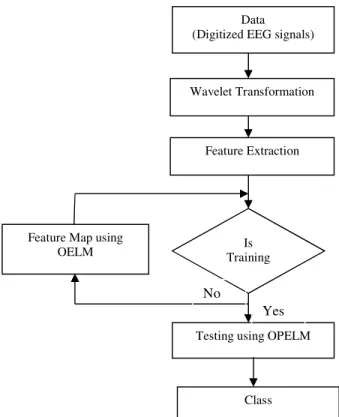
As in traditional pattern recognition systems, the epileptic seizure detection consists of main modules such as a feature extractor that generates a Wavelet based statistical features from the EEG signals and a feature classifier (OELM) that outputs the class. The block diagram of the proposed approach is illustrated in Fig. 1.
Fig. 1. Block diagram of the proposed EEG classification system.
Data (Digitized EEG signals)
Wavelet Transformation
Feature Extraction
Is Training
Testing using OPELM Feature Map using
OELM
Class
TABLEI
DESCRIPTION SUMMARY OF EEG DATA SET OBTAINED FROM UNIVERSITY OF BONN GERMANY
Subject
SET A SET B SET C SET D SET E
Five healthy subject Five epileptic patients
Patient state Awake and eyes open (normal)
Awake and eyes
closed (normal)
Seizure free
(interictal)
Seizure free
(interictal)
Seizure
activity(ictal)
Electrode types Surface Surface Intracranial Intracranial Intracranial
Electrode
placement International 10–20 International 10–20
Within epileptogenic
zone
Opposite to
epileptogenic zone
Within epileptogenic
zone
No. of epochs 100 100 100 100 100
Epoch duration (s) 23.6 23.6 23.6 23.6 23.6
A. Dataset Description
The EEG data [27] used in this work is obtained from University of Bonn, Germany. The data is available in public domain that consists of five different sets. Each data set consists of 100 single-channel EEG epochs of 23.6 s duration. The data were recorded with 128-channel amplifier system and digitized at 173.61 Hz sampling rate and 12-bit A/D resolution. The description of the data set is summarized in Table I.
B. Wavelet Transformation
Wavelet transform is the representation of a time function in terms of simple, fixed building blocks termed as wavelets. These building blocks are a family of functions which are derived from a single generating function called mother wavelets using translation and dilation operations. The main advantage of wavelet transform is that it has varying window size, being broad at low frequency and narrow at high frequency. It leads to an optimal time-frequency resolution in all frequency ranges. By performing spectral analysis using wavelet transform, EEG signals consisting of many data points can be compressed into a few features [28].
The key feature of wavelets is the time-frequency localization. It means that most of the energy of the wavelet is restricted to a finite time interval. A newer alternative to the wavelet transform is the Wavelet transform. Wavelets are very similar to wavelets but have some important differences. In particular, whereas wavelets have an associated scaling function φ (t) and wavelet function ψ (t), Wavelets have two or more scaling and wavelet functions. For notational convenience, the set of scaling functions can be written using the following vector notation.
φ(t) ≡ [φ1(t)φ2(t)⋯φr(t)]T (1) where is called the multi scaling function. Likewise, the Wavelet function is defined from the set of wavelet functions as
ψ(t) ≡ [ψ1(t)ψ2(t)⋯ψ r(t)]T (2) when r=1. ψ (t), is called a scalar wavelet, or simply wavelet. While in principle it can be arbitrarily large, the Wavelets studied to date are primarily for r=2. Wavelet transformation employs two sets of functions called scaling functions and wavelet functions, which are related to low-pass and high-low-pass filters respectively. The decomposition
of the signal into the different frequency bands is merely obtained by consecutive high-pass and low-pass filtering of the time domain signal. The procedure of multi resolution decomposition of a signal s[n] is schematically shown in Fig. 2. Each stage of this scheme consists of two digital filters and two down-samplers by 2. The first filter, h[n] is the discrete mother wavelet, high pass in nature, and the second, g[n] is its mirror version, low-pass in nature. The down-sampled outputs of first high-pass and low-pass filters provide the detail, D1 and the approximation, A1, respectively. Table II summarizes various wavelet decomposed signal sub-bands and its frequency ranges. Wavelet transformation have advantages over traditional Fourier transforms for representing functions that have discontinuities and sharp peaks, and for accurately deconstructing and reconstructing finite, non-periodic and/or non-stationary signals.
Fig. 2. Four Level Wavelet Decomposition.
TABLEII
WAVELET DECOMPOSED SIGNAL SUB-BANDS AND ITS FREQUENCY RANGES
Decomposed signal Frequency Range (Hz)
D1 43.4-86.8
D2 21.7-43.4
D3 10.8-21.7
D4 5.4-10.8
A4 0-5.4
Wavelets have several advantages in comparison to scalar wavelet, which can possess compact support, orthogonality, symmetry and high order approximation, which is not possible with scalar wavelet. We experimentally found that Wavelet provides superior performance over scalar wavelet for classification of EEG signals
C. Parameters for Feature Extraction
based features and some statistical features without wavelet decomposition.
Wavelet Based Features such as Energy, Entropy, Standard Deviation, Mean, Maximum, and Minimum were used as parameters after wavelet decomposition.
The energy at each decomposition level was calculated as = ∑ , = 1,2, ⋯ , , (3)
= ∑ . (4)
The entropy at each decomposition level was calculated as = ∑ log , = 1,2, ⋯ , , (5)
where = 1, 2, . . . , is wavelet decomposition level from 1 to and is the number of coefficients of detail or approximation at each decomposition level.
The standard deviation at each decomposition level was calculated using the following equation:
= ∑ − ! / , (6)
where is the mean and is given by
= ∑ , = 1,2, ⋯ , , (7)
D. Feature Classification
Feed forward neural networks have been extensively used in many fields because of their ability: To approximate complex nonlinear mappings directly from the input samples; To provide models for a large class of natural and artificial phenomena that are difficult to handle using classical parametric techniques. On the other hand, neural networks lack faster learning algorithms. The traditional learning algorithms are usually far slower than required. It may take several hours, several days, and even more time to train neural networks by using traditional methods. From mathematical point of view, research on the approximation capabilities of feed forward neural networks has focused on two aspects: universal approximation on compact input sets and approximation in a finite set of training samples. Two main architectures exist for Single Layer Feed forward Neural network (SLFN), namely: 1) those with additive hidden nodes, and 2) those with Radial Basis Function (RBF) hidden nodes. For many of the applications using SLFNs, training methods are usually of batch-learning type. The SLFNs can approximate any function with arbitrarily small error and form boundaries with arbitrary shapes if the activation function is chosen properly. Hence, in applications of function approximation and classification, the SLFN is one of powerful tools which can be used. Different from the tenet in neural networks, all the hidden nodes in SLFNs need to be tuned.
E. Extreme Learning Machine (ELM)
An effective training algorithm for SLFNs called Extreme Learning Machine (ELM) shows that the hidden
nodes of generalized feed forward networks needn’t be tuned and these hidden nodes can randomly be generated. The Fig. 3 illustrates the general architecture of ELM. Unlike gradient-descent based algorithms, the network parameters in ELM are determined in single steps. The input weights and hidden layer biases are chosen randomly, and then the output weights are calculated by Moore–Penrose (MP) generalized inverse. This algorithm can obtain good performance with high learning speed in many applications.
For nearly all problems, one hidden layer is sufficient. Two hidden layers are required for modeling data with discontinuities such as a saw tooth wave pattern. Using two hidden layers rarely improves the model, and it may introduce a greater risk of converging to a local minima. There is no theoretical reason for using more than two hidden layers. One of the most important characteristics of a perceptron network is the number of neurons in the hidden layer. Using too many neurons in the hidden layers can result in several problems. First, too many neurons in the hidden layers may result in over fitting. Over fitting occurs when the neural network has so much information processing capacity that the limited amount of information contained in the training set is not enough to train all of the neurons in the hidden layers. A second problem can occur even when the training data is sufficient. An inordinately large number of neurons in the hidden layers can increase the time they take to train the network. The amount of training time can increase to a point that it is impossible to adequately train the neural network [15]. Obviously, some compromise must be reached between too many and too few neurons in the hidden layers. There are many rule-of-thumb methods for determining the correct number of neurons to use in the hidden layers, such as the following:
• The number of hidden neurons should be between the size of the input layer and the size of the output layer. • The number of hidden neurons should be 2/3 the size of
the input layer, plus the size of the output layer. • The number of hidden neurons should be less than
twice the size of the input layer.
III. PROPOSED METHODOLOGY
A. Adjustable Single hidden Layer Feed forward Neural network (A-SLFN) architecture
The neural network considered in this paper is a SLFN with adjustable architecture as shown in Fig. 3, which can be mathematically represented by
of the hidden layer and the activation function of the output neuron, respectively. si is a binary variable used in the selection of the input variables during the design of the SLFN.
Using the binary variable si, i=1,…,n, each input variable may be considered. However, the use of variables si is not the single tool to optimize the structure of the SLFN. The configuration of the hidden layer can be adjusted in order to minimize the output error of the model. The activation function fj(
.
), j=1,…,h, of each hidden node can be either zero, if this neuron is unnecessary, or any (predefined) activation function.
A SLFN with randomly chosen weights between the input layer and the hidden layer and adequately chosen output weights are universal approximators with any bounded non-linear piecewise continuous functions.
Fig. 3. Single hidden layer feed forward neural network with adjustable architecture.
Considering that N samples are available, the output bias is zero, and the output neuron has a linear activation function, (3) and (4) can be rewritten as
# = /(01231, (10) where # = 4#/13, ⋯ , #/ 351 is the vector of outputs of the SLFN, (&= 4(&, ⋯ , ()& 51 is the vector of output weights, and v is the matrix of the outputs of the hidden neurons (3) given by
2 = 6* /13 * /23 ⋯ * / 3⋮ ⋮ ⋱ ⋮
* /13 * /23 ⋯ * / 39, (11) with si=1, i=1,…,n. Considering that the input weights and bias matrix W,
: = ;
% % ⋯ %) ( ( ⋯ ()
⋮ ⋮ ⋱ ⋮ (, (, ⋯ (,)
<, (12)
is randomly assigned, the output weights vector wO is estimated as
(= = 2& >#?, (13) where V† is the Moore–Penrose generalized inverse of the
hidden- layer output matrix V, and
#?= 4#?/13, ⋯ , #?/ 351 is the desired output. Considering that 2 ∈ ℜ B, with N≥h and rank (v)=h, the Moore– Penrose generalized inverse of V can be given by
2>= /2123 21. (14) the estimation of wO can be obtained by the following least-squares solution:
(= = /2& 123 21#?. (15) In Optimized ELM, the weights of the output connections are obtained using the same ELM methodology, however, with a change. The objective of the least squares method is to obtain the best output weights by solving the following problem:
C D/‖# − #?‖ 3, (16) where ǁ . ǁ2 is the Euclidean norm. The minimum-norm solution to this problem and the use of least squares can be considered as a two-stage minimization problem involving the determination of the solutions, and the solution with minimum norm among solutions obtained in the previous stage. The use of Tikhonov's regularization allows the transformation of this two-stage problem into a single-stage minimization problem defined by
C D/‖# − #?‖ + F‖:&‖ 3, (17) where α>0 is a regularization parameter.
(= = /2& 1 2 + FG3 21 #?, (18) where I is the hxh identity matrix. Furthermore, using Tikhonov's regularization, the robustness of the least squares solution against noise is improved. As previously mentioned, the ELM requires more hidden nodes than conventional tuning-based algorithms. Furthermore, the presence of irrelevant variables in the training dataset causes a decrease in the performance. To overcome these problems, in OELM the determination of the set of input variables, the number and activation function of the neurons in the hidden layer, the connection weights between the inputs and the neurons of the hidden layer, the bias of the hidden layer neurons, and the regularization parameter α is made using an optimization methodology. The optimization of the SLFN consists in minimizing the following evaluation function: H = IJKL/#, #?3, (19) where IJKL/#, #?3 = M ∑ 4#/N3 − #O ?/N35
overlap with the training dataset. In the optimization process, it is considered that the individual / state will be constituted by
PO= 4( , ⋯ , (,) , % , ⋯ , %) , - , ⋯ , -) , -Q , ⋯ , -)Q, F51; (20) N = 1, ⋯ , C, where -Q∈ S0,1,2U, V = 1, ⋯ , ℎ, an integer variable that defines the activation function fj of each neuron j of the hidden-layer as follows:
+ /*3 = X Y
Z0 + -Q= 0, / [\]^/ _33 + -Q= 1, * + -Q= 2,
(21)
The use of parameters -Q makes it possible that the adjustment of the number of neurons (if -Q= 0 the neuron is not considered), and the activation function of each neuron (sigmoid or linear function) take place. In this work only these two types of activation function have been used; however, any type of activation function can be considered. This optimization problem is a problem where the decision variables area is a combination of real, integer, and binary variables. The decision variables are mapped into real variables within the interval [0,1] and before computing the evaluation function for each individual, all variables need to be converted into their true value. If the true value of the l-th variable (l=1,2,⋯,v) of individual k is real, it is given by `Oa= `bJcd− `bJ , POa+ `J ,, (22)
Where `bJ , and `bJcd represent the true variable bounds (`bJ ,≤ `Oa≤ `bJcd). If it is a integer value,
`Oa= rounddown `bJcd− `bJ ,+ 1 POa! + `J ,, (23)
where rounddown(.) is a function that rounds to the greatest integer that is lower than or equal to its argument. If the true value is binary, it is given by
`Oa= round POa , (24)
where round(.) is a function that rounds to the nearest integer. The variables si, i=1,…,n, are binary variables and thus are converted using (18). The variables -Q, j=1,…,h, are integer variables and thus are converted using (17), considering that the lower and upper bounds are 0 and 2, respectively. The input weights wij and bias bj are converted using (16), considering that the lower and upper bounds are -1 and 1, respectively. Finally, the regularization parameter is also converted using (16), considering that the lower and upper bounds are 0 and100, respectively.
B. Learning model
Given a training set N={(Xi,ti)|XiєR n
, ti єR m
,i=1,..,N}, hidden node output function G(a,b,x) and the number of hidden nodes L,
• Assign randomly hidden node parameters(a i,bi),i=1,..,L • Calculate the hidden layer output matrix H
• Calculate the output weight β: β=H†T where H†is the Moore-Penrose generalized inverse of hidden layer output matrix H
TABLEIII
COMPARISON OF VARIOUS PARAMETERS FOR ELM,MLP,SVM ON TESTING SAMPLES
ELM MLP SVM
Training time(s) 2.22 1026.12 3436.62
Training error (RMSE) 0.26 0.28 0.29
Testing time(s) 0.04 0.12 0.32
Testing error (RMSE) 0.41 0.45 0.47
The number of hidden neurons /the number
of support vectors
370 620 1120
C. Comparison of ELM with BP, MLP, SVM
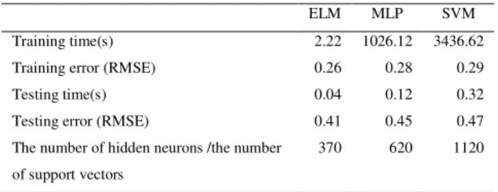
We have compared ELM with BP, MLP and SVM by evaluating with benchmark EEG dataset. Table III compares various parameters for the classifiers such as ELM, MLP and SVM on testing samples and the features of ELM have been listed below.
• ELM needs much less training time compared to popular BP and SVM
• The prediction accuracy of ELM is usually slightly better than BP.
• Compared with BP, ELM can be implemented easily since there is no parameter to be tuned except an insensitive parameter L.
• ELM needs more hidden nodes than BP but much less nodes than SVM which implies that ELM and BP have much shorter response time to unknown data than SVM From Table 2 we can see that, ELM with much lesser number of hidden neurons has a similar learning performance with SVM (ELM uses 370 hidden neurons, MLP uses 620 hidden neurons and SVM produces 1120 support vectors), the training error difference of ELM and SVM algorithms is about 0.028 and difference of ELM and MLP is about 0.0127; the testing error only has about 0.0011 and 0.0323 difference.
D. Problem of ELM with irrelevant variables
ELM models tend to have problems when irrelevant or correlated variables are present in the training data set. For this reason, it is proposed in the OELM methodology, to perform a pruning of the irrelevant variables, via pruning of the related neurons of the SLFN built by the ELM.
E. Optimized Extreme Learning Machine
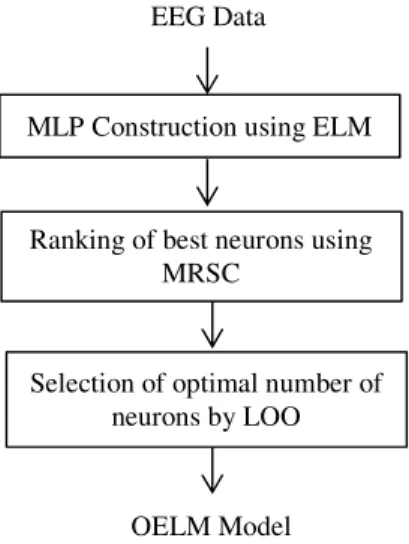
Fig. 4. The steps of OELM algorithm.
It starts with a large network and then eliminates the hidden nodes that have low relevance to the class labels. OELM mainly focuses on pattern classification applications. OELM is applicable for both regression and classification applications. Optimized-ELM algorithm is a systematic and automated approach for designing ELM classifier network. It is a very good compromise between the speed of the ELM and the accuracy and robustness of much slower and complicated methods. Fig. 4 illustrates the steps of OELM algorithm. OELM provides a systematic approach for designing the network architecture of the ELM classifier. Using statistical methods to measure the relevance of each hidden node in contributing to the prediction accuracy of the classifier, the appropriate architecture of the classifier network is then defined. The OELM methodology can also handle multiple-output—multiple- class problems in both regression and classification using multiple inputs. The accuracy of the ELM can be problematic in many cases, while the OELM remains robust to all tested data sets. The main goal in this brief was not to show that the OELM is the best either in terms of MSE or the computational time. The main goal is to prove that it is a very good compromise between the speed of the ELM and the accuracy and robustness of much slower and complicated methods.
F. OELM Algorithm
The OELM methodology has the following steps: • Build the SLFN using the original ELM algorithm • Rank the hidden nodes by applying multi-response
sparse classification algorithm
• Select the hidden nodes through Leave-One-Out (LOO) validation.
G. Multilayer perceptrons (MLPs) construction using ELM
The very first step of the OELM methodology is the actual construction of the SLFN using the original ELM algorithm with a lot of neurons (Christian et al. 2010). Multilayer perceptrons (MLPs) are feed forward neural networks trained with the standard back propagation algorithm. They are supervised networks so they require a desired response to be trained. They learn how to transform input data into a desired response, so they are widely used
for pattern classification. Their main advantages are that they are easy to use, and that they can approximate any input/output map. The main novelty introduced by the ELM is in the determination of the kernels, initialized randomly. While the original ELM used only Sigmoid kernels, Gaussian, Sigmoid and Linear are proposed in OELM. The linear kernels included in the network helps when the problem is linear or nearly linear. The Gaussian kernels have their centers taken randomly from the data points, similarly the widths randomly drawn between percentile 20% and percentile 80% of the distance distribution of the input space. From a practical point of view, it is advised to set the number of neurons clearly above the number of the variables in the dataset, since the next step aims at pruning the useless neurons from the hidden layer. Output weights b can be computed from hidden layer output matrix H: the columns hi of H are computed by hi= Ker(xi
T
), where Ker stands for either linear, sigmoid or Gaussian activation functions (including multiplication by first layer weights). Finally, the output weights b are computed by b = H†y, where H† stands for the Moore-Penrose inverse and y = (y1,
. . . , yM) T
is the output.
H. Multi-response Sparse Classification (MRSC)
It is used for the removal of the useless neurons of the hidden layer. MRSC is mainly an extension of the least angle regression algorithm (Efron et al., 2004) and hence, it is actually a variable ranking technique, rather than a selection one. An important detail shared by the MRSC and the LARS is that the ranking obtained is exact, if the problem is linear. In fact, this is the case with the OELM, since the neural network built in the previous step is linear between the hidden layer and the output. Therefore, the MRSR provides an exact ranking of the neurons for our problem. Because of the exact ranking provided by the MRSR, it is used to rank the kernels of the model. MRSR algorithm enables to obtain a ranking of the neurons according to their usefulness. The main idea of this algorithm is the following: denote by T = [t1. . . tp] the n × p matrix of targets, and by X = [x1. . . xm] the n × m regressors matrix. MRSR adds each regressor one by one to the model Yk= XWk, where Yk= [yk1. . . y
k
p] is the target approximation by the model. The Wk weight matrix has k nonzero rows at
kth step of the MRSR. With each new step a new nonzero row, and a new regressor to the total model, is introduced.
I. Leave-One-Out
Since the MRSR only provides a ranking of the kernels, the decision over the actual best number of neurons for the model is taken using an LOO validation method. One problem with the LOO error is that it can be very time consuming, if the data set has a high number of samples (Christian et al., 2010). Fortunately, the PRESS (PREdiction Sum of Squares) statistics provide a direct and exact formula for the calculation of the LOO error for linear models. єPRESS = (yi− hi b)/ (1 − hi P hi
T
) (25) where P is defined as P = (HTH)−1, H the hidden layer output matrix. The final decision over the appropriate number of MLP Construction using ELM
EEG Data
Ranking of best neurons using MRSC
Selection of optimal number of neurons by LOO
neurons for the model can then be taken by evaluating the LOO error versus the number of neurons used. In the end, a single-layer neural network possibly using a mix of linear, sigmoid and Gaussian kernel is obtained, with a highly reduced number of neurons, all within a small computational time.
J. Features of Optimized ELM
• OELM is a simple tuning-free three-step algorithm. • The learning speed of OELM is extremely fast.
• The OELM tends to reach the solutions straightforward without such trivial issues.
• The OELM learning algorithm looks much simpler than many learning algorithms: neural networks and support vector machines.
IV. RESULTS AND DISCUSSION
Fig. 5. Comparison of between-class-distance and within-class-distance for various hierarchical classes based on the features.
For classification of EEG signals, we have used 500 signals (Dataset A-E each contains 100 signals). From these by cross fold selection method, we have used 50% of the non-overlapped data for training and remaining 50% of the non-overlapped data for testing. Fig.5 compares between-class-distance and within-class-distance for various hierarchical classes of datasets based on the features. From the figure, it was observed that the within-class-distance was minimum and the between-class-distance was maximum. So the extracted features are well suited for discriminating various classes.
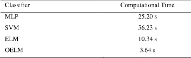
In this section we present our results based on computation complexity and classification rate by comparing the proposed classification technique with other classification techniques using benchmarked EEG datasets. From these by cross fold selection method, we used 50% of the non-overlapped total data for training and remaining 50% of the non-overlapped data for testing. In this work, the Daubechies wavelet of order 2 (db2) made it more appropriate to detect changes of EEG signals since it supports asymmetry and orthogonal. Hence, the wavelet coefficients were computed using the db2 and the number of decomposition levels was chosen to be 4. For implementation of this work we used MATLAB (R2013a) environment running in an Intel Core2 Duo processor with 2.8 GHz. Table IV shows that the computation complexity of OELM is superior to other standard classifiers such as MLP, SVM and ELM. OELM model consumes much lesser
CPU time than SVM, MLP and ELM for unknown samples which shows the greatest advantage of OELM.
TABLE IV
COMPARISON OF VARIOUS CLASSIFICATION METHODS BASED ON COMPUTATIONAL TIME
Classifier Computational Time
MLP 25.20 s
SVM 56.23 s
ELM 10.34 s
OELM 3.64 s
TABLE V
COMPARISON OF VARIOUS CLASSIFICATION METHODS BASED ON CLASSIFICATION RATe
Classifier OELM MLP SVM ELM
Overall
Classification
Accuracy
96% 88% 90% 91%
TABLE VI
COMPARISON OELM CLASSIFICATION ACCURACY BASED ON VARIOUS KERNELs
Kernel Classification Accuracy
Linear 85%
Sigmoid 86%
Gaussian 89%
Linear+Sigmoid 91%
Linear+Gaussian 92%
Linear+Sigmoid+Gaussian 96%
The classification results presented in Table V prove that the OELM with Wavelet features obtains the highest classification accuracy when compared to the other classifiers. Wavelet transform is an effective tool for analysis of non-stationary signal, such as EEGs. The accuracies obtained by the MLP, ELM, SVM are slightly lower than the accuracies of the OELM. And also we compare the OELM classification accuracies by varying the kernels. Table VI presents the classification accuracy of OELM with various kernels. A satisfactory classification accuracy of 96% is achieved in classifying the epileptic EEG signals while using the combination of linear, sigmoid and Gaussian kernels. The accuracy of the ELM can be problematic in many cases, while the OELM remains robust to all tested data sets.
TABLE VII
CLASSIFICATION ACCURACY OFOELM VERSUS OTHER EXISTING CLASSIFIERS
Classifiers Classification Accuracy (%)
OELM (Our work) 94
ELM 92
SVM 90
SLFN 90
TABLE VIII
VALUES OF THE STATISTICAL PARAMETERS OF THE PROPOSED OELM CLASSIFIER FOR VARIOUS EEGDATASET
Dataset Sensitivity (%) Specificity (%) Overall CA (%)
Set A 93.25 98.42
93.63
Set B 93.63 98.36
Set C 94.00 98.16
Set D 94.13 97.17
Set E 93.13 99.54
Table X summarizes classification accuracy and Execution time of various kernels. It is proved that the computation time for ELM kernel is much lesser than other kernels with comparable classification accuracy. Using RBF kernels, the accuracy increases, reaches its maximum and then decreases. In contrast, the accuracy with ELM kernels quickly stabilizes for each dataset. In this work we have considered a complete five classes {ABCDE} of EEG for the classification. In our proposed OELM classifier the computational complexity is lesser when compared with other existing classifiers that are N-1 where N is the number of classes. The efficiency gained in testing phase is very important for many practical applications since the classification stage in application such as epileptic seizure detection is required to be online and requires fast response.
TABLE IX
CLASSIFICATION ACCURACIES AND NUMBER OF CLASSIFIERS REQUIRED
Classifier Classification Accuracy (%)
No. of classier required for N class
problem OELM
(Proposed Work)
94 N
ELM 93
N(N-1)
SVM 90
SLFN 89 N(N-1)
TABLE X
CLASSIFICATION ACCURACY AND EXECUTION TIME VERSUS VARIOUS KERNELS
SVM Kernel Classification Accuracy (%)
Execution time (Seconds)
ERBF 94 24
RBF 91 56
Poly 87 32
Linear 82 25
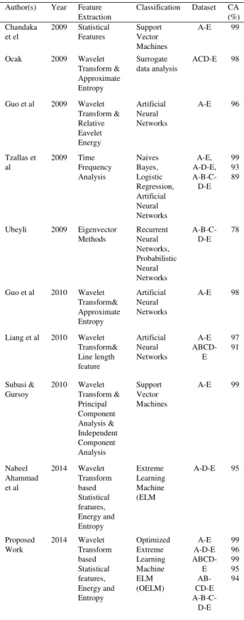
Table XI presents a comparison between our approach and other existing research works. We have used complete 5 classes EEG dataset which are more challenging to classify. Most of the exiting researchers have used only 2 class or 3 class problems. Only a few research works have
used the 5 classes dataset. The proposed OELM with RBF kernel and the features of wavelet transform based statistical coefficients and approximate entropy were used in our work to classify the EEG signals indicated higher performance than that of the other existing research works.
TABLE XI
COMPARISON OF CLASSIFICATION ACCURACY OF THE PROPOSED RESEARCH WORK WITH EXISTING RESEARCH WORKS
Author(s) Year Feature Extraction
Classification Dataset CA (%) Chandaka
et el
2009 Statistical Features
Support Vector Machines
A-E 99
Ocak 2009 Wavelet Transform & Approximate Entropy
Surrogate data analysis
ACD-E 98
Guo et al 2009 Wavelet Transform & Relative Eavelet Energy Artificial Neural Networks
A-E 96
Tzallas et al
2009 Time Frequency Analysis Naives Bayes, Logistic Regression, Artificial Neural Networks A-E, A-D-E, A-B-C-D-E 99 93 89
Ubeyli 2009 Eigenvector Methods Recurrent Neural Networks, Probabilistic Neural Networks A-B-C-D-E 78
Guo et al 2010 Wavelet Transform& Approximate Entropy Artificial Neural Networks
A-E 98
Liang et al 2010 Wavelet Transform& Line length feature Artificial Neural Networks A-E ABCD-E 97 91 Subasi & Gursoy
2010 Wavelet Transform & Principal Component Analysis & Independent Component Analysis Support Vector Machines
A-E 99
Nabeel Ahammad et al
2014 Wavelet Transform based Statistical features, Energy and Entropy Extreme Learning Machine (ELM
A-D-E 95
Proposed Work
V. CONCLUSION
In this paper, an epileptic EEG signal classification system using OELM is proposed and applied to benchmark EEG dataset. The Wavelet based statistical features have been used for the feature extraction. The OELM methodology has been detailed through the presentation in three steps: the plain original ELM as the first step to build the SLFN, followed by a ranking of the neurons by the MRSR algorithm, and finally, the selection of the neurons that will remain. By the use of these steps, the speed and accuracy of the OELM methodology has been demonstrated. We have compared OELM with other traditional classifiers in terms of classification accuracy and computation complexity by evaluating with benchmark EEG dataset. From the obtained experimental results, it can be strongly recommended to use the OELM approach for classifying EEG signals on account of their superior generalization capability as compared to traditional classification techniques. This capability generally provides them with higher classification accuracies and a lower computation complexity. It is a novel, fast and accurate methodology that can be applied to several regression and classification problems. It is found that the performance of the OELM is better in terms of training time and classification accuracy which achieves a satisfying classification accuracy of 96.5% for classifying the epileptic EEG signals. For further work, the comparisons with other methodologies are performed in order to verify the applicability and accuracy of the OELM with different datasets.
ACKNOWLEDGMENT
The authors wish to thank Andrzejak et al., 2001 for the
benchmark EEG dataset available:
(http://www.meb.unibonn.de/epileptologie/science/physik/e egdata.html).
REFERENCES
[1] Y. U. Khan, O. Farooq, and P. Sharma, “Automatic detection of seizure onset in pediatric EEG,” International Journal of Embedded Systems and Applications, vol. 2, no. 3, pp. 81–89, 2012.
[2] E. D. Ubeyli, “Statistics over features: EEG signals analysis,” Computers in Biology and Medicine, vol. 39, no. 8, pp. 733–741, 2009.
[3] H. Adeli, Z. Zhou, and N. Dadmehr, “Analysis of EEG records in an epileptic patient using wavelet transform,” Journal of Neuroscience Methods, vol. 123, no. 1, pp. 69–87, 2003.
[4] S. Sanei and J. A. Chambers, EEG Signal Processing, Centre of Digital Signal Processing, Cardiff University, Cardiff, UK, 2007. [5] J. Gotman, “Automatic recognition of epileptic seizures in the EEG,”
Electroencephalography and Clinical Neurophysiology, vol. 54, no. 5, pp. 530–540, 1982.
[6] Shoeb and J. Guttag, “Application of machine learning to epileptic seizure detection,” in Proceedings of the 27th International Conference on Machine Learning (ICML ’10), pp. 975–982, Haifa, Israel, June 2010.
[7] Sivasankari and K. Thanushkodi, “Automated epileptic seizure detection in EEG signals using FastICA and neural network,” International Journal of Advances in Soft Computing and Its Applications, vol. 1, no. 2, pp. 91–104, 2009.
[8] E. D. Ubeyli, “Wavelet/mixture of experts network structure for EEG signals classification,” Expert Systems with Applications, vol. 34, no. 3, pp. 1954–1962, 2008.
[9] T. Fathima, M. Bedeeuzzaman, O. Farooq, and Y. U. Khan, “Wavelet based feature for Epileptic Seizure Detection,” MES Journal of Technology and Management, vol. 2, no. 1, pp. 108–112, 2011.
[10] I. Daubechies, “Wavelet transform, time-frequency localization and signal analysis,” IEEE Transactions on Information Theory, vol. 36, no. 5, pp. 961–1005, 1990.
[11] T. Gandhi, B. K. Panigrahi, M. Bhatia, and S. Anand, “Expert model for detection of epileptic activity in EEG signature, ”Expert Systems with Applications, vol. 37, no. 4, pp. 3513–3520, 2010.
[12] [E. D. ¨ Ubeyli, “Combined neural network model employing wavelet coefficients for EEG signals classification,” Digital Signal Processing, vol. 19, no. 2, pp. 297–308, 2009.
[13] H. Qu and J. Gotham, “A patient-specific algorithm for the detection of seizure onset in long- term EEG monitoring: possible use as a warning device,” IEEE Transactions on Biomedical Engineering, vol. 44, no. 2, pp. 115–122, 1997.
[14] K. C. Chua, V. Chandran, R. Aeharya, and C. M. Lim, “Higher order spectral (HOS) analysis of epileptic EEG signals,” in Proceedings of the 29thAnnual International Conference of IEEEEMBS, Engineering in Medicine and Biology Society (EMBC ’07), pp. 6495–6498, August 2007.
[15] I. Yaylali, H. Koc¸ak, and P. Jayakar, “Detection of seizures from small samples using nonlinear dynamic system theory,” IEEE Transactions on Biomedical Engineering, vol. 43, no. 7, pp. 743–751, 1996.
[16] M.Niknazar, S. R.Mousavi, B.Vosoughi Vahdat,M. B. Shamsollahi, and M. Sayyah, “A new dissimilarity index of EEG signals for epileptic seizure detection,” in Proceedings of the 4th International Symposium on Communications, Control, and Signal Processing (ISCCSP ’10), Limassol, Cyprus, March 2010.
[17] Y. U. Khan and J. Gotman, “Wavelet based automatic seizure detection in intracerebral electroencephalogram,” Clinical Neurophysiology, vol. 114, no. 5, pp. 898–908, 2003.
[18] M. K. Kiymik, I. G¨uler, A. Dizib¨uy¨uk, and M. Akin, “Comparison of STFT and wavelet transform methods in determining epileptic seizure activity in EEG signals for real-time application,” Computers in Biology andMedicine, vol. 35, no. 7, pp. 603–616, 2005. [19] T. L. Sorensen, U. L. Olsen, I. Conradsen et al., “Automatic epileptic
seizure onset detection usingMatching Pursuit: a case study,” in Proceedings of the Annual International Conference of the IEEE Engineering in Medicine and Biology Society (EMBC ’10), pp. 3277– 3280, 2010.
[20] R. Sukanesh and R. Harikumar, "A Patient Specific Neural Networks (MLP) for Optimization of Fuzzy Outputs in Classification of Epilepsy Risk Levels from EEG Signals," Engineering Letters, 13(2), 50-56, 2006.
[21] .M.J. Er, L.Y. Zhai, X. Li and L. San, "Hybrid Online Sequential Extreme Learning Machine with Simplified Hidden Network," IAENG International Journal of Computer Science, 39:1, pp. 1-9, 2012.
[22] Hong Zhang, "An Analysis of Multiple Particle Swarm Optimizers with Inertia Weight for Multi-objective Optimization," IAENG International Journal of Computer Science, 39:2, pp. 190-199, 2012. [23] H. J. Rong, Y. S. Ong, A. H. Tan and Z. Zhu, "A fast pruned extreme
learning machine for classification problem", Neurocomputing, 72:359-366, 2006.
[24] Gaurang Panchal, Amit Ganatra, Y. P. Kosta and Devyani Panchal, "Behaviour Analysis of Multilayer Perceptrons with Multiple Hidden Neurons and Hidden Layers, International Journal of Computer Theory and Engineering, "Vol. 3, No. 2, ISSN: 1793-8201, 2011. [25] Ingrid Nurtanio, Eha Renwi Astuti, Ketut Eddy Purnama, Mochamad
Hariadi, Mauridhi Hery Purnomo, "Classifying Cyst and Tumor Lesion Using Support Vector Machine Based on Dental Panoramic Images Texture Features," IAENG International Journal of Computer Science, 40:1 pp. 29-37, 2013.
[26] R. Sukanesh, and R. Harikumar, "Diagnosis and Classification of Epilepsy Risk Levels from EEG Signals Using Fuzzy Aggregation Techniques," Engineering Letters, vol 14, No.1, pp. 90-95, 2007. [27] R. G. Andrzejak, K. Lehnertz, F. Mormann, C. Rieke, P. David, and
C. E. Elger, "Indications of nonlinear deterministic and finite-dimensional structures in time series of brain electrical activity: dependence on recording region and brain state," Physical Review E, vol. 64,no. 6, Article ID061907, pp. 1-8, 2001.