Machine Learning for incomplete data

(1)

CENTRO DE CIˆENCIAS

PROGRAMA DE MESTRADO E DOUTORADO EM CIˆENCIA DA

COMPUTA ¸C ˜AO

MESTRADO ACADÊMICO EM CIÊNCIA DA COMPUTA ¸C ÃO

DIEGO PARENTE PAIVA MESQUITA

MACHINE LEARNING FOR INCOMPLETE DATA

(2)

Disserta¸cão apresentada ao Curso de Mes-trado Acadêmico em Ciência da Computa¸cão do Programa de Mestrado e Doutorado em Ciência da Computa¸cão do Centro de Ciências da Universidade Federal do Ceará, como requisito parcial à obten¸cão do t´ıtulo de mestre em Ciência da Computa¸cão. Área de Concentra¸cão:

Orientador: Prof. Dr. Jo˜ao P. P. Go-mes

(3)

Biblioteca Universitária

Gerada automaticamente pelo módulo Catalog, mediante os dados fornecidos pelo(a) autor(a)

M543m Mesquita, Diego Parente Paiva.

Machine Learning for Incomplete Data / Diego Parente Paiva Mesquita. – 2017. 55 f. : il. color.

Dissertação (mestrado) – Universidade Federal do Ceará, Centro de Ciências, Programa de Pós-Graduação em Ciência da Computação, Fortaleza, 2017.

Orientação: Prof. Dr. João Paulo Pordeus Gomes.

1. Machine Learning. 2. Missing Data. I. Título.

(4)

Disserta¸cão apresentada ao Curso de Mes-trado Acadêmico em Ciência da Computa¸cão do Programa de Mestrado e Doutorado em Ciência da Computa¸cão do Centro de Ciências da Universidade Federal do Ceará, como requisito parcial à obten¸cão do t´ıtulo de mestre em Ciência da Computa¸cão. Área de Concentra¸cão:

Aprovada em:

BANCA EXAMINADORA

Prof. Dr. Jo˜ao P. P. Gomes (Orientador) Universidade Federal do Cear´a (UFC)

Prof. Dr. José Antônio Macêdo Universidade Federal do Ceará (UFC)

Prof. Dr. Alu´ızio F. R. Ara´ujo

Universidade Federal de Pernambuco (UFPE)

(5)

(6)

AGRADECIMENTOS

Como todas as coisas da vida, essa disserta¸cão é uma consequência de vários acasos convenientes. Obrigado à todos que me propiciaram esses acasos. Eu extendo esse agradecimento à todos que passaram pela minha vida, mesmo que de maneira breve.

Obrigado aos meus pais, Moacir e Tˆania, por sempre estarem comigo, me proverem de amor e me suportarem de todas as maneiras imagin´aveis.

Obrigado aos demais parentes, em especial ao meu amado avô Eulálio, que não terá a oportunidade de ler isso.

Obrigado aos meus queridos amigos - em especial Eiji Matsui, Luis Freitas e Rebeca Carneiro -, com os quais continuarei a dividir os bons momentos da vida.

Obrigado aos co-autores e amigos: Jo˜ao Paulo P. Gomes, Amauri H. Souza Jr. e Francesco Corona.

Obrigado `a minha amada Rebeca Marcondes pelo cuidado, carinho e incentivo durante essa fase da minha vida.

Obrigado aos colegas, professores e demais funcion´arios do DC-UFC, que sempre fizeram que eu me sentisse confort´avel e bem-vindo.

(7)

(8)

RESUMO

Métodos baseados em fun¸cões de base (como as fun¸cões sigmoid e a q-Gaussian) e medidas de similaridade (como distâncias ou fun¸cões de kernel) são comuns em Aprendizado de Máquina e áreas correlatas. Comumente, no entanto, esses métodos não são equipados para utilizar dados incompletos de maneira orgânica. Isso pode ser visto como um impedimento, uma vez que dados parcialmente observados são comuns em vários dom´ınios, como aplica¸cões médicas e dados provenientes de sensores.

Nesta disserta¸cão, propomos metodologias para estimar o valor do kernel Gaussiano, da distância Euclidiana , do kernel Epanechnikov e de fun¸cões de base arbitrárias na presen¸ca de vetores possivelmente parcialmente observados. Para obter tais estimativas, os vetores incompletos são tratados como variáveis aleatórias cont´ınuas e, baseado nisso, tomamos o valor esperado da transformada de interesse.

(9)

Methods based on basis functions (such as the sigmoid and q-Gaussian functions) and similarity measures (such as distances or kernel functions) are widely used in machine learning and related fields. These methods often take for granted that data is fully observed and are not equipped to handle incomplete data in an organic manner. This assumption is often flawed, as incomplete data is a fact in various domains such as medical diagnosis and sensor analytics. Therefore, one might find it useful to be able to estimate the value of these functions in the presence of partially observed data.

We propose methodologies to estimate the Gaussian Kernel, the Euclidean Distance, the Epanechnikov kernel and arbitary basis functions in the presence of possibly incomplete feature vectors. To obtain such estimates, the incomplete feature vectors are treated as continuous random variables and, based on that, we take the expected value of the transforms of interest.

(10)

LIST OF TABLES

Table 2 – Overview of the experiments. . . 29

Table 3 – Kernel Estimates using different methods . . . 30

Table 4 – Data sets description . . . 31

Table 5 – Gaussian kernel estimation on real-world data: average RMSE . . . 32

Table 7 – Euclidean distance estimates. . . 36

Table 8 – Euclidean distance estimation on real-world data: average RMSE . . . . 38

Table 10 – Epanechnikov kernel estimates. . . 42

Table 12 – Comparison between Expected Epanechnikov Kernel (EEK) and other methods. . . 44

Table 14 – Sigmoid function estimates. . . 50

Table 15 – q-Gaussian function estimates. . . 50

Table 17 – Comparison between SUnscented Transform (UT) and other methods to compute the sigmoid function on real-world data - RMSE values. . . 51

(11)

CMI Conditional Mean Imputation EEK Expected Epanechnikov Kernel EGK Expected Gaussian Kernel EM Expectation Maximization ESD Expected Square Distance GMM Gaussian Mixture Model

ICkNNI Incomplete-Case k-Nearest-Neighbors Imputation algorithm MAR Missing at Random

MC Monte Carlo

MCAR Missing Completely at Random MNAR Missing Not at Random

RBF Radial Basis Function RMSE Root Mean Square Error

(12)

LIST OF SYMBOLS

µ Mean vector

σ Standard deviation Σ Covariance Matrix X Set of feature vectors

X Feature vector

N (Multivariate) Normal p.d.f.

E _{Expected value} Cov Covariance Var Variance

Γ Incomplete Gamma Function

fσ Sigmoid function

k Kernel function k · k2 _{Euclidean norm} G q-Gaussian function

eq q-exponential function exp Exponential

M set of missing entries

O set of observed entries

(13)

1 INTRODUCTION . . . 14

1.1 Objectives and chapters organization . . . 15

1.2 Publications . . . 15

1.2.1 Directly related publications . . . 16

1.2.2 Other contributions . . . 17

2 THEORETICAL BACKGROUND . . . 19

2.1 Missing Data Terminology . . . 19

2.2 Modelling data using GMMs . . . 19

2.3 Expectation Maximization (EM) for Gaussian Mixture Model (GMM)s with Incomplete Data . . . 21

2.4 Imputation Methods . . . 23

2.4.1 Conditional Mean Imputation . . . 23

2.4.2 Incomplete-case K-NN Imputation . . . 24

3 EXPECTED GAUSSIAN KERNEL . . . 25

3.1 Formulation . . . 25

3.2 Experiments and Results . . . 28

3.2.1 EX1: Univariate Normal data with known parameters . . . . 30

3.2.2 EX2: Experiments on Real-World Data . . . 31

3.3 Conclusion . . . 33

4 EXPECTED EUCLIDEAN DISTANCE . . . 34

5 EPANECHNIKOV KERNEL . . . 40

(14)

6 EXPECTED VALUE OF BASIS FUNCTIONS . . . 45

6.1.1 Sigmoid Function. . . 47

6.1.2 q-Gaussian Function . . . 48

7 CONCLUDING REMARKS . . . 53

(15)

1 INTRODUCTION

Data completeness is a major assumption of most Machine Learning methods. In real world problems, however, several data instances may suffer from unobserved/missing attributes. This issue, referred to as missing/incomplete data problem, may happen due to a variety of reasons such as sensor problems, device malfunction and operator mistakes (EIROLA et al., 2014). The simplest way to deal with missing data consists of removing the instances with missing attributes (listwise deletion) from the dataset. Even though this approach may work in some cases, discarding data samples usually leads to loss of important information to build a learning model (EIROLA et al., 2013). Another widely used approach is to perform a pre-processing step of missing data imputation. After filling the missing entries, any conventional learning method can be used. Examples of such an approach can be found in (KANG, 2013), (LOBATO et al., 2015), (ASTE et al., 2015) and (GHEYAS; SMITH, 2010).

According to Acu˜na and Rodrigues in (ACU ˜NA; RODRIGUEZ, 2004), problems with more than 5% of missing samples may require sophisticated handling methods. In such situations, good results can be achieved by not considering the imputation as a separate step. Rather, it is possible to design a learning method that can handle incomplete data in its formulation. By doing so, the inherent uncertainty of the imputation process is taken into account and it has shown to be beneficial in many cases (SOVILJ et al., 2016). On the other hand, direct imputation omits this uncertainty, which might be prejudicial depending on the context.

For example, let Xi = (xi,1, . . . , xi,D)T and Xj = (xj,1, . . . , xj,D)T be two (independent) possibly incomplete feature vectors. Suppose we are interested in estimating the squared Euclidean distance _kXi−Xjk2 between these vectors, which is an important piece in many Machine Learning methods, such as Nearest Neighbors methods andk-means. Treating the missing entries as independent random variables, according to Eirola et al.

(2013), the desired expected value can be expressed as:

E_[_k_X_i₋_X_j_k2_{] =} D X

d=1

(E_[_x_i,d]₋E_[_x_j,d])2_{+ Var[}_x_{i,d] + Var[}_x_j,d]_,

(16)

15

lead to:

kE_[_X_i_]₋E_[_X_j_]_k2 ₌ D X

d=1

(E_[_x_i,d_]₋E_[_x_j,d_])2_,

which ignores the variances respective to the missing entries and, depending on their magnitude, might grossly diverge from E_[_k_X_i ₋_X_j_k2_].

In this work, we provide tools to directly estimate transforms of incomplete feature vectors, in the a similar fashion to what (EIROLA et al., 2013) proposed for the squared Euclidean distance.

1.1 Objectives and chapters organization

The general objective of this work is to provide tools for adapting Machine Learning methods which incorporate the uncertainty arising form the imputation process, similarly to what was presented in (EIROLA et al., 2013) and Eirolaet al. (2014) for the squared Euclidean distance. We present these in the form of methodologies to estimate transforms of the values which would be otherwise imputed. As specific objectives, we address the problems of estimating:

1. the Gaussian Kernel between two possibly incomplete feature vectors; 2. the Euclidean Distance between two possibly incomplete feature vectors; 3. the Epanechnikov Kernel between two possibly incomplete feature vectors; 4. the value of basis functions applied to a possibly incomplete feature vector.

A theoretical background covering basic concepts and commonly used imputa-tion methods is provided in chapter 2. Soluimputa-tions to the aforemenimputa-tioned specific objectives are presented, in order, in chapters 3, 4 and 5. In chapter 7, we provide final reflections on the content of the presented work and discuss directions for future works.

1.2 Publications

(17)

1.2.1 Directly related publications

1. Diego P. P. Mesquita, Jo˜ao P. P. Gomes, Amauri H. Souza Junior Epanechnikov Kernel for Incomplete Data

Electronics Letters, 2017.

2. Diego P. P. Mesquita, Jo˜ao P. P. Gomes, Amauri H. Souza Junior, Juvˆencio S. Nobre Euclidean Distance Estimation in Incomplete Datasets

Neurocomputing, 2017.

3. Marcelo B. Veras, Diego P. P. Mesquita, Jo˜ao P. P. Gomes, Amauri H. Souza Junior, Guilherme A. Barreto

Forward Stagewise Regression on Incomplete datasets

International Work-conference on Aritifical Neural Networks, 2017. 4. Diego P. P. Mesquita, Jo˜ao P. P. Gomes, Leonardo R. Rodrigues

K-means for Datasets with Missing Attributes: Building Soft Constraints with Observed and Imputed Values

European Symposium on Artificial Neural Networks, 2016.

5. Diego P. P. Mesquita, Jo˜ao P. P. Gomes, Leonardo R. Rodrigues

Extreme Learning Machines for Datasets with Missing Values Using the Unscented Transform

Brazilian Conference on Intelligent Systems, 2016 . 6. Diego P. P. Mesquita, Jo˜ao P. P. Gomes

Radial Basis Function Neural Networks for datasets with missing values

International Conference on Intelligent Systems Design and Applications, 2016 . 7. Diego P. P. Mesquita, Jo˜ao P. P. Gomes, Amauri H. Souza Junior A Minimal

Learning Machine for datasets with missing values

International Conference on Neural Information Processing, 2015.

8. Diego P. P. Mesquita, Jo˜ao P. P. Gomes, Francesco Corona, Amauri H. Souza Junior, Juvˆencio S. Nobre

Gaussian Kernels for Incomplete Data

(18)

17

1.2.2 Other contributions

1. Diego P. P. Mesquita, Jo˜ao P. P. Gomes, Leonardo R. Rodrigues, Saulo A. F. Oliveira and Roberto K. H. Galv˜ao

Building Selective Ensembles of Randomization Based Neural Networks with the Successive Projections Algorithm

Applied Soft Computing, 2017.

2. Diego P. P. Mesquita, Jo˜ao P. P. Gomes, Amauri H. Souza Junior

Ensemble of Efficient Minimal Learning Machines for Classification and Regression

Neural Processing Letters, 2017.

3. Diego P. P. Mesquita, Lincoln S. Rocha, Jo˜ao P. P. Gomes, Ajalmar R. Rocha Neto Classification with Reject Option for Software Defect Prediction

Applied Soft Computing, 2016.

4. Diego P. P. Mesquita, Jo˜ao P. P. Gomes, Leonardo R. Rodrigues, Roberto K. H. Galv˜ao

Pruning Extreme Learning Machines Using the Successive Projections Algorithm

IEEE Latin America Transactions, 2015.

5. Jo˜ao P. P. Gomes, Diego P. P. Mesquita, Ananda L. Freire, Amauri H. Souza Junior, Tommi Karkkainen

A Robust Minimal Learning Machine based on the M-Estimator

6. Diego P. P. Mesquita, Antônio N. Araújo Neto, José F. Queiroz Neto, João P. P. Gomes, Leonardo R. Rodrigues

Using Robust Extreme Learning Machines to Predict Cotton Yarn Strength and Hairiness

7. Filipe F. R. Damasceno, Diego P. P. Mesquita, Marcelo B. Veras, Jo˜ao P. P. Gomes, Carlos E. F. de Brito

Shrinkage k-means: A clustering algorithm based on the James-Stein Estimator

(19)

8. Weslley L. Caldas, Michelle G. Cacais, Jo˜ao P. P. Gomes, Diego P. P. Mesquita Co-MLM: a SSL algorithm based on the Minimal Learning Machine

Brazilian Conference on Intelligent Systems, 2016 .

9. Diego P. P. Mesquita, Jo˜ao P. P. Gomes, Amauri H. Souza Junior, Guilherme A. Barreto

Ensemble of Minimal Learning Machine for Pattern Classification

(20)

19

2 THEORETICAL BACKGROUND

In this chapter, we introduce some basic concepts which might be useful to understanding the developments presented in the next chapters. In Section 2.1, we introduce basic missing data concepts regarding the processes which causes entries to be missing. In Section 2.2, we introduce the Gaussian Mixture Model (GMM) and address how to use it to obtain statistics of missing components in a vector. In Section 2.3, we introduce Expectation Maximization (EM) as a procedure to estimate the parameters of a GMM from incomplete datasets. Finally, in Section 2.4, we give an overview of two popular imputation strategies that will be used for comparison.

2.1 Missing Data Terminology

Consider a D-dimensional random vector X with observed entries indexed as

XO and missing ones as XM. Let I ∈ {0,1}D be an indicator vector such that the In equals one if and only if Xn is observed, i.e., n∈O. We say data is Missing Completely at Random (MCAR) if the probability an entry is missing in X is independent of values of both the observed and missing entries of X, which can be expressed as:

P(I|XO, XM) =P(I).

Differently from MCAR, data is said to be Missing at Random (MAR) when the probability that a component Xn of X is missing is independent of its true (unknown) value, but might depend of XO. This can be expressed as:

P(I_|XO, XM) =P(I|XO)

When the probability that an entry is missing is intrinsically related to its value, it is said that data is Missing Not at Random (MNAR). In this work, we consider data is MAR. A more comprehensive account of missing data mechanisms can be found in Molenberghs et al. (2014).

2.2 Modelling data using GMMs

To provide a flexible representation for the distribution from which the feature vectors in a dataset _X =_{X_n}N

(21)

linear superposition of C D-dimensional Gaussian densities, each with its own meanµ(c) and covariance matrix Σ(c)_{, with} _c _{= 1}_{, . . . , C}_{, i.e., a Gaussian Mixture Model (GMM)} . Given an arbitrary Xn ∈ RD, the probability density function of a GMM (HUNT; JORGENSEN, 2003) with the aforementioned parameters takes the form:

p(Xn) = C X

c=1

w(c)N(Xn|µ(c),Σ(c)), (2.1)

where _{w(c)_}C

c=1 is a set of non-negative scalars that satisfy the convexity constraint PC

c=1w(c) = 1. The GMM model is a flexible and powerful modeling tool capable to model a wide class of continuous distributions, provided a sufficient number of Gaussian components.

It is instrumental for the developments in this work to be able to obtain estimates of the non-central moments of the missing entries of a feature vector. It is known that, for a single Gaussian (C = 1) these moments can be expressed as functions of its mean vector and covariance matrix. In turn, the mean and covariance of the missing entries can be computed by conditioning the Gaussian on the observed entries of the vector. In a GMM, the moments are given by a weighted sum of the moments of the Gaussian components.

For instance, consider an arbitrary vector Xn, with missing component values

Xn,M and observed component values Xn,O, whereM and O denote the sets of indexes of missing and observed component values, respectively. Then, the parameters µ(c) _{and Σ}(c) of the c-th component of the GMM can be partitioned into blocks as follows:

µ(c) =  

µ(_Oc) µ(_Mc)



, Σ(c)=  

Σ(_OOc) Σ(_OMc) Σ(_{M O}c) Σ(_{M M}c)



. (2.2)

Then, the mean vector ˜µ(nc) = E(c)[Xn,M|Xn,O] and covariance matrix ˜Σ(nc) = Var(c)[Xn,M|Xn,O] of the c-th Gaussian in the GMM, conditioned on Xn,O, are given by

˜

µ_n(c) =µ(_Mc)+ Σ(_{M O}c) (Σ_OO(c))−1(Xn,O−µ(Oc)), (2.3) ˜

Σ(_nc) = Σ(_{M M}c) −Σ_{M O}(c) (Σ(_OOc))−1Σ(_OMc) , (2.4)

(22)

21

by

E[xn,d] = C X

c=1

w(c)µ˜(_n,dc), (2.5)

E[x2_n,d] = C X

c=1

w(c)[˜µ(_n,dc)]2+ ˜Σ(_n,dc), (2.6)

E[x3n,d] = C X

c=1

w(c)[˜µ(_n,dc)]3+ 3˜µ(_n,dc)Σ˜(_n,dc), (2.7)

E[x4_n,d] = C X

c=1

w(c)[˜µ_n,d(c)]4+ 6[˜µ(_n,dc)]2Σ˜(_n,dc) + 3[ ˜Σ_n,d(c)]2, (2.8)

in which ˜µ(_n,dc) denotes the d-th element of vector ˜µn(c) and ˜Σ(_n,dp) denotes the d-th element along the main diagonal of matrix ˜Σ(np).

2.3 EM for GMMs with Incomplete Data

Expectation-maximization algorithms are efficient approaches for finding a maximum likelihood solution for models with latent variables as a Gaussian mixture model, without relying on iterative numerical optimization techniques. Given a likelihood function of some parameters, EM algorithms consist of two steps, an expectation and a maximization step: In the first step, the expected value of some latent variables is taken; in the latter, the most likely estimates for the parameters are computed. The two steps are repeated until convergence of either the parameters or the likelihood. We briefly overview the EM algorithm for GMMs with complete data and its extension for incomplete data (HUNT; JORGENSEN, 2003).

Consider a data set X = {Xn}N

n=1 comprising N samples and the Gaus-sian mixture distribution p(Xn) = PC_c₌₁w(c)_N₍_X

n|µ(c),Σ(c)) consisting of C densities N(Xn|µ(c)_,_Σ(c)_{). Let Θ =} _{_w(c)_{, µ}(c)_,_Σ(c)_}C

c=1 with w(c) as mixing coefficient of the c-th Gaussian and µ(c) _{and Σ}(c) _{its mean vector and covariance matrix. We want to maximize} the likelihood LX(Θ) of the parameters Θ

LX(Θ) =

N Y n=1 C X c=1

w(c)_N₍_X_n|_µ(c)_,_Σ(c)₎ !

. (2.9)

(23)

1. The expectation (E) step computes the expected memberships tn,c of each sample n

tn,c=

w(c)_N₍_X

n|µ(c),Σ(c)) P

lw(l)N(Xn|µ(l),Σ(l))

, (2.10)

with respect to each Gaussian c= 1, . . . , C.

2. The maximization (M) step consists of computing the most likely estimates for the parameters in Θ

µ(c)= 1

Nc N X n=1

tn,cXn, (2.11)

Σ(c)= 1

Nc N X n=1

tn,c(Xn−µ(c))(Xn−µ(c))T, (2.12)

w(c)= Nc

N . (2.13)

with Nc =PN_n₌₁tn,c and for c= 1, . . . , C.

Although the formulation is a well-established approach to fit Gaussian mixture models to complete data, a number of modifications are required to extend it to the case of incomplete data. The idea consists in treating missing values as latent variables to be estimated in the expectation step. The likelihood given the observed values takes the form

LX(Θ) =

N Y n=1 C X c=1

w(c)_N(Xn,O|µ(Oc),Σ (c) OO)

!

, (2.14)

where Xn,O denotes the observed entries of Xn and {µ(Oc),Σ (p) OO}C

c=1 are the parameters of the c-th Gaussian when marginalizing on the observed entries of Xn.

To make use of the marginal probability on the observed entries, the E-step in Eq. (2.10) is modified to yield

tn,c=

w(c)_N₍_X_n,O|_µ(c) O ,Σ

(c) OO) P

lw(l)N(Xn,O|µ (l) O,Σ

(l) OO)

. (2.15)

The E-step is further augmented with the following equations that compute the parameters _{µ˜(nc),Σ˜n(c)}Cc=1 of the distribution of the missing entries Xn,M conditioned on Xn,O, i.e ˜µ(nc) = E(c)[Xn,M|Xn,O] and ˜Σ(nc) = Var(c)[Xn,M|Xn,O]. For each Gaussian:

˜

µ_n(c) = µ(_n,Mc) + Σ(_{M O}c) (Σ_OO(c))−1(Xn,O−µ(n,Oc) ), ˜

(24)

23

As for the M-step, Eq. (2.13) that computes the weights of the mixture remains functionally unaltered, while Eqs. (2.11) and (2.12) are modified to yield

µ(c) = 1

Nc N X n=1

tn,cX˜n(c),

Σ(c) = 1

Nc N X n=1

tn,c( ˜X_n(c)−µ(c))( ˜X_n(c)−µ(c))T + N X n=1

tn,cΣ(_nc),

where:

˜

X_n(c)=  

Xn,O ˜

µ(nc) 

, Σ(_nc) =  

0OO 0OM 0M O Σ˜(nc)



. (2.16)

In other words, ˜Xn(c) denotes the vector Xn imputed with ˜µ(nc) on its missing entries and Σ(nc) is the conditional covariance matrix ˜Σ(nc) padded with zeros.

2.4 Imputation Methods

2.4.1 Conditional Mean Imputation

Conditional Mean Imputation (CMI) consists in estimating a probability distri-bution for the missing entries in a vector and using its mean value to fill the entries. The usual approach to obtain such distribution is to first obtain a model for the distribution from which the feature vectors of the dataset were drawn and then condition on the observed values of each incomplete vector.

Letpdenote the probability density function obtained from a datasetX . Given an incomplete vector X _{∈ X}, CMI consists in filling each missing entry xi,k of X with:

Z ∞

−∞

φp(φ|xi,O)dφ (2.17)

wherep(_·|xi,O) denotes the p.d.f. p conditioned on the observed entries of X.

For the case in which p is the p.d.f. of a Gaussian distribution, so is the conditional p(_·|xi,O), which can be obtained as described in Section 2.2. If the parameters of p(·|xi,O) areµ (mean vector) and Σ (covariance matrix), Eq. 2.17 resumes toµ.

(25)

2.4.2 Incomplete-case K-NN Imputation

Incomplete-case k Nearest Neighbors imputation (ICkNNI) is a non-parametric distance-based imputation method recently proposed by Hulse e Khoshgoftaar (2014). The idea behind ICkNNI is to use the incomplete Euclidean distance in order to select the k

nearest fully observed neighbors for each incomplete feature vector, then filling the missing entries with the average of the selected neighbors. In this Section , we provide a review of ICkNNI.

Consider a set _X =_{Xn}Nn=1 comprising both complete and incomplete feature vectors. Let xi,k denote the k-th component of Xi and Oi be the set of indices of the observed entries in Xi. Furthermore, let

N_i,j ₌_{_X_n_{∈ X |}_O_i_{∪ {}_j_{} ⊆}_O_n} _(2.18)

be the set of points in _X which count on all the observed features of Xi plus feature

j ∈Mi.

The incomplete euclidean distance d can be defined as:

d(Xi, Xj) =     

q P

k∈Oi(xi,k−xj,k)

2_, _if _O

i ⊆Oj;

∞, otherwise.

(2.19)

In Incomplete-Case k-Nearest-Neighbors Imputation algorithm (ICkNNI), for each incomplete feature vector Xi ∈ X, andl ∈Oi, we construct the set Ci,j consisting of the k nearest neighbors of Xi in the set Ni,j according to d(Xi,·). Then we fill the missing component xi,j with:

X Xj∈Ci,j

xj,l

(26)

25

3 EXPECTED GAUSSIAN KERNEL

The Gaussian Kernel, often referred to as the Radial Basis Function (Radial Basis Function (RBF)) kernel is one of the most common kernels in Machine Learning, finding application in various methods, such as Support Vector Machines, Gaussian Processes and RBF networks.

Given twoD-dimensional vectorsXi = (xi,1, . . . , xi,D)T andXj = (xj,1, . . . , xj,D)T, the Gaussian kernel is given by

k(Xi, Xj),exp (

−kXi−Xjk 2 2σ2

)

, (3.1)

where σ2 _> _{0 is the scale hyper-parameter and} _k_X

i−Xjk2 =PDd=1(xi,d−xj,d)2, i.e., k · k denotes the L2 norm.

In this Chapter, we present a methodology to estimate k(Xi, Xj) when vectors

Xi, Xj ∈ X count on one or more missing components.

3.1 Formulation

Let Xi and Xj be two possibly partially observed feature vectors drawn from a same distribution and let z =_kXi −Xjk2. Note z is a random variable as it is a tranform of the missing entries of Xi and Xj. In turn, so isk(Xi, Xj), since it can be written as:

k(Xi, Xj) = exp (

− z 2σ2

)

. (3.2)

Thus, estimating k(Xi, Xj) comes down to computing:

E_[_k₍_X_i_{, X}_{j)] =} E "

exp (

− ₂z_σ₂ )# = Z ∞ −∞ exp (

−₂z_σ₂ )

pz(z)dz (3.3)

wherepz denotes the probability density function ofz. Furthermore, asz is non-negative:

E_[_k₍_X_i_{, X}_j_{)] =} Z ∞

0 exp

( − z

2σ2 )

pz(z)dz = Z

(0,∞) exp

( − z

2σ2 )

pz(z)dz. (3.4)

Recall the definition of the moment-generating functionMzof a random variable

z with p.d.f. pz whose support is (0,∞):

Mz(t) = Z

(0,∞)

(27)

hence:

E_[_k₍_X_i_{, X}_j_{)] =} _M_z ₋ 1 2σ2

!

, (3.6)

i.e., computingE_[_k₍_X_i_{, X}_{j)] boils down to evaluating} _M_z₍_·_{) at} _t₌₋₁_/₍₂_σ2_{). For such, we} need to choose a distribution for z.

For d = 1. . . D, letφ2

d= (xi,d−xj,d)2. Consequently, since the differences φd can1 _{be treated as random variables,} _z ₌PD

d=1φ2d is a sum of squared random variables. According to Roberts e Geisser (1966), the distribution of a squared random variableφ2

d is said to be Gamma - with parameters αd and βd - if:

1. the distribution pd of φd can be written as:

pd(φd) =h(φd)_|φ_|2αd−1_exp(₋_β

dφ2d);

2. There exists a constant ζ such that:

∀φd:h(φd) +h(−φd) = ζ.

A variety of different distributions conform to the above conditions. Some examples are the Gaussian distribution, the Skew Normal (AZZALINI, 1985) (which generalizes the Gaussian distribution and allows for non-zero asymmetry), Kotz-type distributions (that are bi-modal and may have light tails) as well as other heavy- and light-tailed distributions obtained similarly to the Skew Normal (ROBERTS; GEISSER, 1966; JOHNSON N.; BALAKRISHNAN, 1995; GENTON, 2004).

It is then reasonable to model z as a sum of Gamma-distributed random variables. Furthermore, Covo e Elalouf (2014) showed the sum of independent Gamma distributed random variables can be well approximated by a Gamma distribution under mild conditions. This independence assumption is satisfied if we assume the missing components of a vector are independent among themselves. This premise can be found in (EIROLAet al., 2013) and (EIROLAet al., 2014), and we take it as well. Thus, we assume

z follows a Gamma distribution with shape and inverse scale parameters, respectively,

α, β >0. Hence, pz(·) is given by:

p(z_|α, β) = β α Γ(α)z

α−1_{exp (}

−βz), (3.7)

1 _{In case both}_x

(28)

27

where Γ(α) =R+∞

0 u

α−1_{exp (}₋_α₎_du _{is the gamma function.}

In particular, for the Gamma distribution, Mz(·) has a closed-form solution:

Mz(t) = 1₋ t

β

!−α

∀t < β, (3.8)

and Eq. (3.6) turns into:

E_[_k₍_X_i_{, X}_j_{)] =} _M_z ₋ 1 2σ2

!

= 2βσ 2 2βσ2_{+ 1}

!α

. (3.9)

To estimate k(Xi, Xj), we still have to estimate the parameters α andβ of the Gamma distribution. These can be obtained via method-of-moments from the mean E_[_z_] and the variance Var[z] of the squared distance z:

α = E_[_z_]2

Var[z], β = E_[_z_]

Var[z]. (3.10)

The problem of estimating E[z] can be approached using the results from (EIROLA et al., 2013) and (EIROLA et al., 2014), in which expected squared distances

are expressed in the form

E[z] = X d /∈Mi∪Mj

(xi,d−xj,d)2+ X d∈Mj\Mi

E[(xi,d−xj,d)2]

+ X

d∈Mi\Mj

E[(xi,d −xj,d)2] + X d∈Mi∩Mj

E[(xi,d−xj,d)2], (3.11)

withMi, Mj ⊆ {1, . . . , D} denoting the sets of indexes of the missing components of Xi and Xj, respectively. Since all of the terms in eq. (3.11) can be expanded to yield:

E_[(_x_i,d₋_x_j,d)2_{] =} E_[_x2

i,d] +E[x2j,d]−2E[xi,d]E[xj,d]

= (

E_[_x2_i,d_]₋E_[_x2_i,d_{] +}E_[_x2_j,d_]₋E_[_x2_j,d_] +E_[_x_i,d_]2₊E_[_x_j,d_]2₋₂E_[_x_i,d_]E_[_x_j,d_] = (E_[_x_i,d]₋E_[_x_j,d])2_{+ Var[}_x_{i,d] + Var[}_x_j,d]_,

the expected squared distance z can be compactly written as

E_[_z_{] =} D X d=1

(29)

Although not derived in (EIROLA et al., 2013) and (EIROLA et al., 2014), analogous reasoning can be used to express the variance of the squared distances Var[z]:

Var[z] = Var " _D

X d=1

(xi,d −xj,d)2 # = D X d=1 Var

(xi,d −xj,d)2 + D X d=1 D X l=d+1

Cov

(xi,d−xj,d)2,(xi,l−xj,l)2

.

(3.13)

Using independence assumptions stated before, Eq. (3.13) reduces to:

Var[z] = D X

d=1 Var

(xi,d −xj,d)2

= D X

d=1

E₍_x_i,d₋_x_j,d)4₋E₍_x_i,d₋_x_j,d)22

=            D X d=1

E_x4

i,d+x4j,d−4x3i,dxj,d−4xi,dx3j,d+ 6x2i,dx2j,d

− D X d=1

E₍_x_i,d₋_x_j,d)22_.

(3.14)

Together, eqs. (3.12) and (3.14) show how the expectation and the variance of squared distances can be expressed only in terms of non-central moments of Xi and Xj. Such moments can be estimated by imposing a distribution from which Xi and Xj are drawn and estimating the parameters of such distribution. Any model-estimation method capable of generating probability distributions for each missing variable can be used for the task.

3.2 Experiments and Results

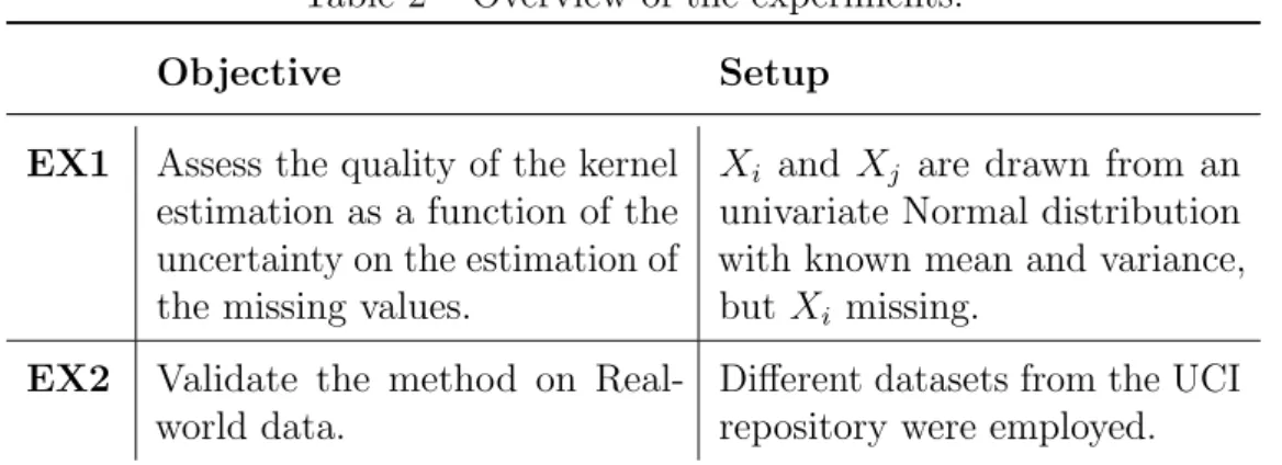
We perform two different experiments to validate our approach, the Expected Gaussian Kernel (EGK) . In the first, we study how the uncertainty on the estimation of the missing values affects the quality of the kernel estimate. In second, we evaluate EGK on real-world data. Table 2 summarizes the details of these experiments.

(30)

29

Table 2 – Overview of the experiments.

Objective Setup

EX1 Assess the quality of the kernel estimation as a function of the uncertainty on the estimation of the missing values.

Xi and Xj are drawn from an univariate Normal distribution with known mean and variance, but Xi missing.

EX2 Validate the method on Real-world data.

Different datasets from the UCI repository were employed.

consists in estimating _kXi −Xjk2 and plugging it into the kernel expression. On the other hand, EGK directly estimates the transform of interest. This conceptual difference between the approaches is condensed in Eqs. (3.15) to (3.17).

ˆ

kEGK(Xi, Xj) = E "

exp (

− kXi −Xjk 2 2σ2

)#

, (3.15)

ˆ

kESD(Xi, Xj) = exp (

−

E_k_X_i₋_X_j_k2 2σ2

)

, (3.16)

ˆ

kCM I(Xi, Xj) = exp (

− k

E_[_X_i]₋E_[_X_j_]_k2 2σ2

)

. (3.17)

It has been pointed out by Eirola et al. (2013) that estimating the missing entries before taking the squared euclidean distance tends to underestimate the expected value of this transform. As a consequence - see Eq. (3.12) -, we have

ˆ

kESD(Xi, Xj)≤kˆCM I(Xi, Xj). (3.18)

Assuming z is Gamma-distributed, a similar statement can be made via direct application of Jensen’s inequality. Recall Jensen’s inequality states that:

g(E_[_φ_])_≤E_[_g₍_φ_)] _(3.19)

for any integrable real-valued random variable φ and convex function g(·). Applying it directly to Eq. (3.15), one can obtain

ˆ

(31)

3.2.1 EX1: Univariate Normal data with known parameters

For this experiment, we fix Xj = 3, assume Xi ∼ N(2, σ2n) and estimate

k(Xi, Xj). Since the distribution of Xi is known, there is no need to estimate a model for the data as the true distribution _N(2, σ2

n) is given. We set the kernel hyper-parameter

σ2 _{= 1.}

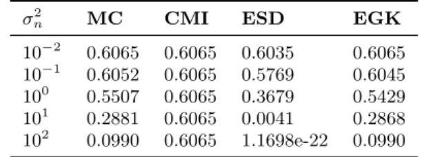
To obtain a benchmark, we compute a Monte Carlo (Monte Carlo (MC)) estimate of k(Xi, Xj) by performing 108 draws of Xi from N(2, σn2), taking the kernel value for each of these draws and then averaging the computed kernel values. Using this procedure, we aim to accurately approximate the expected value the kernel. Based on that, a method is as good as its estimates are similar to the ones obtained by via Monte Carlo. Table 3 compiles the results of the experiments for different values of σ2

n. Table 3 – Kernel Estimates using different methods

σ_n2 MC CMI ESD EGK

10−2 _0.6065 _0.6065 _0.6035 _0.6065

10−1 _0.6052 _0.6065 _0.5769 _0.6045

100

0.5507 0.6065 0.3679 0.5429 101

0.2881 0.6065 0.0041 0.2868 102

0.0990 0.6065 1.1698e-22 0.0990

Note that CMI computes the same approximation regardless of the value of

σ2

n. This is expected, since the the expected value of Xi depends only of µ. While both CMI and ESD quickly deteriorate as σ2

(32)

31

3.2.2 EX2: Experiments on Real-World Data

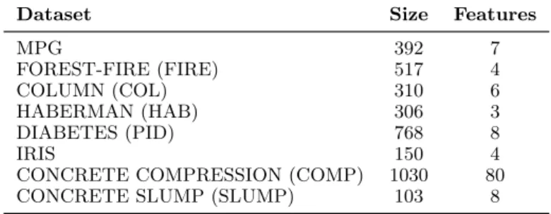
In this second experiment, we evaluate the performance of EGK in real world data sets for different amounts of missing data. All data used for this experiments is available at the UCI repository of Machine Learning data sets (LICHMAN, 2013). Details concerning the number and size of the feature vectors in each of data set can be found in Table 4.

Table 4 – Data sets description

Dataset Size Features

MPG 392 7

FOREST-FIRE (FIRE) 517 4

COLUMN (COL) 310 6

HABERMAN (HAB) 306 3

DIABETES (PID) 768 8

IRIS 150 4

CONCRETE COMPRESSION (COMP) 1030 80 CONCRETE SLUMP (SLUMP) 103 8

Ten similar rounds of experiment were carried. In each of these, the percentage of instances with missing vectors was iteratively increased from 10% to 50% (in steps of 20%) of the dataset size. The number of features to be deleted in each of these vectors is decided independently by drawing a number from {1,· · · ,⌈D/3⌉}. In each step we use different methods to estimate the kernel matrix and measuring the Root Mean Squared-Error between these estimates and the true kernel matrix computed beforehand. In this experiments, the true distribution of the data is unknown, thus, at each step we estimate a GMM comprising three components.

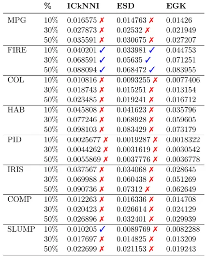
We do not consider CMI in this experiment, as it was consistently outperfor-med by the other methods in the previous experiment. Instead, we substitute it by the Incomplete-Case k-Nearest-Neighbors Imputation algorithm (ICkNNI) (HULSE; KHOSH-GOFTAAR, 2014), a well-known distance-based imputation algorithm that does not rely on the estimation of a statistical model for the data. The parameters for ICkNNI were implemented as suggested in Hulse e Khoshgoftaar (2014). Results, in terms of average Root Mean Square Error (RMSE), are presented in Table 5. We employed Wilcoxon’s signed-rank test, with a 5% significance level, to verify the statistical significance of the results. The symbols ✓_and ✗ _{indicate the result of the hypothesis test (}✓ _{fail to reject,}

and ✗ _reject).

(33)

missing values. Specifically for ESD and EGK, performance deteriorates due to the quality of distribution estimated for the data, which is affected by the amount of missing data.

Again, EGK achieved the best overall results. This fact provides some evidence that the assumptions taken in the formulation of EGK do not affect negatively its per-formance on real world data. Additionally, it is interesting to verify that even using a statistical model with only three Gaussians, EGK was able to outperform a non-parametric model such as the ICkNNI.

Table 5 – Gaussian kernel estimation on real-world data: average RMSE

% ICkNNI ESD EGK

MPG 10% 0.016575✗ 0.014763 ✗ 0.01426 30% 0.027873✗ _0.02532✗ _0.021949

50% 0.035591✗ 0.030675 ✗ 0.027207 FIRE 10% 0.040201✓ 0.033981 ✓ 0.044753 30% 0.068591✓ 0.05635✓ 0.071251 50% 0.088094✓ 0.068472 ✓ 0.083955 COL 10% 0.010816✗ 0.0093255 ✗ 0.0077406

30% 0.018743✗ _0.015251 ✗ _0.013154

50% 0.023485✗ 0.019241 ✗ 0.016712 HAB 10% 0.045808✗ 0.041623 ✗ 0.035796 30% 0.077246✗ 0.068928 ✗ 0.059605 50% 0.098103✗ _0.083429 ✗ _0.073179

PID 10% 0.0025677✗ _0.0019287 ✗ _0.0018322

30% 0.0044262✗ 0.0031619 ✗ 0.0030542 50% 0.0055869✗ 0.0037776 ✗ 0.0036778 IRIS 10% 0.037567✗ 0.034068 ✗ 0.028645

30% 0.069988✗ 0.060438 ✗ 0.051269 50% 0.090736✗ _0.07312✗ _0.062649

COMP 10% 0.012263✗ _0.016336 ✗ _0.014708

30% 0.020423✗ 0.026614 ✗ 0.024129 50% 0.026896✗ 0.032401 ✗ 0.029939 SLUMP 10% 0.010205✓ 0.0089769 ✗ 0.0082288

30% 0.017697✗ _0.014825 ✗ _0.013209

(34)

33

3.3 Conclusion

In this chapter, we presented a methodology to estimate the Gaussian Kernel between two feature vectors Xi and Xj when one or both have missing entries. The proposed method takes the expected value of the kernel k(Xi, Xj) as a transform of the squared Euclidean distancez =kXi−Xjk2. In turn, zis modelled as a Gamma-distributed random variable and a procedure is outlined to compute the parameters that govern this distribution.

(35)

4 EXPECTED EUCLIDEAN DISTANCE

Given twoD-dimensional vectorsXi = (xi,1, . . . , xi,D)T andXj = (xj,1, . . . , xj,D)T, the Euclidean distance η between Xi and Xj is given by

η =z1/2 ,

v u u t

D X d=1

(xi,d−xj,d)2, (4.1)

where, as in the previous Chapter,z denotes the squared distance between Xi and Xj. In this Chapter, we present a methodology to estimateη when vectorsXi, Xj ∈ X count on one or more missing components. Following the developments of the previous chapter, we assume z is a Gamma-distributed random variable.

4.1 Formulation

Note that η is a random variable as it is a non-negative transform of Xi and

Xj. Hence, taking the expected value of η consists in computing:

E_[_η_{] =} Z +∞

0

η p(η) dη. (4.2)

Drawing from the previous chapter, we say z follows a Gamma distribution with parameters α and β that can be estimated from the non-central moments of Xi and

Xj as described bofore. It is then sensible to choose the Nakagami (NAKAGAMI, 1960) distribution for η. By definition, since η is the square-root transform of z:

η ∼Nakagami(m,Ω), (4.3)

where m and Ω are, respectively, the shape and spread parameters of the Nakagami distribution. Under this setup, the expected value of η is given by:

E_[_η_{] =} Γ(m+ 1 2) Γ(m)

Ω

m

!12

. (4.4)

In turn, using the method-of-moments, the parameters mand Ω can be written as functions of the mean and variance of z according to:

m = E

2_[_z_]

Var[z], Ω =E[z]. (4.5)

(36)

35

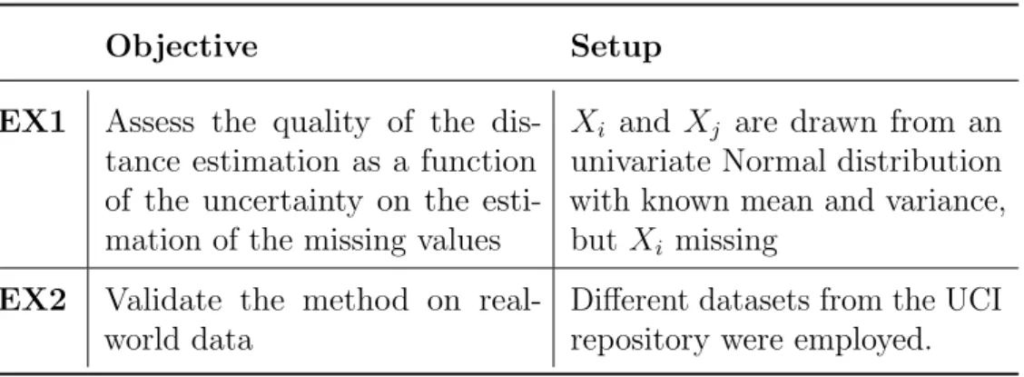
We perform two different experiments to validate our methodology (EED) . In the first, we study how the uncertainty on the estimation of the missing values affects the quality of the distance estimate. In second, we evaluate EED on real-world data. Table 6 summarizes the details of these experiments. The following subsections present and discuss the results.

Objective Setup

EX1 Assess the quality of the dis-tance estimation as a function of the uncertainty on the esti-mation of the missing values

Xi and Xj are drawn from an univariate Normal distribution with known mean and variance, but Xi missing

EX2 Validate the method on real-world data

In the first experiment, EED is compared against the CMI and ESD. As in the case of EEK, EED differs from these methods fundamentally in the level in which the estimation problem is cast. The conceptual differences between CMI, ESD and EED are explicitly shown in Eqs. (4.6) to (4.8).

ηEED(Xi, Xj) =E "

q

kXi−Xjk22 #

, (4.6)

ηESD(Xi, Xj) = q

E_k_X_i₋_X_j_k2 2

, (4.7)

ηCM I(Xi, Xj) = q

kE_[_X_i]₋E_[_X_j]_k2_. _(4.8)

As stated by Eirola et al.(2013), estimating the missing entries before taking the squared euclidean distance tends to underestimate the expected value of this transform. As a consequence, since√_· is strictly increasing:

ηCM I(Xi, Xj)≤ηESD(Xi, Xj). (4.9)

For the case in which Xi and Xj are univariate and abide to the conditions for z to be Gamma-distributed, a similar statement can be made for EED by applying Jensen’s inequality directly to eq. (4.6):

(37)

For this experiment, we fix Xj = 3, assume Xi ∼ N(2, σn2) and estimate η. Since the distribution of Xi is known, there is no need to estimate a model for the data as the true distribution _N(2, σ2

n) is given.

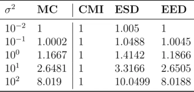
To obtain a benchmark, we compute a Monte Carlo (MC) estimate of η by performing 108 _{draws of}_X

i from N(2, σ2n), taking the Euclidean distance to Xj for each of these draws and then averaging over the computed distances. This is done to obtain an accurate approximation of the expected value the kernel. Based on that, a method is as good as its estimates are similar to the ones obtained via Monte Carlo. Table 7 shows the averaged Euclidean distance computed by each method for different values of σ2

n. Table 7 – Euclidean distance estimates.

σ2 _MC _{CMI ESD} _EED

10−2 ₁ ₁ _1.005 ₁ 10−1 _1.0002 ₁ _1.0488 _1.0045 100 _1.1667 ₁ _1.4142 _1.1866 101 _2.6481 ₁ _3.3166 _2.6505 102 _8.019 ₁ _{10.0499 8.0188}

As in Subsection 3.2.1, note that CMI computes the same approximation regardless of the value of σ2

n. This is expected, since the expected value of Xi depends only on µ. On the other hand, as shown in (EIROLAet al., 2013), the variance of the estimates is taken into account in ESD, providing more accurate results than those obtained with CMI.

While results show ESD clearly outperforms CMI, the quality of its approxima-tion degrades as σ2

n increases. In contrast to that, EED maintains a steady performance and obtains the best results for all values of σ2_{. Note also that the results presented follow} the behaviour described in Eqs. (4.9) and (4.10).

(38)

37

Thirty similar rounds of experiment were carried. In each of these, the per-centage of instances with missing samples was iteratively increased from 10% to 50% (in steps of 20%) of the dataset size. The number of features to be deleted in each of these vectors is decided independently by drawing a number from {1,· · · ,⌈D/3⌉}. In each step we use different methods to estimate the pairwise distance matrix and measuring the RMSE between these estimates and the true distance matrix computed beforehand. In this experiments, the true distribution of the data is unknown, thus, at each step we estimate a GMM, as specified by Mesquita et al. (2017) .

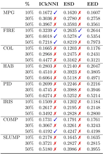
As in subsection 3.2.2, we do not consider CMI in this experiment, as it was consistently outperformed by the other methods in the previous experiment. Instead, we substitute it by the ICkNNI, using the parameters suggested in Hulse e Khoshgoftaar (2014). Results, in terms of average RMSE, are presented in Table 8. We employed Wilcoxon’s signed-rank test, with a 5% significance level, to verify the statistical significance of the results. The symbols ✓_and ✗ _{indicate the result of the hypothesis test (}✓ _{fail to reject,}

(39)

Table 8 – Euclidean distance estimation on real-world data: average RMSE

% ICkNNI ESD EED

MPG 10% 0.1672 ✓ 0.1620 ✗ 0.1607 30% 0.3036 ✗ 0.2780 ✗ 0.2758 50% 0.3967 ✗ _0.3593 ✗ _0.3561

FIRE 10% 0.3239 ✓ 0.2635 ✓ 0.2644 30% 0.6018 ✓ 0.5278 ✓ 0.5354 50% 0.7218 ✓ 0.8219 ✗ 0.7973 COL 10% 0.1665 ✗ 0.1203 ✗ 0.1176 30% 0.2968 ✗ 0.2475 ✗ 0.2431 50% 0.4477 ✗ _0.3162 ✗ _0.3121

HAB 10% 0.2803 ✗ _0.2140 ✗ _0.2047

30% 0.4510 ✗ 0.3923 ✗ 0.3805 50% 0.6064 ✗ 0.5118 ✗ 0.4971 PID 10% 0.2699 ✗ 0.2246 ✗ 0.2216 30% 0.4745 ✗ _0.3988 ✗ _0.3946

50% 0.6274 ✗ 0.5252 ✗ 0.5214 IRIS 10% 0.1509✗ _0.1202 ✗ _0.1184

30% 0.2617 ✗ 0.2195 ✗ 0.2148 50% 0.3492 ✗ 0.2828 ✗ 0.2800 COMP 10% 0.1731 ✓ 0.1791 ✗ 0.1761 30% 0.3067 ✗ _0.3261 ✗ _0.3243

(40)

39

With regard to the RMSE performance, we observe that EED outperforms CMI and ESD in all scenarios, i.e., with small and large amount of missing data. As expected, the performance gap between EED and ESD is smaller than the gap between EED and CMI. The hypothesis test indicates significant difference between EED and the other methods.

4.3 Conclusion

In this chapter, we presented a methodology to estimate the Euclidean distance between two feature vectors Xi and Xj when one or both count on missing entries. The proposed method computes the expected value of the squared-root transform z1/2 _{of the} random variable z =_kXi−Xjk2. As in the previous chapter, we assumez can be modelled with a Gamma distribution. As a consequence, z1/2 _{is Nakagami-distributed and its} expected value can be easily obtained from the distribution parameters.

(41)

5 EPANECHNIKOV KERNEL

Given twoD-dimensional vectorsXi = (xi,1, . . . , xi,D)T andXj = (xj,1, . . . , xj,D)T, the Epanechnikov kernel is given by:

k(Xi, Xj),

1₋ kXi−Xjk 2 l

p

=l−p(l₋z)p, (5.1)

wherep∈N_{− {}₀_} _and _l_∈R+ _{are kernel hyper-parameters.}

In this Chapter, we present a methodology to estimate k(Xi, Xj) when vectors

Xi, Xj ∈ X count on one or more missing components. As in the previous Chapters, it is assumed z _∼Gamma(α, β).

5.1 Formulation

Note that the Epanechnikov kernel k(Xi, Xj) is ap-th order polynomial of z and can be expanded to yield:

k(Xi, Xj) = p X r=0 p r

(l)−r(₋z)r, (5.2)

consequently, due to the linearity of expectation, estimating k(Xi, Xj) resumes to compu-ting:

E_[_k₍_X_i_{, X}_{j)] =} p X r=0 p r

(₋l)−rE_[_zr_]_, _(5.3)

which is a weighted sum of the non-central moments ofz. As in the previous chapters, we assume z ∼Gamma(α, β) . Therefore, its i-th non-central moment E_[_zi_{] is given by:}

E_[_zi_{] =}_β−iΓ(α+i)

Γ(α) , (5.4)

and, since i is a non-negative integer, eq. (5.4) simplifies to:

E_[_zi_{] =}_β−i i−1 Y j=0

(α+i). (5.5)

(42)

41

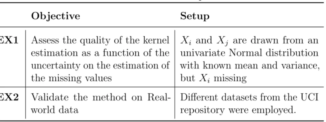
We perform two different experiments to validate our methodology (EEK) . In the first, we study how the uncertainty on the estimation of the missing values affects the quality of the kernel estimate. In second, we evaluate EEK on real-world data. Table 9 summarizes the details of these experiments. The following subsections present and discuss the results.

Objective Setup

EX1 Assess the quality of the kernel estimation as a function of the uncertainty on the estimation of the missing values

Xi and Xj are drawn from an univariate Normal distribution with known mean and variance, but Xi missing

EX2 Validate the method on Real-world data

In the first experiment, EEK is compared against the CMI, and ESD. As in the case of methodologies proposed in previous chapters, EEK differs from these methods fundamentally in the level in which the estimation problem is cast. The conceptual differences between CMI, ESD and EEK are explicitly shown in Eqs. (4.6) to (4.8).

ˆ

kEEK(Xi, Xj) = E " _p X r=0 p r

(−l)−rkXi−Xjk2r #

, (5.6)

ˆ

kESD(Xi, Xj) = p X r=0 p r

(₋l)−rE_k_X_i₋_X_j_k2r_, _(5.7)

ˆ

kCM I(Xi, Xj) = p X r=0 p r

(−l)−rkE_[_X_i]₋E_[_X_j_]_k2r_. _(5.8)

For the case in which Xi andXj abide to the conditions that makez a Gamma-distributed random variable, when pis such that g(ν) =νp _{is convex, applying Jensen’s} inequality directly to Eq. (5.6) we obtain:

ˆ

(43)

For this experiment, we set the kernel hyperparameters p = 2 and l = 40. Furthermore, we fix Xj = 3 and assume Xi ∼ N(2, σn2). Since the distribution of Xi is known, there is no need to estimate a model for the data as the true distribution _N(2, σ2

n) is given.

To obtain a benchmark, we compute a Monte Carlo (MC) estimate of the kernel by performing 108 _{draws of}_X

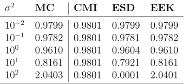
i fromN(2, σn2), taking the Euclidean distance toXj for each of these draws and then averaging over the computed distances. This is done to obtain an accurate approximation of the expected value of the kernel. Based on that, a method is as good as its estimates are similar to the ones obtained via Monte Carlo. Table 10 shows the average Epanechnikov kernel computed by each method for different values of σ2

n. Table 10 – Epanechnikov kernel estimates.

σ2 _MC _CMI _ESD _EEK

10−2 _0.9799 _{0.9801 0.9799 0.9799} 10−1 _0.9782 _{0.9801 0.9781 0.9782} 100 _0.9610 _{0.9801 0.9604 0.9610} 101 _0.8161 _{0.9801 0.7921 0.8161} 102 _2.0403 _{0.9801 0.0001 2.0401}

Observe that CMI computes the same approximation regardless of the value of

σ2

n. This is expected, since the the expected value ofXi depends only on µ. While both CMI and ESD quickly deteriorate as σ2

n increases, EEK is consistent, approximating the MC estimate more accurately. Note that results above presented respect Eq. (5.9).

We evaluate the performance of EEK on real-world datasets. For that purpose, five datasets were selected from the UCI Machine Learning Repository (LICHMAN, 2013). Further details on these datasets are available in Table 11.

Table 11 – Data sets description

Dataset Size Features

IRIS 150 4

HAYES 160 3

HABERMAN (HAB) 306 3

(44)

43

Thirty similar rounds of experiment were carried out. In each of these, the percentage of instances with missing samples was iteratively increased from 10% to 50% (in steps of 20%) of the dataset size. The number of features to be deleted in each of these vectors is decided independently by drawing a number from {1,· · · ,⌈D/3⌉}. In each step we use different methods to estimate the kernel matrix and measuring the RMSE between these estimates and the true kernel matrix computed beforehand. The process was repeated for eachp_{∈ {}2,3,4_}. In this experiments, the true distribution of the data is unknown, thus, at each step we estimate a GMM comprising three components.

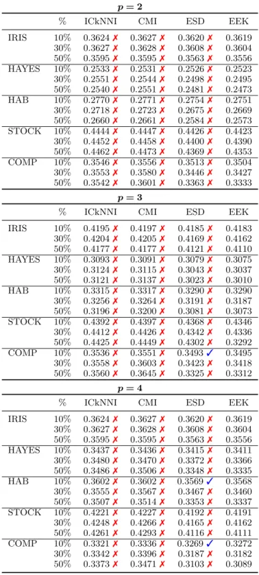
As in Subsection 3.2.2, we do not consider CMI in this experiment, as it was consistently outperformed by the other methods in the previous experiment. Instead, we substitute it by the ICkNNI, using the parameters suggested in Hulse e Khoshgoftaar (2014). Results, in terms of average RMSE, are presented in Table 12. We employed Wilcoxon’s signed-rank test, with a 5% significance level, to verify the statistical significance of the results. The symbols ✓_and ✗ _{indicate the result of the hypothesis test (}✓_{fail to}

reject, and ✗ _reject).

With regard to the RMSE performance, we observe that EEK outperforms CMI and ESD in most scenarios, i.e., with small and large amounts of missing data. As expected, the performance gap between EEK and ESD is smaller than the gap between EEK and CMI. The hypothesis test indicates, in most cases, significant difference between EEK and the other methods.

5.3 Conclusion

In this Chapter, we presented a methodology to estimate the Epanechnikov kernel between two feature vectors Xi and Xj when one or both count on missing entries. The proposed method computes the expected value of the kernel as a transform of the random variable z = kXi −Xjk2. As in the previous chapters, we assume z can be modelled with a Gamma distribution. As a consequence, E_[_k₍_X_i_{, X}_j_{)] becomes a weighted} sum of first pnon-central moments of z and can be easily obtained from the distribution parameters.

(45)

Table 12 – Comparison between EEK and other methods.

p= 2

% ICkNNI CMI ESD EEK

IRIS 10% 0.3624✗ 0.3627✗ 0.3620✗ 0.3619 30% 0.3627✗ _0.3628✗ _0.3608✗ _0.3604

50% 0.3595✗ _0.3595✗ _0.3563✗ _0.3556

HAYES 10% 0.2533✗ 0.2531✗ 0.2526✗ 0.2523 30% 0.2551✗ 0.2544✗ 0.2498✗ 0.2495 50% 0.2540✗ 0.2551✗ 0.2481✗ 0.2473 HAB 10% 0.2770✗ _0.2771✗ _0.2754✗ _0.2751

30% 0.2718✗ _0.2723✗ _0.2675✗ _0.2669

50% 0.2660✗ _0.2661✗ _0.2584✗ _0.2573

STOCK 10% 0.4444✗ 0.4447✗ 0.4426✗ 0.4423 30% 0.4452✗ 0.4458✗ 0.4400✗ 0.4390 50% 0.4462✗ 0.4473✗ 0.4369✗ 0.4353 COMP 10% 0.3546✗ _0.3556✗ _0.3513✗ _0.3504

30% 0.3553✗ _0.3580✗ _0.3446✗ _0.3427

50% 0.3542✗ _0.3601✗ _0.3363✗ _0.3333

p= 3

IRIS 10% 0.4195✗ 0.4197✗ 0.4185✗ 0.4183 30% 0.4204✗ 0.4205✗ 0.4169✗ 0.4162 50% 0.4177✗ 0.4177✗ 0.4121✗ 0.4110 HAYES 10% 0.3093✗ _0.3091✗ _0.3079✗ _0.3075

30% 0.3124✗ _0.3115✗ _0.3043✗ _0.3037

50% 0.3121✗ _0.3137✗ _0.3023✗ _0.3010

HAB 10% 0.3315✗ 0.3317✗ 0.3290✗ 0.3290 30% 0.3256✗ 0.3264✗ 0.3191✗ 0.3187 50% 0.3196✗ 0.3200✗ 0.3081✗ 0.3073 STOCK 10% 0.4392✗ _0.4397✗ _0.4368✗ _0.4346

30% 0.4412✗ 0.4426✗ 0.4342✗ 0.4336 50% 0.4425✗ 0.4449✗ 0.4302✗ 0.3292 COMP 10% 0.3536✗ 0.3551✗ 0.3493✓ 0.3495 30% 0.3558✗ _0.3603✗ _0.3423✗ _0.3418

50% 0.3560✗ _0.3645✗ _0.3325✗ _0.3312

p= 4

IRIS 10% 0.3624✗ 0.3627✗ 0.3620✗ 0.3619 30% 0.3627✗ 0.3628✗ 0.3608✗ 0.3604 50% 0.3595✗ 0.3595✗ 0.3563✗ 0.3556 HAYES 10% 0.3437✗ 0.3436✗ 0.3415✗ 0.3411 30% 0.3480✗ _0.3470✗ _0.3372✗ _0.3366

50% 0.3486✗ _0.3506✗ _0.3348✗ _0.3335

HAB 10% 0.3602✗ 0.3602✗ 0.3569✓ 0.3568 30% 0.3555✗ 0.3567✗ 0.3467✗ 0.3460 50% 0.3507✗ 0.3514✗ 0.3353✗ 0.3337 STOCK 10% 0.4221✗ _0.4227✗ _0.4192✗ _0.4191

30% 0.4248✗ _0.4266✗ _0.4165✗ _0.4162

50% 0.4261✗ _0.4293✗ _0.4116✗ _0.4111

(46)

45

6 EXPECTED VALUE OF BASIS FUNCTIONS

Single-Layer Feedforward Neural Networks (SLFNNs) can often be expressed in terms of basis expansion functions, i.e., the predicted output ˆy ∈R _{for an input vector}

X _∈RD _{can be expressed as}

ˆ

y = H X h=1

κhφh(X). (6.1)

whereφh :RD →Ris the activation function of the h-th hidden neuron and κh ∈R is the weight of the link between this neuron and the output node.

For instance, for conventional Random Neural Networks (RNNs) using the sigmoid (also known as logistic) activation function, we have:

ˆ

y = H X h=1

κhg(λh·X) (6.2)

where g(t) = 1/(1 +e−t_{) and} _λ

h ∈RD is the vector of weights that links the input layer to the h-th hidden neuron. Thus, φh can be written as a non-linear transform of λh·X. This is also true - with different expressions for g(_·) - for Single-Layer Feedforward Neural Network (SLFNN)s using the hyperbolic tangent, logit, probit or cosine as the activation function.

On the other-hand, for centroid-based SLFNNs , such as Radial Basis Function Networks and q-Generalized Random Neural Networks, Eq. (6.1) is equivalent to:

ˆ

y = H X h=1

κhg(kX−λhk2) (6.3)

with λ∈RD _{now as the} _h_{-th centroid of the network.}

(47)

6.1 Formulation

The problem of estimating φ(X) for a D-dimensional vector X counting on missing entries consists in computing

E_[_φ₍_X_{)] =} Z

RD

φ(X)p(X)dX, (6.4)

for which there is no trivial general solution and tailored ones depend on both the format of φ(_·) and p(_·). However, for any φ(_·) and p(_·), it is possible to approximate Eq. (6.4) via sampling or numerical integration methods.

The UT, originally proposed in (JULIER; UHLMANN, 1997), is a sampling-based method for estimating statistical moments of a probability distribution associated to a random variable which results from a nonlinear transformation of another random variable (LE ˜AO; YONEYAMA, 2011).

In order to estimate φ(X) using the UT, a set_S = _{γl}Ll=1 ⊂RD of sigma points (SPs), with respective weights {kl}L

l=1 ⊂ R, associated to the original random variable X are deterministically chosen. Then, the SPs are passed through φ(_·), resulting in a transformed set of SPs. Finally, the transformed SPs (and their corresponding weights) are used in order to approximate E_[_φ₍_X_{)]. Although there is no restriction on their sign,} the weights k1,· · · , kL must respect the convexity constraint

L X

l=1

kl = 1 (6.5)

to provide an unbiased estimate (JULIER; UHLMANN, 2004).

The implementation of the UT to estimate φ(X) can then be summarized by the following equations:

δl ←φ(γl) ∀1≤l≤L, (6.6)

E_[_φ₍_X_)]_≈ L X

l=1

klδl. (6.7)

There are different possible ways to choose the SPs and respective weights. Let

(48)

47

Equations (6.8) to (6.11).

γ1=E[X] (6.8)

γl=γ1+ hp

|M_|Σi

l−1 ∀1< l≤ |M|+ 1 (6.9)

γl=γ1− hp

|M|Σi

l−(d+1) ∀d+ 1 < l≤2|M|+ 1 (6.10) kl=

1

2|M|+ 1 ∀1≤l≤2|M|+ 1 (6.11) wherehp

|M_|Σi

l denotes the l-th row of the matrix square root of |M|Σ, which is the covariance matrix Σ of XM (conditioned on XO) multiplied by the number of missing entries _|M_|.

Although this UT approach could be applied directly to estimate the value of arbitrary basis expansion functions in our context, the number of required samples L

grows with the number of missing entries, which could make it computationally inefficient when X counts on many missing features.

To alleviate this problem, we propose two methodologies based on the UT that require only three one-dimensional sigma points, independent of _|M_|. The first one, presented in Subsection 6.1.1, is tailored to the sigmoid function and can be easily generalized to any φ(_·) that can expressed as transform of λ_·X. The latter, in Subsection 6.1.2, deals with theq-Gaussian function and can be adapted for anyφ(·) that is a transform of _kX₋λ_k2_.

6.1.1 Sigmoid Function

Given an input vector X = (x1, . . . , xD)T, the sigmoid function is given by:

fσ(X) = 1

1 +e−λ·X, (6.12)

in which λ= (λ1, . . . , λD)T is a predefined constant vector.

Note that fσ(X) can be written as a transform of the random variable λ_·X, whose expectation is given by:

E_[_λ_·_X_{] =} D X d=1

λdE[xd], (6.13)

and has variance:

Var[λ_·X] = D X

d=1

(49)

Using the aforementioned UT scheme, we can approximate E_[_f_σ(_X_{)] using} _L_{= 3 sigma} points as follows:

E_[_f_σ(_X_)]_≈ X i∈{−1,0,1}

1 + exp{−E_[_λ_·_X_]₋_i_Var[_λ_·_X_]_}−1

3 (6.15)

It is important to notice this methodology also applies to any transform of X

that can be written as a function of λ·X.

6.1.2 q-Gaussian Function

For an input vector X = (x1, . . . , xD)T, the q-Gaussian activation function can be expressed as:

G(X) =eq(−kX−λk2_ν−1₎ _(6.16)

whereλ = (λ1, . . . , λD)T, ν >0 and q ∈Rare predefined constants while

eq(t) = [1 + (1−q)t]

1

1₋t. (6.17)

Note thatG(X) can be written as a transform of kX−λk2_{, whose expectation is given by}

E_[_k_X₋_λ_k2_{] =} D X d=1

(E_[_x_d]₋_λ_d)2_{+ Var[}_x_d]_, _(6.18)

and has variance:

Var[_kX₋λ_k2] = D X

d=1 E_[_x4

d]−E[x2d]2+ 4λ2dVar[xd]. (6.19)

Thus, E_[_G₍_X_{)] can be approximated using the aforementioned UT scheme with exactly}

L= 3 sigma points, as follows:

E_[_G₍_X_)]_≈ X i∈{−1,0,1}

eq(−(E_[_k_X₋_λ_k2_{] +}_ip_Var[_k_X₋_λ_k2_])_ν−1₎

3 (6.20)

Notice that this methodology can be trivially adapted to estimate the value of any specific transform φ(X) that can be expressed as a function of _kX₋λ_k2_.