Abstract
To study the influence of a foundation structure on the ground, the finite layer method of composite ground is derived based on the finite layer method (FLM) theory of the semi-analytic numeri-cal method and the force method principle of elastic material, which is used to analyze a layered ground including multiple in-ternal constraint planes. By simplifying a pile body as a solid constraint composed of four side plane constraints, the composite ground FLM is applied to solve the displacement and stress field of the ground. The change of the ground displacement and stress caused by the addition of a single pile constraint are then dis-cussed, and the influence rules of a pile position on the ground displacement are also determined. Finally, the necessity, rationali-ty and validirationali-ty of the composite ground FLM are demonstrated by the model test examples of a single pile and pile raft foundation.
Keywords
Composite ground FLM; Force method principle; Internal con-straint plane; Pile foundation.
The Composite Ground Finite Layer Method
and its Application to Pile Foundation Analysis
1 INTRODUCTION
The multilayer property is a common characteristic of natural ground, and the analysis of layered ground is an important subject in geotechnical engineering. In ground and foundation engineering problems, foundation structures have been added to the original ground so that the interaction be-tween the ground and structural members under the upper load changes the mechanical state of the ground. For example, the shielding and reinforcement effects of a pile group are objective. Neglect-ing the influence of the pile body on the ground properties may lead to an excessively large settle-ment calculation. Therefore, for layered ground with structure members (such as a pile group),
Guan Feng Tian a Lian Sheng Tang b Hong Wei Ma a Qi Xing Wu a
a Key Lab of Disaster Forecast &
Con-trol Engineering, Jinan University, Guangzhou 510632, PR China
b School of Earth Science and Geological
Engineering, Sun Yat-sen University, Guangzhou 510275, PR China (Corre-sponding author)
E-mail: [email protected].
http://dx.doi.org/10.1590/1679-78252668
which is called “composite ground”, the method by which its mechanics are analyzed is an important prerequisite for the study of the interaction between the soil and structure.
At present, the following research methods of ground and foundation interaction are used: finite element method (Comodromos et al., 2009), boundary element method (Ai and Han, 2009), infinite layer method based on the superposition principle (Cheung et al. 1988), calculation model simplified method (Cairo & Conte, 2006 and Zhang et al., 2010), elastic analytical method based on the ener-gy principle (Seo & Prezzi, 2007), data analysis methods based on an artificial neural network (Is-mail & Jeng, 2011) and support vector machine (Farfani et al., 2015). The mixed method of the boundary element method and finite element method has been commonly used in theoretical studies by Millán and Domínguez (2009), Vasilev et al.(2015). Another mixed method of the analytical layer element method and boundary element method is occasionally used by Ai and Cheng (2013). Based on the characteristics and advantages of each method, the development of the number meth-od, analytical method and intelligent analysis method embodies the diversity of research ideas.
The application of the above mixed methods is more flexible and can more effectively achieve the advantages of single methods. With regard to the research subject, most of the literature focuses on the deformation and bearing characteristics of the foundation under the condition of ground and foundation interactions. However, the change in the mechanical properties of the ground caused by adding foundation structural members has attracted little attention for further study. Thus, if the mechanical analysis of ground space is considered as the research basis and the exertion of structur-al members as an additionstructur-al condition, the change of ground properties can be sequentistructur-ally solved when the structural member changes to lead to mutual influence between the ground and founda-tion structure.
According to the present literature, the solution of layered ground mainly includes the
numeri-cal analysis method by Krasiński (2014) and Mendoza et al.(2015), analytic method by Ai et
al.(2012), and semi-analytical numerical method. With the rapid development of computer technol-ogy and the wide application of ABAQUS, ANSYS, FLAC3D, MIDAS and other large finite ele-ment software applications, the finite eleele-ment method has notable advantages in solving the ground characteristics of three-dimensional space, which is convenient and adaptable. However, in the anal-ysis of layered soil and foundation interaction, the large sizes of the elements and the solving equa-tion may greatly increase the computaequa-tion time because of the difficulty in improving the accuracy of the calculation. The representative analytical method is the analytical layer element method for solving multilayered soils proposed by Ai et al. (2014). Based on the basic control equation of the three-dimensional problem of elasticity mechanics, the solution to the analytical layer element of the layered ground problem in the physical domain can be obtained by Fourier transform and decou-pling transformation technology according to the principle of the finite layer method (FLM). This method has been applied to the consolidation problem and dynamic response of layered ground. The advantages of the analytical method lie in that the theoretical principle is clear and the calculation efficiency and accuracy are relatively high. However, its limitation is reflected in the difficulty in the improvement of the theoretical solution in handling more complex ground, including heterogeneous layer elements.
basis for further research. In early research, the FLM was proposed by Cheung et al. (1982) for the analysis of structural components as a semi-analytic numerical method. Booker and Small et al. (1982a, 1982b, 1987) then developed the FLM to adapt to the layered ground and applied it to consolidation problem and shallow foundation analysis by Swaddiwudhipong et al.(1992) and Sen-juntichai et al.(2006).
In this paper, the FLM is used as the primary theory, layered ground is used as the main sub-ject, and piles or other structural members are used as internal constraints. With the aim of compo-site ground analysis, the following development is continued: First, based on the FLM principle, the solving process of the ground with internal constraint planes will be deduced to technically consti-tute the composite ground FLM by applying the force method of elastic mechanics. Second, by sim-plifying the pile body constraint, the composite ground FLM will be used to analyze the influence of a single pile constraint on ground displacement and stress. Finally, the composite ground FLM re-sults of a single pile and pile raft foundation will be used to compare with the model test rere-sults to verify the rationality of the former.
2 FINITE LAYER METHOD OF COMPOSITE GROUND
2.1 Finite Layer Method of Ground with Homogeneous Layers
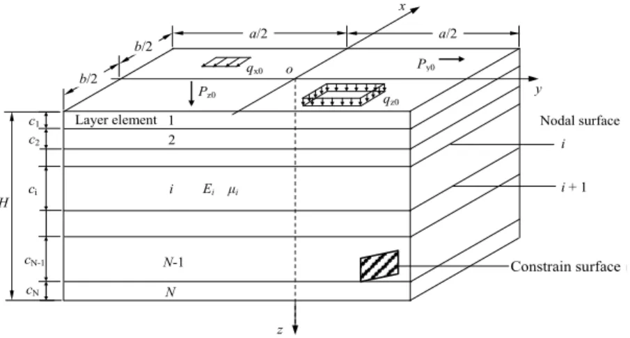
The ground with homogeneous layers is assumed to be a semi-infinite elastic space and is simulated by a finite body model that is sufficiently large with a plane size a×b and thickness H, as shown in Figure 1. This body consists of N layer elements. For element i with thickness ci including the
up-per and lower nodal surfaces i and i+1, the material parameters include the elastic modulus Ei (In
theoretical analysis E is often replaced by deformation modulus E0 for layers) and Poisson’s ratio μi .
The bottom support condition of the body model is assumed to be rigid and rough, and the four side boundary conditions are supported simply.
Figure 1: Analysis model schematic of ground with homogeneous layers.
Any directional load can be formed by the superposition of four types of different symmetrical forms. For example, based on the basic principles of the FLM, the displacement functions of each
a/2 a/2
b/2 b/2
y x
z o
H c1
c2
ci
cN-1
cN
Pz0
Py0
qx0
qz0 Layer element 1
2
i
N N-1
Ei μi
Nodal surface
i
i + 1
layer element under the biaxial symmetrical vertical load with the x and y axes can be described as follows:
x
(1)
where u, v, and w are the displacements of a layer element in the y and z directions, respectively; km=mπ/a; kn=nπ/b; and m and n are series numbers with maximum values r and s, respectively.
The polynomial functions f (z), f (z), fw(z)
mn v
mn u
mn are used to indicate changes along the z-direction of
the three-dimensional displacements:
x
(2)
in which a1i,mn, a2i,mn, a3i,mn, i=1,2,…,6, are the polynomial coefficients of three-dimensional
dis-placement functions. The coefficient vectors are assumed T
mn j mn j mn j mn j mn j mn j mn
j a a a a a a
a} { , , , , , }
{ 1, 2, 3, 4, 5, 6, ,
j=1,2,3. The quintic full polynomial is selected for the functions in Eq. (2) based on the fact that the number of degrees of freedom of a layer element is six, corresponding to six displacements in three directions of the upper and lower nodal surfaces.
According to the condition of the static equilibrium equation at any point in the elastic layer, it is deduced that due to the correlation among the 18 coefficients discovered by the elastic formulae transformation, the number of independent coefficients is 6, which is the number of nodal surface displacements of the layer element. For a layer element, assuming that the displacement vector of its upper and lower nodal surfaces is
{δ}mn={umni ,vmni ,wimn,umnj ,vmnj ,wmnj }T (3)
The displacement vector of an arbitrary point of the layer element is
∑ ∑
1 1 } { ] [ } , , { } { r m s n mn mn T N w v u f (4)
in which the shape function matrix is
∑
6 1 1 -, 1 ) ( i i mn i umn z a z
f
∑
6 1 1 -, 2 ) ( i i mn i vmn z a z
f
∑
6 1 1 -, 3 ) ( i i mn i wmn z a z
f
∑ ∑
1 1 sin cos ) ( r m s n n m vmn z k x k y
f v
r m s n n m umn z k x k y
f u 1 1 cos sin ) (
∑ ∑
1 1 cos cos ) ( r m s n n m wmn z k x k y
f w
{N} mn = 36 35 34 33 32 31 26 25 24 23 22 21 16 15 14 13 12 11 N N N N N N N N N N N N N N N N N N (5)
According to the definition of the layer element strain vector, the strain matrix [B]mn can be
deduced. The stiffness matrix of the layer elements can then be written as [S]mnmn=
V mnT
mn D B dV
B
[ ] [ ][ ] , which can be calculated using the 5-point Gaussian integral method. Assuming
a distributed body load vector {q}={qx, qy, qz}T, the equivalent load vector of the layer element can
be obtained by the following formula:
T mn w j v j u j w i v i u i e
mn
F
F
F
F
F
F
F
}
{
,
,
,
,
,
}
{
=
V T mn q dV N] { }
[ (6)
For the multilayer ground model of N layer elements, all layer element stiffness matrices [S]mnmn
and load vectors e
mn F}
{ are assembled to form the global stiffness matrix [K]mn and load vector
{F}mnof order 3N+3. After modifying matrix [K]mn according to the ground conditions, the system
static equilibrium equation can be solved to obtain the displacement parameter vectors {δ}mn of the
nodal surfaces. Additionally, the displacement, stress, and strain of an arbitrary ground point can be obtained. Finally, after performing series calculation cycles r×s times, the final resolution can be obtained. To simplify, the homogeneous-layered ground FLM is abbreviated “HLG-FLM” in the following text.
2.2 Finite Layer Method of Ground with an Internal Plane Constraint 2.2.1 Single Internal Plane Constraint Analysis
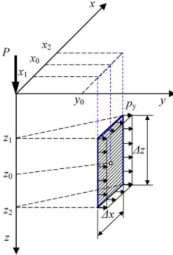
Figure 2 shows the coordinate system of a semi-infinite space model of ground with an external load P at the origin. A vertical plane constraint S exists with center coordinates (x0,y0,z0), height Δz and
width Δx .
The displacement condition of constraint plane S means that the horizontal displacement is in the y direction, v=0, in the domain with x∈[x1,x2],z∈[z1,z2], and y =y0, in which x1=x0 –Δx/2,
x2=x0+Δx/2, z1=z0 –Δz/2, z2=z0+Δz/2. It is assumed that the constraint reaction of constraint
plane S is uniformly distributed with its direction consistent with the y axis when the area of plane S is relatively small. According to the principle of the force method for statically indeterminate structure analysis, the calculation steps of constraint plane S are as follows.
When the original load is acting on unconstrained ground, HLG-FLM can be used to obtain the horizontal displacement v0 of plane S. The average displacement
v
of S is estimated by the loading unit constraint distributed forcep
y=1 kPa in the ground without external any load. Based on the constraint plane condition, which means that v=0 for the arbitrary point of S, the horizontal dis-placement equation isv0 + py
v
=0 (7)Then, py=v0/
v
, which is the real constraint force of plane S. In Figure 2, a vertical constraintplane parallel to the x axis is defined as a “V” type because of its displacement characteristic v=0. Similarly, a “U”-type vertical constraint plane means that its displacement u=0.
2.2.2 Multiple Internal Plane Constraint Analysis
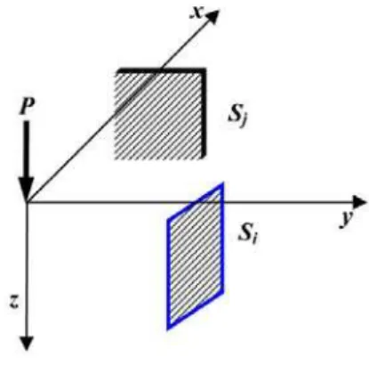
There are multiple vertical plane constraints in ground with original load P, Si, i=1, 2, ···, ms, as
shown in Figure 3, which constrain horizon displacements i , i=1, 2, ···, ms, respectively.
Figure 3: Multiple vertical plane constraints in ground.
When multiple plane constraints exist in the ground, the principle of mechanical superposition is used to analyze it as follows:
By applying unit constraint force
p
i=1 kPa at the position of single constraint plane Si, thehorizontal displacement
ji of all constraint planes Sj, including itself when i=j, can be calculated.With consideration of stress superposition of all constraint forces, the displacement condition of constraint plane Sj is
0
01
jms
i ji i
p
, j=1, 2, ···, ms (8)where pi is the constraint force distributed value of plane Si. After solving the above ms equations
using Eq.(8), the solution of constraint force pi(i=1, 2, ···, ms) can be obtained.
2.2.3 Finite Layer Method of Ground with Multiple Constraints
When there are ms plane constraints in the ground, the following steps are suggested for ground analysis:
First, the original loading state of the ground model should be determined according to the ac-tual external loads. The types and displacement conditions of the added plane constraints in the ground must then be determined.
Second, constraint force pi (i=1, 2, ···, ms) can be obtained by the multiple internal plane
con-straint analysis process in 2.2.2. In Figure 2 and Figure 3, the four corner coordinates of U-type constraint plane Sj are [xj, yj – Δyj/2, zj – Δzj/2], [xj, yj +Δyj/2, zj – Δzj/2], [xj, yj +Δyj/2, zj +Δzj/2]
and [xj, yj – Δyj/2, zj +Δzj/2]; constraint force vector pj can then be formulated as
{p}j={px, py, pz}Tj=pj {1, 0, 0}T=pj ex (9)
where ex ={1, 0, 0}T is the unit vector along the x axis.
Third, the constraint force vector can be transferred into the equivalent nodal surface load vec-tor of the layer element with constraint plane Sj, which is
j S x j T mn
e N p e dS
P
j
j
[ ]}
{ (10)
The shape function matrix of Eq. (5) is substituted into Eq. (10); then,
j S mn j e dS N N N N N N N N N N N N N N N N N N p P j j 0 0 1 } { 36 26 16 35 25 15 34 24 14 33 23 13 32 22 12 31 21 11
T mnP
P
P
P
P
P
,
,
,
,
,
}
{
1 2 3 4 5 6
(11)where
j
s
j k j
k p N dS
P 1 , k=1, 2, ···, 6.
{p}i ={px, py, pz}Ti=pi {0, 1, 0}T=pi ey (12)
where ey={0, 1, 0}T is a unit vector along the y axis.
The equivalent nodal surface load vector of the layer element with constraint plane Sj is as
fol-lows:
i S
y i T mn e
i N pe dS
P
i
[ ]
}
{
iS
T mn
i N N N N N N dS
p
i
26 25 24 23 22 21
(13)
HLG-FLM is carried out to obtain constraint force pi using Eq. (8).
Finally, the ground is assumed to be under the original load and all of the constraint forces, which can be solved by HLG-FLM.
2.3 Composite Ground FLM
If the composite ground contains solid structure constraints that can be decomposed into multiple constraint surfaces, the above FLM of ground with multiple constraints will be used for ground analysis. All above contents of this section are concluded with regard to the semi-analytical numeri-cal method of the FLM for composite ground.
3 COMPOSITE GROUND FLM APPLICATION IN PILE FOUNDATION
3.1 Simplification of Pile Constraint 3.1.1 Single Pile Constraint
In pile foundation analysis, the constraints in layered ground are vertical piles. It is assumed that a pile constraint is an elastic member with consideration of the vertical compression deformation of itself. The vertical displacement of the pile body and that of the lateral soil are coordinated with each other.
Generally, the rigidity of a pile is considerably higher than the ground soil. Thus, the pile body can obstruct the horizontal displacement transfer of the soil between piles for its shielding effect, with the result that the normal displacement is zero and the tangential displacement is not zero for all constraint planes of the pile body. Therefore, based on the displacement characteristics of the pile constraint, only the constraint effect on the lateral displacement of the pile side is considered here. The analysis of displacement to the origin load P of a square cross-section pile constraint is simplified by the projection method, as shown in Figure 4. The prism of the square pile is projected onto the three axes of the coordinate system; the top and bottom surfaces are not considered tem-porarily because they cannot constrain the horizontal displacements. For four lateral surfaces of the pile, they are regarded as V type constraint plane Si, S′i, and U-type constraint plane Sj, S′j.; thus,
the pile body constraint is replaced with four vertical constraint planes.
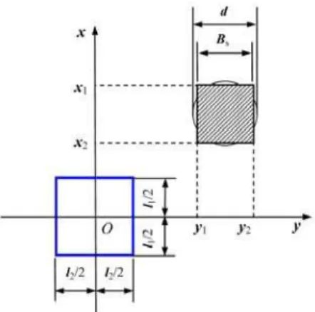
If a pile with a circular cross section exists in layered ground, the circle can be transformed into a square with the same centroid and equal area in the pile constraint analysis. As shown in Figure 5, on the ground surface, there is a distributed load with area l1×l2 and a circular cross section pile in
Eight edge-shaped cross sections have been tested to replace the circular section of the pile con-straint to calculate the ground stress and displacement at the load center. Eight vertical concon-straint planes resulted in a slow calculation speed compared with the simplified method with 4 constraint planes, but the calculation error was extremely small.
Figure 4: Projection for a square pile constraint. Figure 5: Simplification of a circular pile constraint.
3.1.2 Multiple Pile Constraints
The composite ground analysis method with multiple pile constraints is the same as that with mul-tiple plane constraints, with consideration of the cross effects of pile side constraint surfaces. In ground and pile foundation interaction analysis, the composite ground is then calculated to obtain the flexibility coefficients of the pile and soil system, which can be substituted into the upper struc-ture-pile-soil interaction equation to solve the pile foundation settlement and friction resistance of the pile side.
3.2 Influence of a Single Pile Constraint on the Stress and Displacement of Ground
The plane layout of a single pile constraint and load is shown in Figure 6. The vertical load of the ground surface q=1 kPa, and distributed area l1×l2=2.0 m×2.0 m with center point O(0,0,0) and
edge midpoint A(1,0,0).
The single pile constraint cross section Lsx×Lsy=1.0 m×1.0 m, and the pile length Hsz=20 m. It
is assumed that the pile and load are in contact with the edge and that the distance between pile constraint center and load center xs=l2/2+Lsy/2=1.5 m. The parameters of the ground are
defor-mation modulus E0=5.0 MPa and Poisson's ratio μ=0.4. The ground finite layer model size is area
a×b=50 m×50 m and depth H=30 m.
3.2.1 Influence of a Single Pile Restraint on the Vertical Displacement and Stress of the Ground Surface
Based on the composite ground FLM, the result curves along the x axis of these variables in the ground surface, including the vertical displacement w, vertical stress z, horizontal stress x and
shear stress zx, have been calculated considering the pile constraint. For comparison, HLG-FLM is
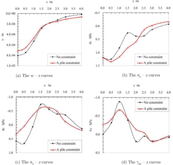
used to calculate those variables in the ground without a constraint. All results of the variables under two situations are shown in Figure 7(a)–(d).
(a) The w – x curves (b) The z – x curves
(c) The x – x curves (d) The zx – x curves
Figure 7: Displacement and stress curves of ground surface under different constraint conditions.
For the first stage, x
[0,1], the vertical displacement w of the ground surface with the pile con-straint is less than that with no concon-straint. Although loaded in this range, the lateral concon-straint effect of the pile body blocks the horizontal transmission of w.For the second stage, x
[1,2], with the pile constraint range, two curves cross a transition, which means that the constraint effect of the pile body diminishes.For the third stage, x
[2,3], after bypassing the constraint, w with the pile constraint is more than that with no constraint.See Figure 7(b), by comparing the ground surface z-x relation curve of no constraint and of a
pile constraint, it can be found that the z at x=0.0 is almost same for the two curves. However, the z maximum value of the latter is greater about 8% than the former at x=0.5 for the blocking effect
of pile constraint. When x>2.0m, z of the latter tends to be zero more quickly after bypassing
con-straint. Then from Figure 7(c), it is evident that the existence of vertical pile constrain has re-strained the transfer of x in horizontal direction so that x maximum value with a pile constraint
is smaller than that with no constraint. At last Figure 7(d) shows that the zx with pile constraint is
not zero at x=0.0, which is significantly different from that of no constraint. And after x>2.5m the effect of pile constraint on zx disappeared quickly as the coincidence degree of the two curves is
high.
Thus, despite the pile constraint being partially blocked to deduce the vertical displacement w transferred to the constraint surface from the direction of the load, w is dispersed to a farther and greater extent in the ground after bypassing the pile constraint. Figure 7(a)–(d) illustrate that the displacement and stress curves under the constraint condition change more moderately and main-tain continuity after the pile constraint on the basis of the existence of the pile body.
3.2.2 Influence of a Single Pile Restraint on the Displacements and Stresses of the Ground
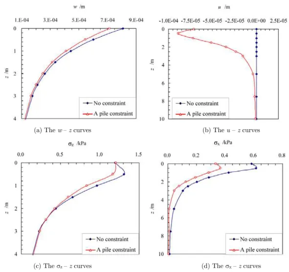
Under the two ground conditions of no constraint and a pile constraint, the result curves along the z axis of these variables at the distributed load center point O, including the vertical displacement
w, horizontal displacement u, vertical stress z and horizontal stress x, have been achieved by the
composite FLM and HLG-FLM, respectively. All results of the variables under the two situations are shown in Figure 8(a)–(d).
See Figure 8(a) at z = 0.0 m, the w of considering pile constraint is smaller 15% than that of neglecting constraint. Then the two w–z curves tend to be consistent at z=4.0 m. Similar rule hap-pens on the z –z curves in Figure 8(c) except that zero point, z=0.0, in which the z does not
change with pile constraint. However, by Figure 8(b) it is found that the u-z curve distribution form is completely changed due to the pile constraint, in which u moves to the x axis negative direction as the pile constraint is located in the positive direction. For z=0.0 to 5.0 m the u decreases sharply in general after a short increase, till z=10.0 m it almost reduces to zero gradually. From Figure 8(d),
compared with the unconstrained condition, the x at z=0.0 m declines by 43% because the pile
constraint reduces the horizontal stress transfer effect. The two x –z curves have same form,
though the x with pile constraint are smaller when z=0.0 to 10.0m.
The influence depth of a pile constraint on w and σz of point O is smaller, which is
no-constraint condition, the blocking effect of a pile body causes w, σz, and σx under point O to de-crease but u to inde-crease.
(a) The w– z curves (b) The u – z curves
(c) The z – z curves (d) The x– z curves
Figure 8: The ground displacements and stresses curves along depth z at load center O
under different constraint conditions.
3.3 Influence Rules of a Pile Constraint Position on the Displacement of Ground
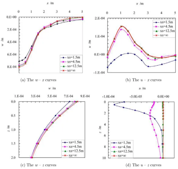
In Figure 6, in the case where other conditions are unchanged, the distance xs between the distrib-uted load center O and pile section center has been changed to solve the vertical displacement w and horizontal displacement u of load center O. The changes with different distances xs of the dis-placement curves along the x and z axes are shown in Figure 9(a)–(d).
constraint can be completely ignored. Then, it is thought that a pile constraint influence can be rationally neglected when xs>4.5 m, which means that the center distance xs between the pile and load is 3 times the load width and the constraint section (l2/2+Lsy/2=1.5 m). This result is
con-sistent with the general theory of pile foundations that the pile spacing is less than 4-6 times the pile diameter, in which there is a mutual influence between piles. The conclusion was demonstrated by Wu et al.(2004).Thus, the group of piles with pile spacing greater than 6 times the diameter of the piles is called the sparse pile foundation according to the application handbook of technical specification for building pile foundation (Liu et al., 2010).
(a) The w– x curves (b) The u – x curves
(c) The w – z curves (d) The u – z curves
Figure 9: Displacementscurves of a load center under different xs conditions.
4 EXAMPLE ANALYSIS
4.1 Single Pile Model Test
The original single pile model tests was carried by Zhang (2002), in which varied outdoor model tests of a single pile with different lengths and diameters have been carried out to study the charac-teristics of stress and strain of a single pile foundation, such as the pile top settlement and pile skin friction resistance distribution. The parameter values of the ground distribution and physical prop-erties are shown in Table 1. Because the compression modulus Es of the soil is obtained by an
in-door consolidation test, its test value is less than the real value in the field. According to geological history, test site condition and engineering experience value, the deformation modulus E0 is taken
to be 4 times Es for layers. The Poisson's ratio μ of soil is based on the empirical values of
geotech-nical engineering investigation rules. The model pile material is C30 fine concrete. The geometric dimensions, material parameters and loading conditions of the model piles are shown in Table 2.
Soil layer number
Soil classification
Layer thickness
compression modulus
Es (MPa)
deformation modulus
E0 (MPa)
Poisson's ratio μ
Silty clay 1.30–2.00 m 5.5 22 0.38
Silt 2.22–2.70 m 12 48 0.35
Fine sand 1.0–2.6 m ---- 60 0.30
Table 1: Properties of the soil in the single pile model test.
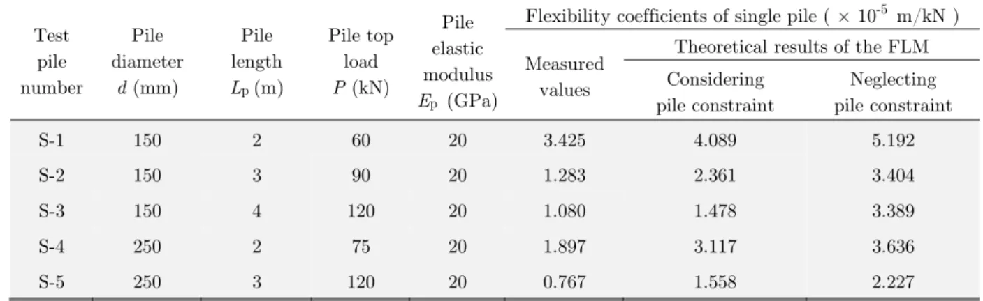
Test pile number
Pile diameter
d (mm)
Pile length
Lp (m)
Pile top load
P (kN)
Pile elastic modulus
Ep (GPa)
Flexibility coefficients of single pile ( × 10-5 m/kN )
Measured values
Theoretical results of the FLM Considering
pile constraint
Neglecting pile constraint
S-1 150 2 60 20 3.425 4.089 5.192
S-2 150 3 90 20 1.283 2.361 3.404
S-3 150 4 120 20 1.080 1.478 3.389
S-4 250 2 75 20 1.897 3.117 3.636
S-5 250 3 120 20 0.767 1.558 2.227
Table 2: Properties of the piles in the single pile model test.
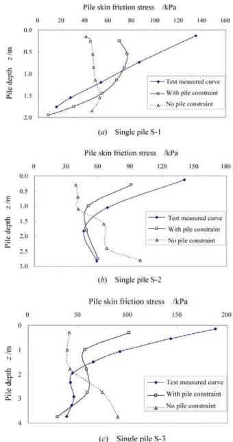
Figure 10: Pile skin friction distribution of a single pile.
For the pile flexibility coefficients in Table 2, compared with the results without considering pile constraints, the theoretical results with consideration of a single pile constraint are more con-sistent with the measured values, which shows the necessity of considering the constraint affect of the pile body in pile foundation analysis. However, soil parameters may not be highly accurate, which causes the theoretical results are still slightly larger, approximately 1.19 to 2.03 times the test values.
the vertical area stress around pile sides, which accords well with actual practice. After considering the pile constraint influences on the ground lateral displacement, the flexibility of the soil element on pile sides reduces to cause the side friction resistance of the shallow soil to improve, which is consistent with the measured results. However, in Figure 10(a), there are significant divergence between the theoretical and experimental results for pile S-1 between z=0.0 and 0.75m. The reason lies mainly in the geological fact that pile S-1 is surrounded by homogeneous silty clay with a thickness of nearly 2.0m, which means it is close to a pure friction pile. So among three piles, 1, S-2 and S-3, pile S-1 has the largest flexibility coefficient (See Table S-2) and particularly the measured skin friction stress distribution with the linear decrease of depth. Therefore, based on the greater flexibility of pile-soil system itself, the constraint effect on pile side soil is weakened relatively so that the theoretical result of pile S-1 with consideration of pile constraint deviates from the test curve at the upper 1/3 part of the pile.
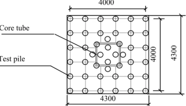
4.2 Pile Raft Foundation Model Test
The original pile raft foundation model test is studied by Liu et al. (2006), in which they studied the working characteristics of group piles in composite ground and composite pile foundation by using a field-scale model test with a model test ratio of 1:10. The pile layout under the raft is as shown in Figure 11, with a model raft thickness of 0.15 m, a model pile diameter of 150 mm and a length of 2.0 m, and the elastic modulus of the raft plate and piles is 20 GPa. The distribution of the ground layers is as follows: the first layer is silty clay with thickness 1.75 m and compression modulus Es1=5.5 MPa; the second layer is silt with a thickness of more than 2.5 m and compression
modulus Es2=12 MPa. In the original literature, to compare the different working characters of two
groups of tests, the composite ground and the composite pile foundation, the gravel sand cushion with a thickness of 100 mm was set up between the raft basement and the soil surface for the for-mer, especially under the situations with the same geological conditions and loading layouts. Con-sidering that the ground may be disturbed by test construction in the field, including site leveling and pile tip vibration, the deformation modulus of the soil is 2 times the compression modulus. The Poisson's ratio is 0.38 for silty clay and 0.35 for silt, respectively.
The average settlements of two composition foundations are solved under different loads using the composite ground FLM with the results shown in Table 3.
Figure 11: Pile layout under raft basement.
4000
4300
4000 4300 Test pile
Load of raft board P (kN)
Composite pile foundation settlement s (mm) Composite ground settlement s' (mm)
Model test Composite ground FLM
(this paper) Model test
Composite ground FLM (this paper)
1625 1.086 3.33 2.41 3.757
2438 2.361 4.85 4.25 5.499
3250 4.866 5.97 6.80 8.129
4063 7.039 7.05 10.20 9.993
Table 3: Average settlements of the pile-raft foundation.
Table 3 illustrates that the error of the theoretical results relative to the measured values is smaller for the composite ground settlement s' compared with the composite pile foundation settle-ment s. And the error decreases with increasing load P. These phenomena may be explained for two reasons. Firstly, the super-consolidation nature of soil is probably the basic reason. In the pile raft model test, the site was originally an area of about 1500m2 in dried fish pond with level bottom, which was below the natural ground 2.0m. Next to it an office building and a material processing workshop were being built. Based on the geographical condition and field situation, the shallow layers have the property of super-consolidation soil. So under small load the pile foundation has smaller settlement compared with theoretical results. However, for the foundation with larger load the super-consolidation soil effect on settlement is reduced to be tiny. Secondly, the strength differ-ence of soil-pile interaction is another reason. When the foundation settlement is greater under larg-er load, the soil between piles can play bearing capacity much bettlarg-er. Meanwhile, the pile body may play shielding effect on soil more fully. This real engineering situation can be well simulated by the composite ground FLM, with the results of very small error.
The skin friction distribution along the depth of the corner pile under the raft basement is also obtained and compared with the model test data for the composite pile foundation, which is shown in Figure 12(a)–(d). The results of the corner pile skin friction for the composite ground are shown in Figure 13(a)–(d). The pile skin friction distribution curves in Figure 12 and Figure 13 illustrate that the measured curves of the model test and the calculated curves are in good agreement with the overall trend for both the composite ground and pile foundation.
Figure 12: Pile skin friction distribution of the composite pile foundation under varied load.
The comparison and discussion of the model test results and theoretical calculation results of a single pile and a pile raft foundation demonstrate that the composition ground FLM of this paper is adaptable to the interaction analysis of a pile foundation and effective in adding constraints to lay-ered ground research. Also the example analysis shows the necessity of considering the constraint of the pile body in ground and foundation studies.
5 CONCLUSIONS
In the interaction analysis of ground soil and foundation structures, the original mechanical proper-ties of ground change based on the additional application of structural members. To explore the change rules of ground properties, the research idea of multilayer composite ground is formed by adding internal constraints to natural ground. A multilayer ground model is established based on the FLM theory of the semi-analytical numerical method. By adding single, multiple and different directions of plane constraints and even solid constraints to the ground, the composite ground FLM is deduced in detail according to the force method principle for elastic material.
The composite ground FLM is first applied to calculate the ground containing a single pile con-straint. Some rules are established by studying the ground stress and displacement characters influ-enced by the pile constraint:
(1) Because of the shielding effect of the single pile body, the fluctuation changes of the vertical and horizontal displacements and stresses are slower along the ground surface. The continu-ity of displacements and stress curves is maintained after the pile constraint.
(2) Based on the existence of single pile constraint, the influence depths on the displacement and stress of the ground in vertical and horizontal directions are approximately 1/5 and 1/2 of the pile length, respectively.
(3) The effect of the single pile on the ground can be neglected when the distance between the single pile constraint and the distributed load center is 3 times greater than the sum of the load width and constraint section size.
The composite ground FLM is then used in practical cases of pile foundation model tests to cal-culate the settlements and pile skin frictions of single pile and pile raft foundation. The good agreement between the results of the model tests and the theoretical calculation verifies that it is necessary to consider structural elements as internal constraints of layered ground and that the composite ground FLM of this paper is a reasonable and effective method for solving composite ground, which may open up a new method for the interaction analysis of layered ground and foun-dation structures.
Acknowledgements
References
Ai, Z.Y., Cheng, Y.C., (2013). Analysis of vertically loaded piles in multilayered transversely isotropic soils by BEM. Engineering Analysis with Boundary Elements 37:327-35.
Ai, Z.Y., Feng, D.L., Cang, N.R., (2014). Analytical layer element solutions for deformations of transversely isotropic multilayered elastic media under nonaxisymmetric loading. International Journal for Numerical & Analytical Meth-ods in Geomechanics 38:1585-99.
Ai, Z.Y., Han, J., (2009). Boundary element analysis of axially loaded piles embedded in a multi-layered soil. Com-puters and Geotechnics 36:427-34.
Ai, Z.Y., Zeng, W.Z., (2012). Analytical layer-element method for non-axisymmetric consolidation of multilayered soils. International Journal for Numerical & Analytical Methods in Geomechanics 36:533-45.
Booker, J.R., Small, J.C., (1982a). Finite layer analysis of consolidation. I. International Journal for Numerical & Analytical Methods in Geomechanics 6:151-71.
Booker, J.R., Small, J.C., (1982b). Finite layer analysis of consolidation. II. International Journal for Numerical & Analytical Methods in Geomechanics 6:173-94.
Booker, J.R., Small, J.C., (1987). A method of computing the consolidation behaviour of layered soils using direct numerical inversion of LaPlace transforms. International Journal for Numerical & Analytical Methods in Geome-chanics 11:363-80.
Cairo, R., Conte, E., (2006). Settlement analysis of pile groups in layered soils. Canadian Geotechnical Journal 43:788-801.
Cheung, Y.K., Tham, L.G., Guo, D.J., (1988). Analaysis of pile group by infinite layer method.Geotechnique
3:415-31.
Cheung, Y.K., Tham,L.G., Chong, K.P., (1982). Buckling of sandwich plate by finite layer method. Computers & Structures 15:131-134.
Comodromos, E. M.,Papadopoulou, M. C.,Rentzeperis, I. K., (2009). Pile foundation analysis and design using exper-imental data and 3-D numerical analysis. Computers and Geotechnics 36:819-36.
Farfani, H. A., Behnamfar, F., Fathollahi, A., (2015). Dynamic analysis of soil-structure interaction using the neural networks and the support vector machines. Expert Systems with Applications 42: 8971-8981.
Ismail, A., Jeng, D., (2011). Modelling load-settlement behaviour of piles using high-order neural network (HON-PILE model). Engineering Applications of Artificial Intelligence 24:813-21.
Krasiński, A., (2014). Numerical simulation of screw displacement pile interaction with non-cohesive soil. Archives of Civil and Mechanical Engineering 14:122-33.
Liu, D.L., Zheng, G., Liu, J.L., Li, J.X., (2006). Experimental study on comparison of behavior between rigid pile composite foundation and composite pile foundation. Journal of Building Structures 27:121-128. (in Chinese)
Liu, J.L., Gao, W.S., Qiu, M.B., (2010). Application handbook of technical specification for building pile foundation (in Chinese), China Building Industry Press (Beijing).
Mendoza, C.C., Cunha, R., Lizcano, A., (2015). Mechanical and numerical behavior of groups of screw (type) piles founded in a tropical soil of the Midwestern Brazil. Computers and Geotechnics 67:187-203.
Millán, M.A., Domínguez, J., (2009). Simplified BEM/FEM model for dynamic analysis of structures on piles and pile groups in viscoelastic and poroelastic soils. Engineering Analysis with Boundary Elements 33:25-34.
Senjuntichai, T., Sapsathiarn, Y.,(2006). Tidependent response of circular plate in multi-layered poroelastic me-dium. Computers and Geotechnics 33:155-66.
Swaddiwudhipong, S., Chow, Y.K., (1992). Finite layer analysis of surface foundation. Computers & Structures 45:325-32.
Vasilev, G., Parvanova, S., Dineva, P., Wuttke, F., (2015). Soil-structure interaction using BEM-FEM coupling through ANSYS software package. Soil Dynamics and Earthquake Engineering 70:104-17.
Wu, Q.X., Tian, G.F., (2004). Discussion on influencing radius rm of vertically loaded pile. Rock and Soil Mechanics 25:2028-2032.
Zhang, Q.,Zhang, Z., He, J. A., (2010). Simplified approach for settlement analysis of single pile and pile groups