www.ocean-sci.net/12/1165/2016/ doi:10.5194/os-12-1165-2016
© Author(s) 2016. CC Attribution 3.0 License.
El Niño, La Niña, and the global sea level budget
Christopher G. Piecuch and Katherine J. Quinn
Atmospheric and Environmental Research, Inc., Lexington, MA 02421, USA
Correspondence to:Christopher G. Piecuch (cpiecuch@aer.com)
Received: 15 August 2016 – Published in Ocean Sci. Discuss.: 26 August 2016
Revised: 28 October 2016 – Accepted: 31 October 2016 – Published: 11 November 2016
Abstract.Previous studies show that nonseasonal variations in global-mean sea level (GMSL) are significantly corre-lated with El Niño–Southern Oscillation (ENSO). However, it has remained unclear to what extent these ENSO-related GMSL fluctuations correspond to steric (i.e., density) or barystatic (mass) effects. Here we diagnose the GMSL bud-get for ENSO events observationally using data from pro-filing floats, satellite gravimetry, and radar altimetry during 2005–2015. Steric and barystatic effects make comparable contributions to the GMSL budget during ENSO, in con-trast to previous interpretations based largely on hydrolog-ical models, which emphasize the barystatic component. The steric contributions reflect changes in global ocean heat con-tent, centered on the Pacific. Distributions of ocean heat stor-age in the Pacific arise from a mix of diabatic and adiabatic effects. Results have implications for understanding the sur-face warming slowdown and demonstrate the usefulness of the Global Ocean Observing System for constraining Earth’s hydrological cycle and radiation imbalance.
1 Introduction
Sea level is an informative index of climate and serious concern for coastal communities. Hence, understanding the modern altimetry record is important from scientific and so-cietal vantage points. The most apparent signals in the al-timetric global-mean sea level (GMSL) data are the annual cycle and linear trend (e.g., Fig. 4 in Masters et al., 2012). In principle, these changes in the global ocean’s water vol-ume relate to the ocean’s mass and its density, referred to as “barystatic” and “steric” sea level changes, respectively (e.g., Gregory et al., 2013; Leuliette, 2015). Past studies have successfully used in situ hydrography and satellite gravity data to assess ocean mass and density changes and to
evalu-ate barystatic and steric effects on the annual cycle and the linear trend in GMSL (e.g., Lombard et al., 2007; Willis et al., 2008; Cazenave et al., 2009; Leuliette and Miller, 2009; Leuliette and Willis, 2011; Leuliette, 2014, 2015).
al. (2011), and Cazenave et al. (2012) argue that this anoma-lous rise in GMSL was owing to an increase in global ocean mass. On the one hand, based on satellite data and in situ observations, Boening et al. (2012) and Fasullo et al. (2013) conclude that the anomalous fall in GMSL during the 2010– 2011 La Niña was related to a decrease in global ocean mass. On the other hand, and based on very similar datasets, Dieng et al. (2014) conclude differently, finding that this anoma-lous GMSL fall was owing in approximately equal parts to barystatic and steric contributions.
The literature thus paints a confusing picture. Clarifying the nature of ENSO-related GMSL variations is important for understanding the ocean’s role in Earth’s hydrological cycle and energy imbalance (e.g., Fasullo et al., 2013; Leuli-ette, 2015). Here we exploit the growing record length of the Global Ocean Observing System, analyzing satellite gravity, radar altimetry, and in situ hydrographic observations using linear estimation (regression) to elucidate observationally the nature of the altimetric GMSL budget for ENSO events.
2 Datasets
2.1 Satellite altimetry
We study GMSL records from four groups: AVISO (Ablain et al., 2009), Colorado (Nerem et al., 2010), NOAA (Leuli-ette and Scharroo, 2010), and CSIRO (Church and White, 2011). Time series derive from the reference altimetry mis-sions (TOPEX/Poseidon, Jason-1, -2). The standard correc-tions (postglacial rebound, wet troposphere, inverted barom-eter) are made and a 60-day filter is used to remove a spurious 59-day signal (Masters et al., 2012). Time series are inter-polated onto regular monthly intervals over 1993–2015 and we use the ensemble average across the interpolated records. A standard error (Table 1) is estimated based on variances in differences between time series (cf. Ponte and Dorandeu, 2003).
2.2 Profiling floats
Monthly Argo in situ temperature and salinity grids produced by Scripps Institution of Oceanography (SIO) and Interna-tional Pacific Research Center (IPRC) are also employed. The grids are generated using objective analysis applied to quality controlled float profiles (Roemmich and Gilson, 2009). Fields span from 65◦S to 65◦N latitudinally, and down to∼2000 m, but do not cover marginal shelf seas. We use the data for the period 2005–2015, since float coverage was not sufficient before then (Leuliette, 2015, and refer-ences therein). We use these gridded fields to evaluate steric sea level following Gill and Niiler (1973). And as with al-timetry data, we use the average of the SIO and IPRC time series, deriving a standard error using the difference between these products (Ponte and Dorandeu, 2003).
2.3 Gravimetric retrievals
Monthly estimates of the barystatic sea level term based on retrievals from the Gravity Recovery and Climate Ex-periment (GRACE) (e.g., Tapley et al., 2004) are also con-sidered. Values are from Release-05 data processed by the three main science data system centers at the University of Texas at Austin Center for Space Research (CSR; Bet-tadpur, 2012), the Jet Propulsion Laboratory (JPL; Watkins and Yuan, 2012), and the GeoForschungsZentrum Potsdam (GFZ; Dahle, 2013). These data are then postprocessed by Don P. Chambers at the University of South Florida follow-ing the methods detailed in Chambers and Bonin (2012) and Johnson and Chambers (2013). We consider the ensemble mean across the estimates, deriving an estimate of the stan-dard error according to variances in the differences between series (Ponte and Dorandeu, 2003). To be overlapping with Argo, we consider the GRACE ocean mass data over 2005– 2015.
3 Results and discussion
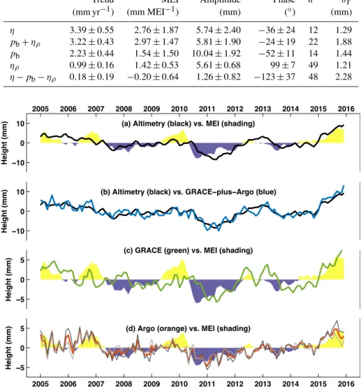
Figure 1a shows nonseasonal anomalies of GMSL (i.e., an-nual cycle and trend removed) alongside the Multivariate ENSO Index (MEI) (Wolter and Timlin, 1998) over 2005– 2015. As in earlier papers cited above, there is a tight rela-tion between GMSL and MEI curves, such that the GMSL is higher during El Niño periods and lower during La Niña periods. The Pearson product-moment correlation coefficient (hereafter simply referred to as the correlation) between these two records (0.73) is significant at the 95 % confidence level and suggests that approximately half of the nonseasonal anomalous GMSL variance over this period corresponds to ENSO. More generally, we observe that correlation between the nonseasonal GMSL and MEI anomalies is significant for all other 11-year periods during the altimeter record, as well as for the entire 23-year altimetric record itself (not shown).
Nonseasonal GMSL anomalies from satellite altimetry data are consistent with the sum of barystatic and steric com-ponents from GRACE and Argo (Fig. 1b). The correlations between GMSL from GRACE and Argo and from altime-try (0.89), and between MEI and the sum of GRACE and Argo (0.67), are both significant. Correlation values between GRACE and the MEI (0.54; Fig. 1c) and Argo and the MEI (0.65; Fig. 1d) are also significant. In fact, all pairs of time series displayed in Fig. 1 are significantly correlated (not shown). These results suggest that GMSL fluctuations tied to ENSO and seen by satellite altimetry are independently corroborated by the other ocean observing platforms and that barystatic and steric terms both contribute to the significant relationship between GMSL and ENSO.
Table 1.Results of OLS applied to altimetric GMSL (η), GRACE barystatic sea level (pb), Argo steric sea level (ηρ), and linear combinations
thereof. Values are given as 90 % confidence intervals as described in Appendix B. Note that, while the predictors of the OLS fit include an annual sine and cosine, we present results here transformed into the amplitude and phase of a sine term using standard trigonometric transformations. Note also thatn∗is the effective number of data points (evaluated following Eq. A3 in the Appendix), whereasδY is the
standard error evaluated for the different data as outlined in Sect. 2.
Trend MEI Amplitude Phase n∗ δY
(mm yr−1) (mm MEI−1) (mm) (◦) (mm)
η 3.39±0.55 2.76±1.87 5.74±2.40 −36±24 12 1.29 pb+ηρ 3.22±0.43 2.97±1.47 5.81±1.90 −24±19 22 1.88
pb 2.23±0.44 1.54±1.50 10.04±1.92 −52±11 14 1.44
ηρ 0.99±0.16 1.42±0.53 5.61±0.68 99±7 49 1.21
η−pb−ηρ 0.18±0.19 −0.20±0.64 1.26±0.82 −123±37 48 2.28
2005 2006 2007 2008 2009 2010 2011 2012 2013 2014 2015 2016
−10 0 10
Height (mm)
(a) Altimetry (black) vs. MEI (shading)
2005 2006 2007 2008 2009 2010 2011 2012 2013 2014 2015 2016
−10 0 10
Height (mm)
(b) Altimetry (black) vs. GRACE−plus−Argo (blue)
2005 2006 2007 2008 2009 2010 2011 2012 2013 2014 2015 2016
−5 0 5
Height (mm)
(c) GRACE (green) vs. MEI (shading)
2005 2006 2007 2008 2009 2010 2011 2012 2013 2014 2015 2016 −5
0 5
Height (mm)
(d) Argo (orange) vs. MEI (shading)
Figure 1.Monthly time series over 2005–2015 of(a)altimetric GMSL (black) and the MEI (shading),(b)GMSL from altimetry (black) and from GRACE and Argo (blue),(c)GRACE barystatic sea level (green) and the MEI (shading), and(d)Argo steric sea level (orange) and the MEI (shading). The thin dark gray (light gray) curve in(d)is Argo steric sea level based on the SIO (IPRC) gridded dataset. Linear trends and annual cycles have been removed from all time series. The MEI record has been scaled to have variance equal to that of the respective sea level time series.
of decadal trend, annual cycle, and MEI regressors, simul-taneously solving for the regression coefficients for all pre-dictors by minimizing the residual. This particular form of linear regression is motivated by previous studies referenced in the Introduction. (Indeed, the regression explains&90 % of the variance in the GMSL, barystatic, and steric curves over 2005–2015, and the coefficients of the regressors are all statistically significant, as revealed in Table 1 and discussed in more detail below, suggesting that this form of regression model is justified.) While OLS assumes the residuals behave as white noise, in practice we find that residuals are serially
correlated (not shown). Thus, we inflate the standard errors according to the lag-1 autocorrelation and the effective de-grees of freedom as detailed in Chambers et al. (2012) and Calafat and Chambers (2013). More technical details of our methods are found in Appendix A.
which is close to the value of 2.97±1.47 mm given by the sum of Argo steric and GRACE barystatic terms. Indeed, the residual value is not statistically distinguishable from zero (−0.20±0.64 mm), showing that the GMSL budget related to ENSO can be closed using observational data. Closure of the budget implies that steric contributions from regions not sampled by Argo (shelf seas, Arctic Ocean, below 2000 m) cannot be detected over the study period. Llovel et al. (2014) reach a similar conclusion regarding deep ocean steric contributions to the GMSL trend budget over 2005–2013. Significant regression coefficients are also determined for Argo steric (1.42±0.53 mm) and GRACE barystatic (1.54±1.50 mm) components. The error bars on the barystatic term are comparatively wider than on the steric term, agreeing with the relatively stronger correlation be-tween Argo and MEI than bebe-tween GRACE and MEI seen above (Fig. 1).
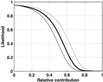
The OLS regression coefficients demonstrate that steric and barystatic effects generally make comparable contribu-tions to the ENSO-related GMSL changes over the study pe-riod. Judging from Monte Carlo simulations performed us-ing values in Table 1 (see Appendix D), it is as likely as not (33–66 % likelihood) that barystatic effects are respon-sible for 45–58 % of the sum of barystatic and steric contri-butions to GMSL variations linked to ENSO, and very un-likely (<10 % likelihood) that the barystatic term amounts to>68 % (Fig. 2). This is at odds with the emphasis placed on the barystatic contribution by recent studies (e.g., Llovel et al., 2011; Cazenave et al., 2012, 2014), revealing that, at least over this time period, the steric component is equally as important.
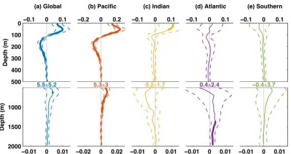
Regional distributions of ENSO-related terrestrial water storage, which are ultimately coupled to the barystatic con-tributions to GMSL fluctuations through mass conservation, are explored in past papers (Llovel et al., 2011; Boening et al., 2012; Phillips et al., 2012; Fasullo et al., 2013; de Linage et al., 2013; Eicker et al., 2016); they are not revisited here. However, ENSO-related GMSL behavior owing to steric ef-fects is not as well understood. The steric contributions to the GMSL fluctuations related to ENSO arise from changes in ocean heat content. Arguments based on mass conservation (Munk, 2003) suggest that any global steric contributions re-sulting from salinity changes would be exceedingly small. To elucidate ocean heat content changes potentially contribut-ing to GMSL changes related to ENSO, we apply the OLS method to Argo vertical potential temperature profiles, aver-aging horizontally over the global ocean as well as individual ocean basins (Fig. 3).
There is significant warming of the global ocean’s sur-face waters (0–100 m) and cooling within its main thermo-cline (130–320 m) during El Niño periods. Marginally signif-icant warming also occurs at some intermediate depths (600– 650 m). On the whole, the global upper ocean (0–2000 m) gains 5.5±5.2 ZJ (ZJ≡1021J) of heat per unit of MEI in-crease (equivalent to a uniform global ocean temperature
0 0.2 0.4 0.6 0.8 1
0 0.2 0.4 0.6 0.8 1
Relative contribution
Likelihood
Figure 2.The thick black curve is the likelihood that the barystatic contribution to ENSO-related GMSL changes will exceed a certain fraction of the sum of barystatic and steric terms based on Monte Carlo runs, where the steric term is evaluated based on the average of the SIO and IPRC gridded data products. The thin dark gray (light gray) curve is that same likelihood but with the steric term assessed using only the SIO (IPRC) product.
variation on the order of 0.001◦C). While there are some sig-nificant thermal changes related to ENSO observed in other basins at some depths (<60 m in the Indian; >1350 m in the Atlantic; see Fig. 3 caption for basin definitions), the vertical structure of the global ocean’s ENSO-related ther-mal variations derives from the Pacific, where there is simi-lar warming near the surface (0–110 m), cooling in the ther-mocline (130–320 m), and warming of intermediate waters (500–1150 m). Indeed, only the Pacific shows significant net thermal changes during ENSO, which is hardly surprising as ENSO originates from coupled air–sea interactions in the Pa-cific (e.g., Clarke, 2008, and references therein).
investi-−0.1 0 0.1 0
100
200
300
400
500
(a) Global
Depth (m)
5.5±5.2
−0.2 0 0.2 (b) Pacific
5.3±3
−0.1 0 0.1 (c) Indian
0.2±1.7
−0.1 0 0.1 (d) Atlantic
0.4±2.4
−0.1 0 0.1 (e) Southern
−0.4±3.7
−0.01 0 0.01 1000
1500
2000
Depth (m)
−0.02 0 0.02 −0.01 0 0.01 −0.01 0 0.01 −0.01 0 0.01
Figure 3.Coefficients of regressions of Argo potential temperature on the MEI (◦C per MEI) over 2005–2015 over(a)the global ocean and the(b)Pacific,(c)Indian,(d)Atlantic, and(e)Southern (south of 30◦S) basins. Solid lines are the regression coefficients and dashed lines mark the 90 % confidence interval. Bold lines mark significance at the 95 % confidence level (i.e., one-tailed test). Note the different horizontal axis limits between the top and bottom panels. The colored values between the top and bottom panels represent the total ocean heat storage (units of ZJ per MEI; 1 ZJ≡1021J) integrated over 0–2000 m in the different basins given as 90 % confidence intervals. For this figure, the Indian Ocean was defined as between 31.5 and 122.5◦E and north of 30.5◦S, the Atlantic Ocean between 76.5◦W and 14.5◦E and north of 30.5◦S, the Pacific Ocean between 118.5◦E and 69.5◦W and north of 30.5◦S, and the Southern Ocean south of 30.5◦S.
gate a longer time period and corroborate or refute the purely observational results presented here, but also to better under-stand the physical processes contributing to the global and regional steric changes (cf. Piecuch and Ponte, 2011, 2014).
Previous studies suggest that both the global ocean and climate system lose heat during El Niño events (e.g., Roem-mich and Gilson, 2011; Loeb et al., 2012; Trenberth et al., 2014). This would appear to conflict with our finding that the ocean is warmer during El Niños. However, the discrep-ancy is only apparent, since we consider ocean heat content and those past studies focus on the ocean heat content ten-dency (i.e., its rate of change). Moreover, scrutinizing visual examination of the earlier results (e.g., Fig. 8 in Trenberth et al., 2014) suggests that there is a phase lag between ENSO and the heat content tendency, such that warming precedes El Niño peaks and cooling follows peaks. This would be fully consistent with our findings, and those of von Schuckmann et al. (2014), who show a negative global ocean heat con-tent anomaly during the 2010–2011 La Niña. Future stud-ies should investigate in closer detail the coherence between variations in ocean heat content and ENSO.
The vertical structure of ocean temperature changes during ENSO events found here (Fig. 3) has implications for under-standing which ocean regions and depth levels contributed to the recent “surface warming slowdown”, which some partly relate to the dominant La Niña phase of the 2000s relative to the 1990s (Kosaka and Xie, 2013; Cazenave et al., 2014; England et al., 2014; Risbey et al, 2014). Nieves et al. (2015) determine that the slowdown was caused by a decadal shift
9.4$
5.3$
'5.8$
1.8$
4.1$
1.8$
Ocean$$ surface$
Main$$ thermocline$
Intermediate$$
waters
Figure 4.Hypothesized Pacific heat budget during El Niño events. The blue blocks are the ocean surface (0–110 m), main thermocline (120–380 m), and intermediate water (400–2000 m) layers. The red arrows are heat exchanges between the ocean layers or with the overlying atmosphere. Black values are either the total ocean heat storage within the layers as given by Argo data or the required heat exchanged between them under the stated assumptions of no transports between ocean basins and no contributions from the deep (>2000 m) ocean. Units are ZJ per unit MEI. (Note that all arrows and signs, shown here for El Niño, would be reversed for La Niña.)
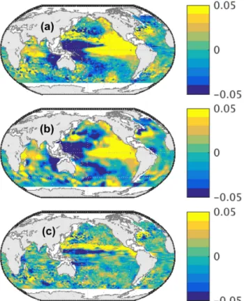
Figure 5. (a)Spatial pattern of nonseasonal anomalous Argo steric sea level (relative to 2005–2015 with linear trends and annual cy-cles removed) computed from the SIO gridded dataset over the last 6 months (July–December) of 2015. (b) As in(a)but computed from the IPRC gridded dataset.(c)Spatial pattern of the difference between the two gridded datasets (i.e., SIO minus IPRC). All panels have units of cm steric sea level.
300 m warmed from the 1990s to the 2000s, but that the rate of global ocean heat storage above 1500 m did not change during that time. Our results (Fig. 3) suggest that cooling of the surface Pacific between the 2 decades is consistent with phasing of ENSO, but subsurface Indian warming and lack of net ocean warming or cooling are not, hinting that processes unrelated to ENSO also contributed to the surface warming slowdown, consonant with papers showing an important role for the Interdecadal Pacific Oscillation (Meehl et al., 2013; Trenberth and Fasullo, 2013; Steinman et al., 2015; Fyfe et al., 2016).
In this study, SIO and IPRC Argo datasets were consid-ered. While reflected in the standard errors, differences be-tween these two products are apparent. For example, while both curves evidence an overall increase from the beginning of 2011 to the middle of 2015, the SIO and IPRC global steric height series diverge thereafter, with IPRC turning down and decreasing, and SIO continuing to rise through the latter half of 2015 (Fig. 1d). These global differences stem from regional discrepancies (Fig. 5). Nonseasonal steric height patterns over the global ocean from SIO and IPRC from July to December 2015 are generally similar, but
mani-fest clear discrepancies in the North Pacific, such that SIO shows more negative values than IPRC near the Equator towards the west, and more positive values over the trop-ics more broadly (Fig. 5c). Differences between the datasets could be due to different data sources, vertical resolution, or processing strategies, and more detailed future studies should more definitively attribute such discrepancies. Results shown in Llovel et al. (2014) attest to similar differences between SIO and IPRC datasets with regard to the global steric height trend over 2005–2013. Our qualitative conclusions are robust to such quantitative differences between the Argo datasets; for example, employing either SIO or IPRC only, the GMSL budget related to ENSO closes (not shown), and it is un-likely (<33 % likelihood) that the barystatic term contributes
>68 % to the sum of barystatic and thermosteric contribu-tions to the GMSL changes linked to ENSO (Fig. 2).
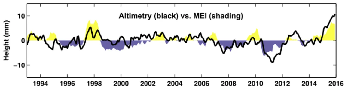
Finally, nonseasonal anomalous GMSL was considerably higher during the 2014–2015 El Niño than during the 1997– 1998 El Niño (Fig. 6), which is noteworthy because these two El Niño events were comparable in amplitude. (In addition to the distinct axis limits, Figs. 1a and 6 differ in that the re-moved linear trend and annual cycle are estimated for 2005– 2015 in the former and 1993–2015 in the latter.) This could suggest that the relationship between GMSL and ENSO is a complicated function of time period and frequency band, in which case the results presented here apply strictly to the study period. However, it could also suggest that other cli-mate modes (e.g., Pacific Decadal Oscillation, e.g., Hamling-ton et al., 2016) exert an influence on GMSL that has yet to be discussed.
4 Conclusions
grid-1994 1996 1998 2000 2002 2004 2006 2008 2010 2012 2014 2016
−10 0 10
Height (mm)
Altimetry (black) vs. MEI (shading)
Figure 6.Nonseasonal anomalies of GMSL (black) and MEI (shading) over 1993–2015.
ded Argo datasets (Fig. 5) and to determine why the anoma-lous GMSL response to ENSO was apparently much stronger during the 2014–2015 El Niño than during the 1997–1998 El Niño (Fig. 6). Our results corroborate previous suggestions made based on models (Landerer et al., 2008) or observa-tions during an isolated event (Dieng et al., 2014, 2015) that steric contributions to ENSO-related GMSL fluctuations are not negligible relative to barystatic contributions. These find-ings also have implications more generally for understanding the ocean’s role in the planet’s radiation imbalance and hy-drological cycle.
5 Data availability
Appendix A: Description of the OLS method
Let us regard the altimetric GMSL record (or any other data series for that matter)Y for 2005–2015 (including trend and annual cycle) as a linear combination of predictorsX:
Y =Xβ+ε. (A1)
HereXincludes the linear trend (slope and intercept), annual cycle (sine and cosine), and MEI,εis the error term, andβ
contains the regression coefficients to be solved for. The OLS estimator forβ is that vector which minimizes the variance betweenY andXβ,
ˆ
β=MY, (A2)
where M=. XTX−1
XT is the Moore–Penrose pseudo-inverse and Tis the matrix transpose. While OLS assumes white noise residuals, we find that εis autocorrelated (not shown). Thus, we assume a first-order autoregressive model, inflating the OLS standard errors by computing the lag-1 autocorrelation ϕ and finding the effective number of data pointsn∗,
n∗=n
1−ϕ
1+ϕ
, (A3)
where heren=132 months of observations over 2005–2015. This effective number of data points is then used for deter-mining the OLS standard error for the regression coefficients,
ˆ
σβˆj = s
εTε n∗−k
XTX
−1
jj, (A4)
whereβˆj is the jth coefficient andk=5 is the total
num-ber of coefficients being estimated. Similar methods are de-scribed by Chambers et al. (2012) and Calafat and Cham-bers (2013). Other methods are possible for linear estimation in the presence of autocorrelated residuals (e.g., feasible gen-eralized least squares), but we find that – in this context – these methods result in endogenous predictors (specifically, residuals of the fit are significantly correlated with the MEI predictor term), hence inconsistent estimates, and so are not employed.
Appendix B: Evaluation of 90 % confidence intervals All values derived from OLS regression quoted in the main text, shown in Fig. 3, and given in Table 1, are 90 % con-fidence intervals. These intervals are determined as follows. First, to account for goodness of fit, we compute the OLS standard errors, adjusting values according to the effective degrees of freedom, as above. Second, to account for uncer-tainty in the data, we propagate the standard errors in the data
based on the OLS estimator and the usual procedures for un-certainty propagation (e.g., Thomson and Emery, 2014),
δβˆj=δY
q MMT
jj, (B1)
where δY represents the standard error on the altimetry,
GRACE, or Argo data as outlined in the text and given in Table 1. We useσˆβˆ
j andδβˆj to evaluate the total uncertainty eβˆ
j, eβˆj=
r
ˆ
σ2ˆ
βj
+δ2ˆ
βj
. (B2)
Using these values for the total errors, the 90 % confidence intervals are constructed as
ˆ
βj−t95·eβˆj ≤βj≤ ˆβj+t95·eβˆj, (B3)
whereβj is the true value of thejth coefficient andt95is the ninety-fifth percentile of the Student’st inverse cumulative distribution given the effective degrees of freedom (Table 1).
Appendix C: Budgets for the annual cycle and linear trend
Here we briefly consider the GMSL budget for the annual cycle and the linear trend. These cases have been discussed before in many previous investigations (e.g., Leuliette, 2015, and references therein), and are discussed here mainly for the sake of completeness. Altimetry gives a GMSL trend over 2005–2015 of 3.39±0.55 mm yr−1, whereas the sum of GRACE and Argo yields 3.22±0.43 mm yr−1(Table 1). The residual between these two values 0.18±0.19 mm yr−1 is not statistically distinguishable from zero at the 95 % con-fidence level. We see that GRACE barystatic contributes roughly two-thirds to the total change (2.23±0.44 mm yr−1), whereas Argo steric contributes about one-third (0.99± 0.16 mm yr−1). The general closure of the budget and the rel-ative partitioning between barystatic and steric effects is very similar to other studies for similar periods (e.g., see Leuli-ette, 2015, for an assessment of the observed GMSL budget for 2005–2013).
Miller (2009) show a similar difference in GMSL phase be-tween altimetry and the sum of Argo and GRACE. It is not immediately obvious what is responsible for this discrep-ancy, and it is beyond our scope to explore the issue in depth. However, we hypothesize that it is due to sampling errors in the observing system, namely the fact that Argo does not sample at high latitudes or, probably more importantly, on shallow continental shelf seas.
Appendix D: Description of Monte Carlo simulation We evaluate what the likelihood is that the barystatic sea level term contributes more to ENSO-related GMSL fluctuations than the steric sea level term. We make this evaluation prob-abilistically, performing 100 000 iterations of drawing two values, each one drawn from a separate Student t distribu-tion. The first distribution is based on the MEI regression coefficient for the GRACE barystatic term, with location pa-rameter equal to the regression coefficient, scale papa-rameter equal to the standard error of the regression coefficient, and using the effective degrees of freedom. A draw from this first distribution is a possible value of the barystatic contribution. Likewise, the second distribution is based on the MEI regres-sion coefficient for the Argo steric term, with draws from this second distribution being possible values for the steric con-tribution. For each iteration, we assess the fraction,
F =D1(D1+D2) ,
where D1 and D2 are the draws from the first and second distributions, respectively. Physically,F represents the frac-tional barystatic contribution to the total GMSL change. The histogramP is derived from the realizations ofF. Figure 2 displays the likelihood,
L(x)=1−
x
Z
−∞
P (x′)dx′, (D1)
where L(x) is the probability (i.e., fraction of iterations) that F > x. For example, L(0.6)is the likelihood that the barystatic term is responsible for >60 % of total GMSL change.
Appendix E: Datasets E1 Satellite altimetry
The AVISO (Archiving, Validation, and Interpretation of Satellite Oceanographic data service) data were down-loaded from the AVISO website (Table E1). The data are based on reference missions (Ocean Topography Experiment (TOPEX)/Poseidon and Jason series) with inverted barom-eter correction applied, the seasonal signal retained, and glacial isostatic adjustment applied.
The CSIRO (Commonwealth Scientific and Industrial Re-search Organisation) data were downloaded from the CSIRO website (Table E1). The version of the data used here had the inverse barometer and glacial isostatic adjustment corrections applied and the seasonal signals not removed (“jb_iby_srn_gtn_giy”). A 60-day smoothing was used to re-duce a spurious 59-day cycle in the data related to alias of the ocean tides.
The Colorado data were downloaded from the Colorado sea level website (Table E1). The data version is ver-sion_2016rel2. A 60-day boxcar filter was also applied to the data.
The NOAA (National Oceanic and Atmospheric Adminis-tration) data were downloaded from the NOAA website (Ta-ble E1). The product used here is based on TOPEX/Poseidon and Jason series data with the seasonal signals retained. A 60-day smoothing was applied to these data and a trend of 0.3 mm yr−1 was added to account for glacial isostatic ad-justment effects not accounted for in this product.
E2 Profiling floats
The SIO Argo data were downloaded from the SIO website (Table E1). We used the 2004–2014 climatologies with the provided monthly extensions through February 2016.
The IPRC gridded data fields were downloaded from the IPRC website (see Table E1).
E3 Gravimetric retrievals
The GRACE data were downloaded from Don P. Chambers’ Dropbox folder (Table E1). Data gaps and missing months in these time series were filled based on cubic interpolation. E4 Climate indices
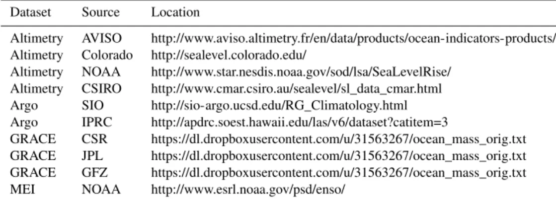
Table E1.Locations and sources of the data used here. Websites accessible as of 2 June 2016.
Dataset Source Location
Altimetry AVISO http://www.aviso.altimetry.fr/en/data/products/ocean-indicators-products/ Altimetry Colorado http://sealevel.colorado.edu/
Altimetry NOAA http://www.star.nesdis.noaa.gov/sod/lsa/SeaLevelRise/ Altimetry CSIRO http://www.cmar.csiro.au/sealevel/sl_data_cmar.html Argo SIO http://sio-argo.ucsd.edu/RG_Climatology.html Argo IPRC http://apdrc.soest.hawaii.edu/las/v6/dataset?catitem=3
Acknowledgements. Support for this research came from NASA grants NNX14AJ51G and NNH16CT00C. Helpful conversations with Steve Nerem, Rui Ponte, Don Chambers, and John Gilson are acknowledged. Two anonymous reviewers made valuable comments and suggestions, especially with respect to comparing the Argo datasets. The providers of the datasets are formally acknowledged in Appendix E and Table E1.
Edited by: M. Hoppema
Reviewed by: two anonymous referees
References
Ablain, M., Cazenave, A., Valladeau, G., and Guinehut, S.: A new assessment of the error budget of global mean sea level rate esti-mated by satellite altimetry over 1993–2008, Ocean Sci., 5, 193– 201, doi:10.5194/os-5-193-2009, 2009.
Bettadpur, S.: CSR Level-2 Processing Standards Document for Product Release 05 GRACE 327-742, revision 4.0, 2012 Boening, C., Willis, J. K.., Landerer, F. W., Nerem, R. S., and
Fa-sullo, J.: The 2011 La Niña: So strong, the oceans fell, Geophys. Res. Lett., 39, L19602, doi:10.1029/2012GL053055, 2012. Calafat, F. M. and Chambers, D. P.: Quantifying recent
accelera-tion in sea level unrelated to internal climate variability, Geo-phys. Res. Lett., 40, 3661–3666, 2013
Calafat, F. M., Chambers, D. P., and Tsimplis, M. N.: On the ability of global sea level reconstructions to determine trends and variability, J. Geophys. Res.-Oceans, 119, 1572–1592, doi:10.1002/2013JC009298, 2014.
Cazenave, A., Dominh, K., Guinehut, S., Berthier, E., Llovel, W., Ramillien, G., Ablain, M., and Lamicol, G.: Sea level budget over 2003–2008: A reevaluation from GRACE space gravimetry, satellite altimetry and Argo, Global Planet. Change, 65, 83–88, 2009.
Cazenave, A., Henry, O., Munier, S., Delcroix, T., Gordon, A. L., Meyssignac, B., Llovel, W., Palanisamy, H., and Becker, M.: Es-timating ENSO Influence on the Global Mean Sea Level, 1993– 2010, Mar. Geod., 35, 82–97, 2012.
Cazenave, A., Dieng, H.-B., Meyssignac, B., von Schuckmann, K., Decharme, B., and Berthier, E.: The rate of sea-level rise, Nature Climate Change, 4, 358–361, 2014.
Chambers, D. P. and Bonin, J. A.: Evaluation of Release-05 GRACE time-variable gravity coefficients over the ocean, Ocean Sci., 8, 859–868, doi:10.5194/os-8-859-2012, 2012.
Chambers, D. P., Mehlhaff, C. A., Urban, T. J., Fujii, D., and Nerem, R. S.: Low-frequency variations in global mean sea level: 1950–2000, J. Geophys. Res., 107, C43026, doi:10.1029/2001JC001089, 2002.
Chambers, D. P., Merrifield, M. A., and Nerem, R. S.: Is there a 60-year oscillation in global mean sea level?, Geophys. Res. Lett., 39, L18607, doi:10.1029/2012GL052885, 2012.
Church, J. A. and White, N. J.: Sea-Level Rise from the Late 19th to the Early 21st Century, Surv. Geophys., 32, 585–602, 2011. Clarke, A. J.: An Introduction to the Dynamics of El Nino & the
Southern Oscillation, Academic Press, 324 pp., 2008.
de Linage, C., Kim, H., Famiglietti, J. S., and Yu, J.-Y.: Impact of Pacific and Atlantic sea surface temperatures on interannual and decadal variations of GRACE land water storage in
tropi-cal South America, J. Geophys. Res. Atmos., 118, 10811–10829, 2013.
Dahle, C.: GFZ Level-2 Processing Standards Document for Prod-uct Release 05 GRACE 327-742, revision 1.1, 2013.
Dieng, H. B., Cazenave, A., Meyssignac, B., Henry, O., von Schuckmann, K., Palanisamy, H., and Lemoine, J. M.: Effect of La Niña on the global mean sea level and north Pacific ocean mass over 2005–2011, J. Geod. Sci., 4, 19–27, 2014.
Dieng, H. B., Palanisamy, H., Cazenave, A., Meyssignac, B., and von Schuckmann, K.: The Sea Level Budget Since 2003: Infer-ence on the Deep Ocean Heat Content, Surv. Geophys., 36, 2, 209–229, doi:10.1007/s10712-015-9314-6, 2015.
Eicker, A., Forootan, E., Springer, A., Longuevergne, L., and Kusche, J.: Does GRACE see the terrestrial water cycle “intensi-fying”?, J. Geophys. Res. Atmos., 121, 733–745, 2016. England, M. H., McGregor, S., Spence, P., Meehl, G. A.,
Timmer-mann, A., Cai, W., Sen Gupta, A., McPhaden, M. J., Purich, A., and Santoso, A.: Recent intensification of wind-driven circula-tion in the Pacific and the ongoing warming hiatus, Nature Cli-mate Change, 4, 222–227, 2014.
Fasullo, J. T., Boening, C., Landerer, F. W., and Nerem, R. S.: Aus-tralia’s unique influence on global sea level in 2010–2011, Geo-phys. Res. Lett., 40, 4368–4373, 2013.
Forget, G., Campin, J.-M., Heimbach, P., Hill, C. N., Ponte, R. M., and Wunsch, C.: ECCO version 4: an integrated framework for non-linear inverse modeling and global ocean state estimation, Geosci. Model Dev., 8, 3071–3104, doi:10.5194/gmd-8-3071-2015, 2015.
Fyfe, J. C., Meehl, G. A., England, M. H., Mann, M. E., Santer, B. D., Flato, G. M., Hawkins, E., Gillett, N. P., Xie, S.-P., Kosaka, Y., and Swart, N. C.: Making sense of the early-2000s warming slowdown, Nature Climate Change, 6, 224–228, 2016.
Gill, A. E. and Niiler, P. P.: The theory of the seasonal variability in the ocean, Deep-Sea Res., 20, 141–177, 1973.
Gregory, J. M., White, N. J., Church, J. A., Bierkens, M. F. P., Box, J. E., van den Broeke, M. R., Cogley, J. G., Fettweis, X., Hanna, E., Huybrechts, P., Konikow, L. F., Leclercq, P. W., Marzeion, B., Oerlemans, J., Tamisiea, M. E., Wada, Y., Wake, L. M., and van de Wal, R. S. W.: Twentieth-Century Global-Mean Sea Level Rise: Is the Whole Greater than the Sum of the Parts? J. Clim., 26, 4476–4499, 2013.
Haddad, M., Taibi, H., and Areski, S. M. M.: On the recent global mean sea level changes: Trend extraction and El Niño’s impact, C. R. Geosci., 345, 167–175, 2013.
Hamlington, B. D., Cheon, S. H., Thompson, P. R., Merrifield, M. A., Nerem, R. S., Leben, R. R., and Kim, K.-Y.: An ongoing shift in Pacific Ocean sea level, J. Geophys. Res.-Oceans, 121, 5084– 5097, doi:10.1002/2016JC011815, 2016.
Johnson, G. C. and Chambers, D. P.: Ocean bottom pressure sea-sonal cycles and decadal trends from GRACE Release-05: Ocean circulation implications, J. Geophys. Res.-Oceans, 118, 4228– 4240, 2013.
Kosaka, Y. and Xie, S.-P.: Recent global-warming hiatus tied to equatorial Pacific surface cooling, Nature, 501, 403–407, 2013. Landerer, F. W., Jungclaus, J. H., and Marotzke, J.: El
Leuliette, E.: The Budget of Recent Global Sea Level Rise 2005– 2013, NOAA NESDID Report, 10 pp., 2014.
Leuliette, E. W.: The Balancing of the Sea-Level Budget, Curr. Clim. Change Rep., 1, 185–191, 2015.
Leuliette, E. W. and Miller, L.: Closing the sea level rise budget with altimetry, Argo, and GRACE, Geophys. Res. Lett., 36, L04608, doi:10.1029/2008GL036010, 2009.
Leuliette, E. W. and Scharroo, R.: Integrating Jason-2 into a multiple-altimeter climate data record, Mar. Geod., 33, 504, doi:10.1080/01490419.2010.487795, 2010.
Leuliette, E. W. and Willis, J. K.: Balancing the sea level budget, Oceanography, 24, 2, 122–129, 2011.
Llovel, W., Becker, M., Cazenave, A., Crétaux, J.-F., and Ramillien, G.: Global land water storage change from GRACE over 2002– 2009; Inference on sea level, C. R. Geosci., 342, 179–188, 2010. Llovel, W., Becker, M., Cazenave, A., Jevrejeva, S., Alkama, R., Decharme, B., Douville, H., Ablain, M., and Beckley, B.: Ter-restrial waters and sea level variations on interannual time scale, Global Planet. Change, 75, 76–82, 2011.
Llovel, W., Willis, J. K., Landerer, F. W., and Fukumori, I.: Deep-ocean contribution to sea level and energy budget not detectable over the past decade, Nature Climate Change, 4, 1031–1035, 2014.
Loeb, N. G., Lyman, J. M., Johnson, G. C., Allan, R. P., Doelling, D. R., Wong, T., Soden, B. J., and Stephens, G. L.: Observed changes in top-of-the-atmosphere radiation and upper-ocean heating consistent within uncertainty, Nat. Geosci., 5, 110–113, 2012.
Lombard, A., Garcia, D., Ramillien, G., Cazenave, A., Biancale, R., Lemoine, J. M., Flechtner, F., Schmidt, R., and Ishii, M.: Estima-tion of steric sea level variaEstima-tions from combined GRACE and Jason-1 data, Earth Planet Sc. Lett., 254, 194–202, 2007. Masters, D., Nerem, R. S., Choe, C., Leuliette, E., Beckley, B.,
White, N., and Ablain, M.: Comparison of Global Mean Sea Level Time Series from TOPEX/Poseidon, 1, and Jason-2, Mar. Geod., 35, 20–41, 2012.
Mayer, M., Haimberger, L., and Balmaseda, M. A.: On the Energy Exchange between Tropical Ocean Basins Related to ENSO, J. Clim., 27, 6393–6403, 2014.
Meehl, G. A., Hu, A., Arblaster, J. M., Fasullo, J., and Trenberth, K. E.: Externally Forced and Internally Generated Decadal Climate Variability Associated with the Interdecadal Pacific Oscillation, J. Clim., 26, 7298–7310, 2013.
Merrifield, M. A., Nerem, R. S., Mitchum, G. T., Miller, L., Leuli-ette, E., Gill, S., and Woodworth, P. L.: Sea level variations, 2008 annual assessment, in: State of the Climate in 2008, edited by: Peterson, T. C. and Baringer, M. O., 2009.
Meyssignac, B. and Cazenave, A.: Sea level: A review of present-day and recent-past changes and variability, J. Geodynam., 58, 96–109, 2012.
Meyssignac, B., Lemoine, J. M., Cheng, M., Cazenave, A., Gé-gout, P., and Maisongrande, P.: Interannual variations in degree-2 Earth’s gravity coefficients C2, 0, C2, 2, and S2, 2 reveal large-scale mass transfers of climatic origin, Geophys. Res. Lett., 40, 4060–4065, 2013.
Munk, W.: Ocean Freshening, Sea Level Rising, Science, 300, 2041–2043. 2003.
Nerem, R. S., Chambers, D. P., Leuliette, E. W., Mitchum, G. T., and Giese, B. S.: Variations in global mean sea level associated
with the 1997–1998 ENSO event: Implications for measuring long term sea level change, Geophys. Res. Lett., 26, 19, 3005– 3008, 1999.
Nerem, R. S., Chambers, D. P., Choe, C., and Mitchum, G. T.: Es-timating Mean Sea Level Change from the TOPEX and Jason Altimeter Missions, Mar. Geod., 33, 435–446, 2010.
Ngo-Duc, T., Laval, K., Polcher, J., and Cazenave, A.: Contribu-tion of continental water to sea level variaContribu-tions during the 1997– 1998 El Niño-Southern Oscillation event: Comparison between Atmospheric Model Intercomparison Project simulations and TOPEX/Poseidon satellite data, J. Geophys. Res., 110, D09103, doi:10.29/2004JD004940, 2005.
Nieves, V., Willis, J. K., and Patzert, W. C.: Recent hiatus caused by decadal shift in Indo-Pacific heating, Science, 349, 532–536, 2015.
Phillips, T., Nerem, R., Fox-Kemper, B., Famiglietti, J., and Ra-jagopalan, B.: The influence of ENSO on global terrestrial wa-ter storage using GRACE, Geophys. Res. Lett., 39, L16705, doi:10.1029/2012GL052495, 2012.
Piecuch, C. G. and Ponte, R. M.: Mechanisms of interannual steric sea level variability, Geophys. Res. Lett., 38, L15605, doi:10.1029/2011GL048440, 2011.
Piecuch, C. G. and Ponte, R. M.: Mechanisms of Global-Mean Steric Sea Level Change, J. Clim., 27, 824–834, 2014.
Ponte, R. M. and Dorandeu, J.: Uncertainties in ECMWF Surface Pressure Fields over the Ocean in Relation to Sea Level Analyses and Modeling, J. Atmos. Ocean. Tech., 20, 301–307, 2003. Pugh, D. and Woodworth, P.: Sea-Level Science: Understanding
Tides, Surges, Tsunamis and Mean Sea-Level Changes, Cam-bridge University Press, 395 pp., 2014.
Risbey, J. S., Lewandowsky, S., Langlais, C., Monselesan, D. P., O’Kane, T. J., and Oreskes, N.: Well-estimated global surface warming in climate projections selected for ENSO phase, Nature Climate Change, 4, 835–840, 2014.
Roemmich, D. and Gilson, J.: The 2004–2008 mean and annual cy-cle of temperature, salinity, and steric height in the global ocean from the Argo program, Prog. Oceanogr., 82, 81–100, 2009. Roemmich, D. and Gilson, J.: The global ocean imprint of ENSO,
Geophys. Res. Lett., 38, L13606, doi:10.1029/2011GL047992, 2011.
Stammer, D., Cazenave, A., Ponte, R. M., and Tamisiea, M. E.: Causes for Contemporary Regional Sea Level Changes, Annu. Rev. Mar. Sci., 5, 21–46, 2013.
Steinman, B. A., Mann, M. E., and Miller, S. K.: Atlantic and Pa-cific multidecadal oscillations and Northern Hemisphere temper-atures, Science, 347, 988–992, 2015.
Tapley, B. D., Bettadpur, S., Watkins, M. and Reigber, C.: The gravity recovery and climate experiment: Mission overview and early results, Geophys. Res. Lett., 31, L09607, doi:10.1029/2004GL019920, 2004.
Thomson, R. E. and Emery, W. J.: Data Analysis Methods in Phys-ical Oceanography, Third Edition, Elsevier, 716 pp., 2014. Trenberth, K. E. and Fasullo, J. T.: An apparent hiatus in global
warming?, Earth’s Future, 1, 19–32, 2013.
Trenberth, K. E., Fasullo, J. T., and Balmaseda, M. A.: Earth’s En-ergy Imbalance, J. Clim., 27, 3129–3144, 2014.
Argo perspective, Ocean Sci., 10, 547–557, doi:10.5194/os-10-547-2014, 2014.
Watkins, M. and Yuan, D.: JPL Level-2 Processing Standards Doc-ument for Product Release 05 GRACE 327-742, revision 5.0, 2012.
Willis, J. K., Chambers, D. P., and Nerem, R. S.: Assess-ing the globally averaged sea level budget on seasonal to interannual timscales, J. Geophys. Res., 113, C06015, doi:10.1029/2007JC004517, 2008.