www.ocean-sci.net/12/647/2016/ doi:10.5194/os-12-647-2016
© Author(s) 2016. CC Attribution 3.0 License.
Analyses of altimetry errors using Argo and GRACE data
Jean-François Legeais, Pierre Prandi, and Stéphanie Guinehut
Collecte Localisation Satellites, Parc Technologique du canal, 8–10 rue Hermès, 31520 Ramonville Saint-Agne, France Correspondence to:Jean-François Legeais (jlegeais@cls.fr)
Received: 18 December 2015 – Published in Ocean Sci. Discuss.: 18 January 2016 Revised: 4 April 2016 – Accepted: 13 April 2016 – Published: 13 May 2016
Abstract. This study presents the evaluation of the perfor-mances of satellite altimeter missions by comparing the al-timeter sea surface heights with in situ dynamic heights de-rived from vertical temperature and salinity profiles mea-sured by Argo floats. The two objectives of this approach are the detection of altimeter drift and the estimation of the impact of new altimeter standards that requires an indepen-dent reference. This external assessment method contributes to altimeter calibration–validation analyses that cover a wide range of activities. Among them, several examples are given to illustrate the usefulness of this approach, separating the analyses of the long-term evolution of the mean sea level and its variability, at global and regional scales and results obtained via relative and absolute comparisons. The latter requires the use of the ocean mass contribution to the sea level derived from Gravity Recovery and Climate Experi-ment (GRACE) measureExperi-ments. Our analyses cover the es-timation of the global mean sea level trend, the validation of multi-missions altimeter products as well as the assessment of orbit solutions.
Even if this approach contributes to the altimeter quality assessment, the differences between two versions of altime-ter standards are getting smaller and smaller and it is thus more difficult to detect their impact. It is therefore essen-tial to characterize the errors of the method, which is illus-trated with the results of sensitivity analyses to different pa-rameters. This includes the format of the altimeter data, the method of collocation, the temporal reference period and the processing of the ocean mass solutions from GRACE. We also assess the impact of the temporal and spatial sampling of Argo floats, the choice of the reference depth of the in situ profiles and the importance of the deep steric contribution. These analyses provide an estimation of the robustness of the method and the characterization of associated errors. The results also allow us to draw some recommendations to the
Argo community regarding the maintenance of the in situ network.
1 Introduction
Since the early 1990s, several satellite missions have been equipped with altimeters allowing the estimation of sea level anomalies (SLAs) and the monitoring of mean sea level (MSL). This contributes to understanding the role of the ocean in the Earth system and to assess the link with the global climate change. Altimeters are available on-board several missions currently in flight (Jason-2 and 3, SARAL/AltiKa, CryoSat-2, Sentinel-3A, HY-2A) and those no longer providing data (TOPEX/Poseidon-T/P-, ERS-1 and 2, Jason-1, Envisat, Geosat Follow-On). Although sea level estimates are becoming more precise, there are still some uncertainties that can be distinguished at different tem-poral scales (long-term trend, interannual signals and peri-odic signals) both at global and regional scales (Ablain et al., 2015). The major sources of errors are attributed to or-bit solutions, instrumental corrections and some geophysical altimeter corrections such as the wet troposphere correction (Ablain et al., 2009; Couhert et al., 2014; Legeais et al., 2014; Rudenko et al., 2014).
coastal areas are sampled and the instruments are not homo-geneously distributed over the coasts (hemispheric bias).
In this study, we use dynamic height anomalies (DHAs) derived from the temperature and salinity (T/S) vertical pro-files of the Argo network. The Lagrangian profiling floats provide an almost global coverage of the open ocean with measurements from the surface to around 2000 dbar for most of them and the objective of a global network of 3000 operat-ing floats has been achieved in 2007 (Roemmich and Team, 2009). Taking advantage of the consistency between these in situ measurements and altimeter SLAs (Guinehut et al., 2006; Dhomps et al., 2011), several examples illustrate the usefulness of the comparison between these data in order to reach two major objectives in terms of calibration and vali-dation of altimeter data.
The first objective deals with the detection of drifts and jumps in the altimeter sea level time series. For instance, at global scale, the MSL trends of the Envisat and Jason-1 missions differ by 1.0 mm yr−1over the period 2004–2011 (Prandi et al., 2013). The absolute comparison of both al-timeter MSLs with Argo and Gravity Recovery and Climate Experiment (GRACE) measurements indicates that the MSL drift is greater for the Envisat than for the Jason-1 mission with a 1.4 mm yr−1 difference, which is confirmed by the 0.9 mm yr−1difference provided by the altimeter comparison with tide gauges measurements over the same period (Prandi et al., 2013). The use of in situ data as a reference allows for the detection and identification of the origin of global al-timeter MSL trend discrepancy between two missions that cannot be addressed by internal comparison only. Note that this Envisat drift is well known (Ollivier et al., 2012) and is no more observed with the use of the Envisat reprocessed measurements which have made both altimeter trends more homogeneous.
The second objective is to assess the potential improve-ment provided by a new altimeter standard (e.g., orbit solu-tion, geophysical corrections) in the SLA estimation (or new altimeter product), regarding the long-term evolution of the mean sea level or its variability, at global or regional scales, thanks to relative or absolute comparisons. A first example is provided by the regional eastern/western hemispheric bias observed in the spatial distribution of the Jason-1 MSL trends with the use of the GDR-D orbit solution (Legeais et al., 2015b). As Argo measurements are considered to be free of this regional anomaly, the relative comparison of the MSL trend differences between SLAs and DHA (computed in two different east/west regions where the greatest differences are observed) illustrates the strong regional discrepancy obtained with the GDR-D orbit solution (Fig. 1a: 2.3 mm yr−1). The use of the updated GDR-E orbit solution in the Jason-1 MSL calculation leads to a significant reduction of the regional dis-crepancies of the MSL trends (Fig. 1b, right: 0.1 mm yr−1), which demonstrates the better quality of this new altimeter standard. As discussed in Valladeau et al. (2012), the global Argo measurements are the only in situ external reference
Table 1.Statistics (correlation computed with a 95 % confidence interval) between altimeter products and in situ DHA with an ho-mogeneous reference period of the altimeter SLA and in situ DHA (2003–2011) in the Bay of Bengal (−5◦S/+20◦N; 80◦E/95◦E), Argo DHAs are referenced to 1900 dbar.
Argo DHA 1900 dbar Correlation rms of the differences (cm)
SSALTO/DUACS DT 2010 0.89 3.94 SSALTO/DUACS DT 2014 0.90 3.76
that allows us to discriminate such an impact regarding the altimeter MSL. Second, the independent Argo sea level es-timations can be used at global scale, by relative compari-son and in terms of MSL variability to distinguish between two different altimeter products such as the climate-oriented SL_cci v1.1 ECV product (Cazenave et al., 2014a; Ablain et al., 2015) and the 2014 SSALTO (Segment Sol Altime-trie et Orbitographie)/DUACS (Developing Use of Altimetry for Climate Studies) time series (AVISO, 2014; Pujol et al., 2016). This is illustrated in Fig. 2 (with triangles and circles, respectively) thanks to the Taylor diagram formalism (Tay-lor, 2001). Different frequencies of the differences between SLAs and DHA are distinguished (total signals in black, an-nual cycles in green, high frequencies in red and interanan-nual signals in blue) and such a diagram provides a way of graph-ically summarizing how closely different signals match ob-servations (in situ data: gray dot on the bottom axis) in terms of their correlation, their centered root-mean-square differ-ence and the ratio of their variances. Both altimeter prod-ucts have an annual cycle highly correlated with the in situ reference (in green), which has to be removed before ana-lyzing others signals. The diagram reveals that the products cannot be significantly distinguished regarding the total sig-nals (in black), their annual cycle (in green) and their high frequencies (in red). At low frequencies (in blue), the SL_cci product (triangle) is more in agreement with in situ data than the SSALTO/DUACS product (circle). As the quality of cli-mate products is better addressed at these low frequencies (inter-annual and long-term evolution of the sea level), this highlights the advantage of the SL_cci products for climate studies. However, the correlations of each altimeter data with the in situ reference are similar.
Figure 1.SSH differences (cm) between Jason-1 altimeter data (cycles 1 to 355) and Argo in situ measurements (900 dbar) computed with GDR-D(a)and GDR-E orbit solution(b), separating east box (Long: 60◦/120◦, Lat:−30◦/+30◦, in red) and west box (Long:−150◦/−190◦, Lat:−50◦/10◦, in blue). Corresponding annual and semi-annual signals are removed. Trends of raw data (dots) are indicated and the 2-month filtered signal is added (curves).
Figure 2.Taylor diagram of the comparison of SL_cci (triangles) and AVISO SSALTO/DUACS DT (circles) merged altimeter sea level products with Argo (900 dbar) and GRACE independent mea-surements for the global data (black) and separating high frequen-cies (red), the annual signal (green) and the inter-annual signals (blue).
All these illustrations clearly demonstrate that the Argo in situ measurements are a valuable tool to detect altimeter drift and to assess the impact of a new altimeter standard or product, regarding the long-term evolution of the mean sea level or its variability, at global or regional scales. How-ever, the evolutions provided by the new algorithms, allow-ing for the sea level calculation (orbit solution, instrumen-tal corrections, geophysical corrections, mean sea surface),
become more and more difficult to assess (Stammer et al., 2014; Fernandes et al., 2015; Couhert et al., 2014). Hence, it is essential to determine to which extent the comparison with Argo independent measurements can be used to con-tribute to the quality assessment of these new algorithms and thus to better characterize the remaining errors of the method of comparison and its sensitivity to the various parameters. Following the description of the different data sets used in our study (Sect. 2), sensitivity analyses of the method to dif-ferent parameters are presented. This includes the format of the altimeter data, the method of collocation, the temporal reference period and the processing of the ocean mass solu-tions from GRACE. We also assess the impact of the tem-poral and spatial sampling of Argo floats, the choice of the reference depth of the in situ profiles and the importance of the deep steric contribution. At last, concluding remarks are provided on the method uncertainty and the results also allow us to draw some recommendations for the Argo community regarding the maintenance of the in situ network.
2 Data sets 2.1 Altimetry
altimeter missions are computed with a reference to the mean sea surface (MSS) CNES (French national centre for space research)/CLS11 (Collecte Localisation Satellites) model (Schaeffer et al., 2012). Grids of merged altimeter products (level 4) are also compared with in situ data.
2.2 Argo
In this study, we use delayed mode and real-time quality-controlled T/S profiles (Guinehut et al., 2009) from the Coriolis Global Data Assembly Center (www.coriolis.eu.org; CORIOLIS, 2015). Following Roemmich and Gilson (2009), considering a threshold of two-thirds of the surface of the global open ocean covered by Argo floats, analyses should be performed with in situ data dating only from 2005 on-wards. This is a relevant reference for the latest altime-ter missions (Envisat, Jason-1, Jason-2, Jason-3, SARAL-AltiKa and Sentinel-3A) and results in an in situ data set of more than 10 000 floats with about 900 000T/Sprofiles dis-tributed over almost the whole open ocean. DHAs are com-puted as follows: dynamic heights are first comcom-puted from the integration of the Argo pressure, temperature and salinity vertical profiles using a reference depth. In order to calcu-late anomalies of dynamic heights consistent with altimeter SLAs, a mean dynamic height is used as a reference. It is es-timated through a synthetic climatology approach (Guinehut et al., 2006): the technique consists in combining altimeter SLAs with simultaneous in situ dynamic height to estimate the mean dynamic height. The choice of the reference level is discussed in this paper.
2.3 GRACE
Altimeter measurements are representative of the total ele-vation of the sea surface (surface to bottom), that includes barotropic and baroclinic components. DHAs from Argo pro-filing floats are representative of the steric elevation asso-ciated with the expansion and contraction of the water col-umn from the surface to the reference level of integration (i.e., baroclinic component) (Dhomps et al., 2011). As de-scribed in the previous section, the relative comparison be-tween altimeter SLAs and in situ DHAs is sufficient to detect an anomaly between two different altimeter missions or the impact of a new altimeter standard in the SLA calculation. However, the analysis of the absolute altimeter drift and bias requires the addition of the ocean mass contribution to the sea level, which is not included in the in situ measurements. This contribution is derived from the GRACE satellite mission. It provides a series of Earth gravity fields in the form of trun-cated sets of spherical harmonic (SH) coefficients (Stokes) at approximately monthly intervals (Tapley et al., 2004). Their temporal variations can be used to estimate changes in the ocean mass distribution in terms of equivalent water thick-ness (Chambers et al., 2004; Llovel et al., 2014; Ponte et al., 2007). As the total mass of the Earth is assumed to be
un-changed, the time-variable mean ocean mass is related to the exchanges of water mass with the continents and the atmo-sphere. These exchanges significantly contribute to the in-terannual evolution of the global MSL (Fasullo et al., 2013; Cazenave et al., 2014b). In this study, two ocean mass solu-tions are used: the monthly grids of equivalent water height from the Groupe de Recherche en Geodesie Spatiale (GRGS RL03v1; Biancale et al., 2014) and the global mean ocean mass time series from GRACE RL05, as provided by the University of South Florida – Satellite Oceanography Lab-oratory (available at: http://xena.marine.usf.edu/~chambers/ SatLab/Home.html) and described in Johnson and Cham-bers (2013).
3 Sensitivity of the method
This section focuses on the determination of the errors of the method of comparison of altimetry with Argo and GRACE data and provides sensitivity analyses of the method to differ-ent parameters. For each analysis, the impact of a parameter is estimated regarding the long-term evolution of the mean sea level or its variability at global or regional scales. In the following, the term “error” is considered as a quantity that would be removed if it was known whereas the term “un-certainty” is associated with the confidence that it can be at-tributed to the estimation of a given parameter. The fit un-certainty provided with the long-term trend estimations can be considered as a standard error: the confidence interval is 1 standard deviation of the statistical distribution of the trend estimators. In addition, comparisons of altimeter SLAs with in situ DHAs suffer from systematic errors. However, their realizations are the same when the SLA–DHA differences are analyzed by relative comparisons (for instance with the use of a new and reference altimeter standards in the SLA calculation or successively in two different hemispheres). In this case, these errors cancel each other, which make it pos-sible to detect some trend differences.
3.1 Format of altimeter data
Figure 3. Histogram of the difference of variance of the SLA–DHA differences for each Argo float using successively 1◦×1◦ vs. 1◦×3◦ boxes (i.e., Variance(SLA_1x1-DHA) – Variance(SLA_1x3-DHA)) when averaging along-track Jason-1 al-timeter SLAs before collocating with Argo profiles.
and phase of the annual signal of the SLA–DHA differences are not affected by this change of box size, neither is the trend of the differences (not shown).
The variance of the SLA–DHA differences is computed for the time series of each Argo floats, using successively the two different sizes of boxes for altimetry. The histogram of the difference of these variances for all Argo floats (Fig. 3) provides a mean of+1.3 cm2, which indicates that averaging
along-track altimeter data with 1◦×3◦boxes makes
altime-ter data more coherent with in situ Argo observations. This processing is therefore chosen for the comparisons.
3.2 Error of collocation
In order to improve the correlation between both types of data (and thus increase the accuracy of the results), outliers (corresponding to differences between altimeter SLAs and in situ DHA greater than 0.20 m) are filtered out. All asso-ciated measurements are located in regions of high ocean variability, which is expected given the method of colloca-tion of both types of data. In these regions, the time of two co-located altimeter and in situ measurements may not be strictly the same and the associated impact may be higher as the ocean state may change significantly within less than 10 days. Note that this effect could be reduced by computing maps of altimeter measurements by optimal interpolation. However, this is very time consuming since a set of grids has to be computed for a specific mission as soon as the impact of a new altimeter standard has to be evaluated.
In order to estimate the error of the method associated with these regions of high ocean variability, the compari-son of altimeter data with Argo measurements could be per-formed after removing areas where the ocean variability is higher than a given threshold. In terms of spatial coverage,
the lower this threshold is, the larger the areas removed. The detection of altimeter drift is not affected by the exclusion of areas of high ocean variability. Indeed, the 2.07 mm yr−1
trend of the mean differences between SSALTO/DUACS and Argo DHA (900 dbar reference) is not significantly changed when areas of ocean variability higher than 100 cm2are ex-cluded (2.16 mm yr−1). This will be confirmed with results described later in this paper regarding the sensitivity to the spatial sampling of the Argo network. Figure 4 (left) illus-trates that the lower the threshold on the ocean variability, the larger areas are removed and thus, a lower number of ob-servations are available. The right panel indicates that when larger areas are removed, the correlation between altimeter SLAs and Argo DHAs gets lower and the rms of the differ-ences (expressed in percentage of the altimeter variance) in-creases. This indicates that, contrary to the trend of the SLA– DHA differences, which is less sensitive, the global statistics computed between altimetry and Argo data are significantly affected by the areas of large ocean variability. However, this does not allow us to determine whether an increased sam-pling of these regions by the Argo network would improve the results of altimetry validation.
In addition, our study focuses on the altimeter quality as-sessment. In particular, the estimation of the global altimeter MSL drift is not considered to be significantly affected by the fact that some regions of the ocean are not covered by the Argo network (e.g., the Indonesian throughflow, the Gulf of Mexico). The steric contributions of such regions may be of importance for sea level closure budget studies (Dieng et al., 2015b), but similarly with comparisons to tide gauges, they do not prevent from estimating the global MSL evolution.
3.3 Impact of the temporal reference period
Figure 4.Impact of excluding areas of higher ocean variability than a decreasing threshold: number of observed points (left) and correlation and rms of the differences between AVISO DUACS 2014 and Argo DHAs (900 dbar reference) (right).
Table 2. Global correlation (with a 95 % confidence interval) be-tween all collocated altimeter SLAs (AVISO SSALTO/DUACS, 2010 and 2014; Pujol et al., 2016) and in situ DHAs from Argo pro-files (with a reference depth of 1900 dbar and a 2003–2011 temporal reference) without and with an homogeneous temporal reference.
Global correlation Non-homogeneous Homogeneous temporal reference temporal
reference AVISO SSALTO/DUACS (2010) 0.87 0.90 AVISO SSALTO/DUACS (2014) 0.90 0.90
of error of the method of comparison (different temporal ref-erences) that can be corrected (by referencing both data sets on the same period).
3.4 Impact of the GRACE data set and associated errors
At regional scales and particularly in the tropical ocean, total altimeter and steric annual signals are in phase (Dhomps et al., 2011; Legeais et al., 2015a) but due to the spatial distri-bution of the ocean on the Earth and seasonal hemispheric signals, the global time series are affected by a quadratic phase shift (Fig. 5 and Chen et al., 1998). Regarding the ocean mass contribution to the sea level, its annual signal has a larger magnitude (twice) than total and steric signals and is in phase with the total altimeter global MSL (Fig. 5). In addition, Fig. 6 highlights that the amplitude of the annual signal of the global differences between the total altimeter signal and the steric DHAs is about 10 mm (in red) and it is significantly reduced when the ocean mass contribution is also withdrawn (in blue). Thus, the addition of the mass contribution from GRACE to the Argo data set provides ho-mogeneous physical content with altimeter SLAs (except the deep steric contribution) and makes possible the detection of the altimeter absolute drift.
Figure 5.Temporal evolution of the steric DHAs from Argo data (red), the summed steric+mass contributions (blue) and the altime-ter SLA (black).
Such detection requires good accuracy of long-term changes in ocean mass (trends, inter-annual to decadal varia-tions) and two important corrections have to be taken into ac-count. The first one is the glacial-isostatic adjustment (GIA) which is a gravity effect. It is related to the post-glacial re-bound (Tamisiea and Mitrovica, 2011), whose oceanogra-phers have no interest in since they rather want to assess the current mass movements. Based on tests with different ice-loading histories and Earth models, the GIA uncertainty is estimated to be about 0.3 mm yr−1(Chambers et al., 2010, 2016). The second essential ocean mass correction deals with the degree 1 geocenter motion. Satellites move about the mass center of Earth but this mass center moves over time relative to the fixed geometric center and we are interested in the mass loss relative to a fixed frame (i.e., the crust). In addition, the redistributions of ice from Greenland, Antarc-tica and mountain glaciers affect geocenter trends, and al-though the effects offset somewhat, the uncertainty associ-ated with this correction of geocenter motion in terms of equivalent sea level is estimated to be 0.1 mm yr−1 (Swen-son et al., 2008; Chambers et al., 2007). In addition to these GIA (0.3 mm yr−1) and geocenter (0.1 mm yr−1) uncertain-ties, the global mean ocean mass evolution is also affected by the SH coefficients’ fit uncertainty (0.1 mm yr−1) and the leakage from land to the ocean. This latter effect can be taken into account by removing a 300 km coastal band but the re-maining uncertainty is also on the order of 0.1 mm yr−1. The detection of the altimeter absolute drift is thus significantly affected when introducing GRACE measurements.
Regarding the global altimeter drift, Fig. 7 displays the temporal evolution of the global mean differences between altimetry and the sum of Argo DHA plus GRACE measure-ments. The differences between the SLA grids collocated with Argo profiles are first computed and then, two differ-ent ocean mass solutions are subtracted. For the global mean ocean mass time series (Johnson and Chambers, 2013; in red), the impact of the continental leakage and the GIA cor-rection are already taken into account. Regarding the GRGS solution (Biancale et al., 2014: in blue), the monthly maps of equivalent sea level are averaged over the global ocean with a mask over the 300 km coastal band and a GIA correc-tion is applied, based on the mean (over the same area) of the ICE5G/VM2 model (Geruo et al., 2013). A 0.2 mm yr−1 difference is observed between the altimeter drift estimated with the former (−0.2 mm yr−1) and the latter (0.0 mm yr−1)
ocean mass data set. In spite of the different processing of the SH coefficients and the different GIA corrections applied to both data sets, these altimeter drifts are considered to be undistinguishable given the previously described sources of uncertainties associated with the GRACE measurements. At interannual timescale, similar evolutions are observed for in-stance over 2005–2007, but in the mean time, differences on the order of several millimeters can be found between both time series (in 2008–2009 and in 2012). These discrepan-cies are attributed to the difference of processing of these
Figure 7.Differences between SSALTO/DUACS 2014 global MSL and the sum of the Argo steric sea level (referenced to 1900 dbar) and the GRACE ocean mass contribution derived from the global mean contribution (Johnson and Chambers, 2013 in red) and the GRGS RL03v1 data set (Biancale et al., 2014, in blue). The GRGS grids have been averaged over the ocean with a mask over the 300 km coastal band and corrected for GIA effect using the mean over the same area of the Geruo et al. (2013) model. Annual and semi-annual signals have been adjusted and an arbitrary vertical off-set has been applied to the curves for clarity.
these trend estimations (more than 0.5 mm yr−1over this
pe-riod), these results are close to the limit where both these values can be distinguished with enough confidence in the results.
The goal is to assess whether this result is affected by a change the temporal sampling of the Argo floats. The trend of the differences between the altimeter SLAs and in situ DHAs is computed as before for each hemisphere with both altime-ter standards but only one out of three in situ profiles is used, which leads to a monthly sampling for all floats instead of 10 days. The eastern/western hemispheric trend differences be-come−0.98 and 0.67 mm yr−1with the GDR-C and GDR-D standards, respectively. This means that in these conditions, none of the standards allow for the reduction of the hemi-spheric discrepancies with respect to the in situ independent reference. This kind of analysis of impact of a new altimeter standard is thus sensitive to the sampling frequency of in situ floats.
3.6 Impact of the spatial sampling of the Argo network The target of a network of 3000 Argo floats has been achieved in 2007 and they now provide an almost global cov-erage of the open ocean. This targeted number of floats has not been determined in order to allow for altimetry validation in particular. The impact of a reduced spatial coverage of the network on the altimetry validation is analyzed in terms of re-gional coverage, trends of the differences and coherence be-tween both measurements. Different selections of the floats have been performed and Fig. 9a displays the number of valid profiles over 2005–2012 from all Argo floats whereas Fig. 9b shows the number of valid profiles when only 25 % of the floats are used (selected in the list of instruments following the increasing order of their WMO number). With this se-lection, the spatial coverage is strongly affected and some regions are not sampled at all over the period.
Focusing on the altimeter drift detection and in spite of this reduced spatial coverage, the global trend of the differences between altimetry and Argo steric heights are not signifi-cantly modified (within 0.04 mm yr−1) when different sub-samplings of the network are used (50 or 25 % of the number of instruments). This is in agreement with the lack of im-pact of the high ocean variability areas on the global altimeter trend estimation, as described earlier. In order to have a con-sistent approach, the same sensitivity test has been performed as the one used for the impact of the temporal sampling (see previous section). The trends of the differences between the altimeter SLA and in situ DHAs are computed separating the eastern and western hemispheres, using both Jason-1 al-timeter standards but only 50 % of the Argo floats are used in the comparisons. The eastern/western hemispheric trend differences are −1.2 and −0.1 mm yr−1 with the GDR-C and GDR-D altimeter standards, respectively, which are very similar to the differences obtained with all floats (−1.4 and −0.1 mm yr−1respectively). This suggests that the reduction
of the number of floats (and thus of the spatial coverage) has also no significant impact on the detection of altimeter drifts at regional scale.
In addition, Fig. 10 shows the Taylor diagram (Taylor, 2001) between AVISO SSALTO/DUACS altimeter merged products and the Argo in situ steric heights (with the addi-tion of the GRACE GRGS ocean mass contribuaddi-tion) with dif-ferent sub-sampling of the Argo network. The performance obtained with 25 % of the floats appears to be slightly dete-riorated, but the different points are very close to each other and as above for the global and regional trends, this confirms that the validation of altimeter measurements is little affected by a reduction of the number of Argo floats and a reduced spatial coverage of the in situ network.
The reduction of the temporal and spatial sampling of the Argo floats could have been considered to have similar ef-fects but the same sensitivity analyses have been performed (impact of Jason-1 altimeter standards on the regional hemi-spheric trend discrepancies), leading to opposite conclusions regarding the sea level trends (impact vs. no impact). This indicates that according to the method of sub-sampling, the distribution of the in situ information (in space and time) is statistically different, leading to a different impact on the al-timeter sea level estimation. This will be further illustrated in the following section.
3.7 Reference depth of Argo profiles
The integration of the ArgoT/S profiles for the computa-tion of the in situ steric dynamic heights requires a reference level (pressure). As all floats do not reach the same depth, the steric signal will be well sampled through the water column with a deep reference level but the shallower floats will not be used. On the other hand, more floats will be used with a shallow reference level but the vertical steric signal will be less sampled. Thus, we first aim to determine the impacts of a given reference depth of integration on the global and re-gional Argo spatial sampling, on the estimation of the global MSL trend and in terms of sea level variance.
3.7.1 Impact on the global and regional coverage For a given reference level of integration of the vertical den-sity profiles, only the floats reaching at least this level will be used to compute the associated DHAs, whereas shallower floats will not be included in the calculation. As an illustra-tion, at global scale, only 6 % of the floats are missed with a reference level at 900 dbar, but this proportion increases to 29 % at 1400 dbar and 52 % at 1900 dbar.
Figure 8.SSH differences (cm) between Jason-1 altimeter data and Argo (1900 dbar) in situ measurements computed with GDR-C(a)and CNES preliminary GDR-D orbit solutions(b), separating east (< 180◦, in red) and west (> 180◦, in blue) longitudes. Corresponding annual and semi-annual signals are removed. Trends of raw data are indicated and the 2-month filtered signal is added.
Figure 9.Number of Argo profiles per 2◦×2◦boxes over 2005–2012 from all Argo floats(a)and from 25 % of the floats(b).
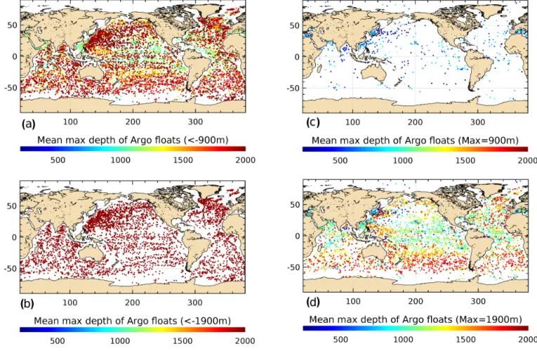
(Fig. 11c). The map of the discarded floats with a deep ref-erence level (1900 dbar) (Fig. 11d) indicates that floats with a mean max depth between 900 and 1400 dbar (in light blue and green) are mainly located at equatorial latitudes of all ocean basins. In these areas, the water column is very strati-fied and the steric signal is thus confined in the upper layer. Floats reaching depths between 1400 and 1900 dbar (in or-ange and light red) are mainly found at sub-polar latitudes where signals are more barotropic compared to lower lat-itudes (Luyten et al., 1983). Floats reaching depths deeper than 1900 dbar are relatively well spread out over the ocean with increasing density in the western boundary currents of the Northern Hemisphere. Thus, with a deep reference depth, the water column will be better sampled over the global ocean (which improves the retrieved steric signal) but we will miss a significant part of this steric signal, especially at equatorial latitudes. This illustrates the balance to be found between the horizontal (shallow reference level) and vertical (deep reference level) sampling of Argo floats.
3.7.2 Impact on the global MSL trend estimation An estimation of the global altimeter absolute drift is pro-vided by the global mean sea level differences between
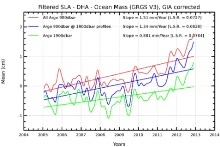
al-timetry and the sum of Argo steric heights with the GRACE ocean mass contribution. This is illustrated in Fig. 12 with various subsets of DHAs derived from the Argo network, al-lowing for the distinction of the effect of the horizontal and vertical sampling of the ocean by the floats. The altimeter drift estimated with all DHA from 900 dbar profiles (in red) is of 1.5 mm yr−1. Among these profiles, the selection of those whose maximum depth is at least 1900 dbar (impact of the horizontal sampling) has no impact in terms of global cor-relation between altimetry and Argo measurements (0.84 in both cases). There is a relatively low impact (−0.2 mm yr−1)
on the altimeter drift, which is reduced to 1.3 mm yr−1over
Figure 10.Taylor diagram of the steric contributions to the sea level derived from different sub-sampling of the Argo floats (DHAs ref-erenced to 900 dbar) with the mass contribution (GRACE GRGS) compared with the AVISO SSALTO/DUACS merged altimeter SLAs. For each sub-sampling of the in situ data set, the correspond-ing collocated altimeter measurements are used.
(horizontal sampling). As previously discussed with the anal-ysis of the sensitivity to the temporal and spatial sampling of the floats, this kind of sub-sampling associated with the reference level affects the estimation of the global absolute altimeter sea level trend. The 0.6 mm yr−1 total difference
observed between the shallow and deep reference levels in Fig. 12 is an estimation of one of the contributors to the error of the method of comparison.
3.7.3 Impact in terms of variance: altimetry multi- vs. mono-mission
We now describe two examples at global and regional scales illustrating that the comparisons of altimeter measurements with Argo in situ data in terms of variance are affected ac-cording to the reference level of integration of steric heights. At global scale, the Taylor diagram of Fig. 13 presents the correlation and the standard deviation of the differences be-tween altimeter multi-missions merged SLAs and the Argo steric DHAs. With a deep reference level (1900 dbar), the al-timeter (gray circle) and in situ (black circle) time series have the same standard deviation whereas a reduced variability is found with the in situ steric measurements referenced to a shallower level (900 dbar, black triangle). This reduced ver-tical sampling of the water column leads to a decrease of the
DHA standard deviation by a 0.85 factor at global scale. In addition, the correlation between both types of data is also deteriorated. This has to be taken into account when assess-ing the impact of a new altimeter standard or new product for instance.
At regional scales, Dhomps et al. (2011) reveal that the correlation and the regression coefficients between SLAs and DHAs vary spatially with a latitude dependency on the first order. In particular, their Fig. 5 suggests that the Southern Ocean is the place where the water column has to be sampled at the deepest level to estimate the steric signal. At high lati-tudes, the baroclinic signal below 1000 m depth significantly improves the correlation between SLAs and DHAs, the sea level variability being largely influenced by the deep baro-clinic signals. We illustrate this with Fig. 14 which indicates that the variances of the differences between altimeter SLAs and in situ DHAs are different whether the altimeter SLA is derived from mono-mission (TOPEX, Jason-1 and 2) or multi-missions grids of SLAs. In particular, with DHAs ref-erenced to 900 dbar (left panel), adding missions reduces the altimeter/Argo consistency in the high ocean variability ar-eas of the Antarctic Circumpolar Current (ACC) (blue, neg-ative values of−5 cm2on average). On the other hand, this tendency almost disappears in the ACC with the use of DHA referenced to 1900 dbar (right panel). This result is explained by the difference of variance of the water column as seen by altimetry or in situ data in this region. Figure 15 indicates that the variance of mono-mission and multi-missions altimeter products (collocated to Argo profiles) are very close to each other in the ACC but the variance of the Argo steric heights referenced at 900 dbar is significantly lower. Thus, with this reference level, both altimeter products cannot be distin-guished by comparison with Argo data. With a 1900 dbar reference level, the variance of the Argo steric heights be-comes similar to the values obtained with altimeter products in the ACC and the Argo measurements become relevant for the quality assessment of the altimeter products. This illus-trates that according to the ocean characteristics, the analysis of the variance of the water column and thus the differences between altimetry and Argo measurements are highly sensi-tive to the reference depth of integration of the Argo profiles.
3.8 Impact of the deep steric contribution
altime-Figure 11.Maps of the mean positions of Argo floats taken into account with a given reference depth(a, b)and the associated floats which will not be used because of their mean max depth shallower than the reference(c, d)for a 900 m(a, c)and a 1900 m(b, d)reference depth over the period 2005–2013.
ter SLAs with the sum of the steric signal and the ocean mass contribution, Dieng et al. (2015a) estimated the deep steric contribution (deeper than 1500 m) to be 0.3±0.6 and 0.55±0.6 mm yr−1 over the period 2005–2012 and 2003– 2012, respectively. Llovel et al. (2014) provided an estima-tion of 0.0±0.7 mm yr−1over the former period. The asso-ciated uncertainties include the formal error adjustment and the systematic errors associated with the observing system. The problem with the estimation of the deep steric contribu-tion is that it requires the knowledge of the steric contribucontribu-tion from the upper ocean and the comparison of different global steric sea level data sets indicates that a significant uncer-tainty remains on this estimation (Dieng et al., 2015a). This suggests that for the moment, there are still too large errors associated with the estimation of the deep steric contribution to detect absolute altimeter sea level drift with regards to cli-mate users requirements: 0.3 mm yr−1over 10-year (GCOS, 2011). Note that some deep profiling floats (about 4000 m) have been recently launched in the context of the Euro-Argo Improvements for Marine Services (E-AIMS D2.221, 2013) which should help to better characterize the deep steric con-tributions and assess their impact on the altimeter quality
Figure 12.Global mean sea level trends of the differences between the altimeter mean sea level (AVISO SSALTO/DUACS, 2014) and the steric plus mass (GRACE GRGS RL03 maps collocated with Argo profiles) contributions to the sea level with various subsets of DHAs derived from the Argo network: DHAs referenced to 900 dbar from all profiles reaching at least this pressure (red), DHA referenced to 900 dbar from the profiles reaching at least 1900 dbar (blue) and DHA referenced to 1900 dbar from all profiles reaching at least this pressure (green). All curves are 3-month low-pass fil-tered and a GIA correction is applied to altimeter (−0.3 mm yr−1) and ocean mass (−1.1 mm yr−1) measurements (Chambers et al., 2010; Tamisiea and Mitrovica, 2011).
Figure 13.Taylor diagram of the comparison of the sum of GRACE ocean mass and the steric Argo DHAs with a reference level at 900 dbar (triangle) and 1900 dbar (circle) with altimeter sea level time series (SSALTO/DUACS, 2014) (gray reference circle) on the xaxis over 2005–2013. The blue dotted lines indicate the normal-ized standard deviation (altimetry being the reference).
4 Conclusions
The internal consistency check and the comparison with other altimeter missions cannot systematically provide enough information for the quality assessment of altimeter sea level measurements. The in situ dynamic heights derived from the Argo network can be used as an independent refer-ence not only for the analysis of the relative mean sea level temporal evolution (including the detection of global and re-gional MSL drift and anomalies), but also for the detection of the impact of new altimeter standards or products used to calculate the sea surface heights. Our method constitutes an essential approach, which has a strong synergy with results derived from the altimetry comparison with tide gauges since the confrontation of both methods improves the confidence in the results. We have demonstrated that it is possible to detect altimeter drifts at global and regional scales and to charac-terize the impact of new altimeter standards. However, the improvements provided by these new standards and products become more and more reduced and the searched differences may be hidden by the errors of the method. It is thus neces-sary to better characterize the capacity of the method to dis-tinguish the performances of two altimeter products. Hence, this study focuses on the sensitivity of the altimeter/in situ sea level comparisons to different processing parameters.
The estimation of the absolute altimeter mean sea level drift requires the additional information related to the mass contribution to the sea level that can be derived from GRACE satellite measurements. Significant uncertainties are associ-ated with this data set, ranging from the GIA correction (0.3 mm yr−1), to the geocenter motion (0.1 mm yr−1), the fit
of the SH coefficients (0.1 mm yr−1) and the leakage from
land to the ocean (0.1 mm yr−1). The estimation of the
al-timeter MSL drift is thus directly affected by these uncer-tainties.
Sensitivity analyses performed on the Argo network have indicated that the spatial coverage of the ocean sampled by the instruments is significantly reduced as soon as a limited number of floats are used in the comparisons. However, this hardly affects the global correlation between altimeter SLAs and the in situ DHAs plus mass contribution, neither the vari-ance nor the trend of their differences. In addition, the 10-day temporal sampling of Argo floats was not designed for satel-lite altimetry validation purposes. We have shown that a re-duced temporal sampling of the floats can prevent us from detecting the impact of a new altimeter standard. The same diagnosis has been used to assess the impact of the reduction of the temporal and spatial sampling of Argo floats, leading to opposite conclusions. This suggests that the resulting dis-tributions of the in situ profiles (in space and time) are dif-ferent, leading to a different impact on the regional sea level trend estimation.
Figure 14.Map of the difference of variance of the altimeter SLA–Argo DHAs differences, using successively mono-mission and multi-missions grids of altimeter products with Argo 900 dbar profiles(a)and 1900 dbar profiles(b).
Figure 15.Temporal evolution of the standard deviation of the al-timeter SLA derived from mono-mission product (light blue), from multi-missions product (dark blue) and from Argo profiles with a 900 dbar reference (magenta) and 1900 dbar reference (red) in the Antarctic Circumpolar Current.
the ocean by Argo floats. A relatively deeper reference level can be assimilated to an additional sub-sampling effect since it allows for a better vertical sampling of the water column (more in agreement with what is seen by altimetry) but this leads to a reduced horizontal sampling of the ocean; the im-pact of the former being more than twice compared with the latter in terms of altimeter MSL trends estimation over a 8-years period. In some regions such as the Southern Ocean, the comparison with the altimeter sea level requires a deep reference depth so that the variance content of the water col-umn is similar between altimetry and in situ data.
Considering all the sources of errors discussed in this study including the method of collocation, the impact of the reference depth of Argo profiles, the uncertainty on GRACE ocean mass data sets and the error estimation on the deep steric contribution, this suggests that the uncertainty associ-ated with the obtained altimeter drifts is at least on the order
Figure 16.Time series of the DHAs derived from the profiles of float WMO 6901632 with different reference levels of integration varying from 900 dbar (red), 1900 dbar (blue), 3400 dbar (green) down to 4000 dbar (magenta) together with the collocated altime-ter SLAs (brown).
of 1.0 mm yr−1. The future evolution of the Argo network such as the deployment of deep Argo floats (4000 m) should contribute to improve the results and our approach will be an asset for the quality assessment of the recently launched Jason-3 and Sentinel-3 altimeters and the future SWOT mis-sion.
Data availability
The altimeter AVISO SSALTO/DUACS delayed-time sea surface height measurements from Pujol et al. (2016) are available at http://www.aviso.altimetry.fr/en/home.html. The climate-oriented monthly maps of altimeter sea level anoma-lies from the ESA climate change initiative (SL_cci v1.1; Cazenave and the Sea Level CCI team, 2014a) are ac-cessible under request at info-sealevel@esa-sealevel-cci.org and details are provided at http://www.esa-sealevel-cci.org. The temperature and salinity profiles from Argo floats were collected and made freely available by the International Argo Program (part of the Global Ocean Observing Sys-tem) and the national programs that contribute to it (http: //www.argo.ucsd.edu, http://argo.jcommops.org). Access to these data is available at http://www.coriolis.eu.org (Carval et al., 2015). The GRGS equivalent water heights of the GRACE ocean mass contribution to the sea level (Bian-cale et al., 2014) are available at http://grgs.obs-mip.fr/grace/ variable-models-grace-lageos/. The global mean ocean mass time series from GRACE RL05 (Johnson and Chambers, 2013) can be accessed at http://grace.jpl.nasa.gov.
Acknowledgements. This work was supported by the CNES thanks to the SALP project and was partly carried out as part of the FP7-SPACE E-AIMS project – grant agreement 312642. The authors thank D. Chambers and an anonymous reviewer for their comments which have contributed to improve the article and also Alejandro Blazquez for fruitful discussions.
Edited by: E. J. M. Delhez
References
Ablain, M., Cazenave, A., Valladeau, G., and Guinehut, S.: A new assessment of the error budget of global mean sea level rate esti-mated by satellite altimetry over 1993–2008, Ocean Sci., 5, 193– 201, doi:10.5194/os-5-193-2009, 2009.
Ablain, M., Cazenave, A., Larnicol, G., Balmaseda, M., Cipollini, P., Faugère, Y., Fernandes, M. J., Henry, O., Johannessen, J. A., Knudsen, P., Andersen, O., Legeais, J., Meyssignac, B., Picot, N., Roca, M., Rudenko, S., Scharffenberg, M. G., Stammer, D., Timms, G., and Benveniste, J.: Improved sea level record over the satellite altimetry era (1993–2010) from the Climate Change Initiative project, Ocean Sci., 11, 67–82, doi:10.5194/os-11-67-2015, 2015.
Arnault, S., Pujol, I., and Mélice, J. L.: In situ validation of Jason-1 and Jason-2 altimetry missions in the tropical Atlantic Ocean, Mar. Geod., 34, 319–339, 2011.
AVISO: Ssalto/Duacs user Handbook: (M)SLA and (M)ADT near-real time and delayed time products, SALP-MU-P-EA-21065-CLS ed. 4.1, 72 pp., 2014.
AVISO: Sea Surface Height from radar altimetry, AVISO SSALTO/DUACS, available at: http://www.aviso.altimetry.fr/ en/data/products/ocean-indicators-products/mean-sea-level/ processing-corrections.html, last access: 20 November 2015.
Biancale R., Lemoine, J.-M., Balmino, G., Bruinsma, S., Perosanz, F., Marty, J.-C., Loyer, S., Bourgogne, S., and Gégout, P.: 10 years of gravity variations from GRACE and LAGEOS data from CNES/GRGS, available at: http://grgs.obs-mip.fr/grace/ variable-models-grace-lageos (last access: 18 June 2015), 2014. Bonnefond, P., Exertier, P., Laurain, O., Menard, Y., Orsoni, A., Jan, G., and Jeansou, E.: Absolute calibration of Jason-1 and TOPEX/Poseidon altimeters in Corsica. Special Issue on Jason-1 calibration/validation, Mar. Geod., 26, 261–284, 2003.
Carval, T., Keeley, R., Takatsuki, Y., Yoshida, T., Schmid, C., Goldsmith, R., Wong, A., Thresher, A., Tran, A., Loch, S., and Mccreadie, R.: Argo user’s manual V3.2., doi:10.13155/29825, 2015.
Cazenave, A. and Sea Level CCI Team: ESA Sea Level Climate Change Initiative (ESA SL_cci): SEA LEVEL ESSENTIAL CLIMATE VARIABLE PRODUCTS, Version 1.1., December 2014, doi:10.5270/esa-sea_level_cci-1993_2013-v_1.1-201412, 2014a.
Cazenave, A., Dieng, H., Meyssignac, B., von Schuckmann, K., Decharme, B., and Berthier, E.: The rate of sea level rise, Nature Climate Change, 4, 358–361, doi:10.1038/NCLIMATE2159, 2014b.
Chambers, D. P., Wahr, J., and Nerem, R. S.: Preliminary obser-vations of global ocean mass variations with GRACE, Geophys. Res. Lett., 31, L13310, doi:10.1029/2004GL020461, 2004. Chambers, D. P., Tamisiea, M. E., Nerem, R. S., and Ries,
J. C.: Effects of ice melting on GRACE observations of ocean mass trends, Geophys. Res. Lett., 34, L05610, doi:10.1029/2006GL029171, 2007.
Chambers, D. P., Wahr, J., Tamisiea, M. E., and Nerem, R. S.: Ocean mass from GRACE and glacial isostatic adjustment, J. Geophys. Res., 115, B11415, doi:10.1029/2010JB007530, 2010.
Chambers, D. P., Cazenave, A., Champollion, N., Dieng, H., Llovel, W., Forsberg, R., Von Schukmann, K., and Wada, Y.: Evaluation of the Global Mean Sea Level Budget between 1993 and 2014, Surv. Geophys., special issue on integrative study of the mean sea level and its components, under review, 2016.
Chen J. L., Wilson, C. R., Chambers, D. P., Nerem, R. S., and Ta-pley, B. D.: Seasonal Global Water Mass Budget and Mean Sea Level Variations, Geophys. Res. Lett., 25, 3555–3558, 1998. Couhert, A., Cerri, L., Legeais, J. F., Ablain, M., Zelensky, P.,
Haines, N. P., Lemoine, B. J., Bertiger, F. G., Desai, D., and Ot-ten, M.: Towards the 1mm/y stability of the radial orbit error at regional scales, Adv. Space Res., doi:10.1016/j.asr.2014.06.041, online first, 2014.
CORIOLIS: Temperature and Salinity profiles from Argo floats, The CORIOLIS data service consortium, available at: http:// www.coriolis.eu.org, last access: 20 November 2015.
Dhomps, A. -L., Guinehut, S., Le Traon, P.-Y., and Larnicol, G.: A global comparison of Argo and satellite altimetry observations, Ocean Sci., 7, 175–183, doi:10.5194/os-7-175-2011, 2011. Dieng H. B., Palanisamy, H., Cazenave, A., Meyssignac, B., and
von Schuckmann, K.: The Sea Level Budget Since 2003: Infer-ence on the Deep Ocean Heat Content, Sur. Geophys., 36, 209– 229, doi:10.1007/s10712-015-9314-6, 2015a.
E-AIMS D2.221: deliverable report on deep float experiment de-sign, available at: http://www.euro-argo.eu/content/download/ 85564/1064777/file/E-AIMS_D2.221.pdf (last access: 24 June 2015), 2013.
England, M. H., McGregor, S.,Spence, P. , Meehl, G. A., Timmer-mann, A., Cai, W., Sen Gupta, A., McPhaden, M. J., Purich, A., and Santoso, A.: Recent intensification of wind-driven circula-tion in the pacific and the ongoing warming hiatus, Nature Cli-mate Change, 4, 222–227, 2014.
ESA: The Sea Level Climate Change Initiative (SL_cci) v1.1, Es-sential Climate Variable Cazenave et al. and Sea Level CCI team, available at: http://www.esa-sealevel-cci.org, last access: 20 November 2015.
Fasullo, J. T., Boening, C., Landerer, F. W., and Nerem, R. S.: Aus-tralia’s unique influence on global mean sea level in 2010–2011, Geophys. Res. Lett., 40, 4368–4373, doi:10.1002/grl.50834, 2013.
Fernandes, M. J., Lázaro, C., Ablain, M., and Pires, N.: Improved Wet Path Delays for all ESA and Reference altimetric missions, Remote Sens. Environ., 169, 50–74, 2015.
GCOS: Systematic Observation Requirements For Satellite-Based Data Products for Climate, available at: https://www.wmo. int/pages/prog/gcos/Publications/gcos-154.pdf (last access: 20 November 2015), 2011.
Geruo, A., Wahr, J., and Zhong, S.: Computations of the viscoelas-tic response of a 3-D compressible Earth to surface loading: an application to Glacial Isostatic Adjustment in Antarctica and Canada, Geophys. J. Int., 192, 557–572, doi:10.1093/gji/ggs030, 2013.
Guinehut, S., Le Traon, P.-Y., and Larnicol, G.: What can we learn from global altimetry/hydrography comparisons?, Geophys. Res. Lett., 33, L10604, doi:10.1029/2005GL025551, 2006.
Guinehut S., Coatanoan, C., Dhomps, A.-L., Le Traon, P.-Y., and Larnicol, G.: On the use of satellite altimeter data in Argo quality control, J. Atmos. Ocean. Tech., 26, 395–402, 2009.
Johnson, G. C. and Chambers, D. P.: Ocean bottom pressure sea-sonal cycles and decadal trends from GRACE Release-05: Ocean circulation implications, J. Geophys. Res.-Oceans, 118, 1–13, doi:10.1002/jgrc.20307, 2013.
Legeais, J.-F., Ablain, M., and Thao, S.: Evaluation of wet tropo-sphere path delays from atmospheric reanalyses and radiometers and their impact on the altimeter sea level, Ocean Sci., 10, 893– 905, doi:10.5194/os-10-893-2014, 2014.
Legeais J.-F., Guinehut, S., Prandi, P., Ablain, M., and Picot, N.: Analysis of altimetry errors using Argo and GRACE data, Poster presentation, 3658, European Geophysical Union, 2015a. Legeais J.-F., Guinehut, S., Prandi, P., Ablain, M., and
Desjon-quères, J.-D.: Analysis of altimetry errors using Argo and GRACE data, Poster presentation, OSTST meeting, availaible at: http://meetings.aviso.altimetry.fr/fileadmin/ user_upload/tx_ausyclsseminar/files/Poster_OSTST15_ AltimetryErrorsArgoGRACE_Legeais.pdf, last access: 20 November 2015b.
Llovel, W., Willis J. K., Landerer F. W., and Fukumori, I.: Deep-ocean contribution to sea level and energy budget not detectable over the past decade, Nature Climate Change, 4, 1031–1035, doi:10.1038/NCLIMATE2387, 2014.
Luyten, J. R., Pedlosky, J., and Stommel, H.: The Ventilated Ther-mocline, J. Phys. Oceanogr., 13, 292–309, doi:10.1175/1520-0485(1983)013<0292:TVT>2.0.CO;2, 1983.
Mitchum, G. T.: Monitoring the stability of satellite altimeters with tide gauges, J. Atmos. Ocean. Tech., 15, 721–730, 1998. Mitchum, G. T.: An improved calibration of satellite altimetric
heights using tide gauge sea levels with adjustment for land mo-tion, Mar. Geod., 23, 145–166, 2000.
Nerem, R. S., Chambers, D., Choe, C., and Mitchum, G.: Estimat-ing mean sea level change from the TOPEX and Jason altimeter missions, Mar. Geod., 33, 435–446, 2010.
Ollivier A., Faugere, Y., Picot, N., Ablain, M., Femenias, P., and Benveniste, J.: Envisat Ocean Altimeter Becoming Relevant for Mean Sea Level Trend Studies, Mar. Geod., 35, Supplement 1, 118–136, doi:10.1080/01490419.2012.721632, 2012.
Ponte, R. M., Quinn, K. J., Wunsch, C., and Heimbach, P.: A com-parison of model and GRACE estimates of the large-scale sea-sonal cycle in ocean bottom pressure, Geophys. Res. Lett., 34, L09603, doi:10.1029/2007GL029599, 2007.
Prandi P., Valladeau, G., Legeais, J. F., Ablain, M., and Picot, N.: Analysis of altimetry errors using in-situ measurements: Tide gauges and Argo profiles, Proceedings of the OSTST meeting, Boulder, available at: http://www.aviso.altimetry.fr/fileadmin/ documents/OSTST/2013/oral/prandi_InSitu_PP.pdf (last access: 20 November 2015), 2013.
Pujol, M.-I., Faugère, Y., Taburet, G., Dupuy, S., Pelloquin, C., Ablain, M., and Picot, N.: DUACS DT2014 : the new multi-mission altimeter dataset reprocessed over 20 years, Ocean Sci. Discuss., doi:10.5194/os-2015-110, in review, 2016.
Roemmich, D. and Gilson, J.: The 2004–2008 mean and annual cy-cle of temperature, salinity, and steric height in the global ocean from the Argo Program, Prog. Oceanogr., 82, 81–100, 2009. Roemmich, D. and Team, A. S.: Argo: The Challenge of Continuing
10 Years of Progress, Oceanography, 22, 46–55, 2009.
Rudenko, S., Dettmering, D., Esselborn, S., Schöne, T., Förste, C., Lemoine, J.-M., Ablain, M., Alexandre, D., and Neu-mayer, K.-H.: Influence of time variable geopotential mod-els on precise orbits of altimetry satellites, global and re-gional mean sea level trends, Adv. Space Res., 54, 92–118, doi:10.1016/j.asr.2014.03.010, 2014.
Schaeffer, P., Faugère, Y., Legeais, J. F., Ollivier, A., Guinle, T., and Picot, N.: The CNES-CLS11 Global Mean Sea Surface com-puted from 16 years of satellite altimeter data, Mar. Geod., 35, 3–19, 2012.
Stammer, D., Ray, R. D., Andersen, O. B., Arbic, B. K., Bosch, W., Carrièe, L., Cheng, Y., Chinn, D. S., Dushaw, B. D., Egbert, G. D., Erofeeva, S. Y., Fok, H. S., Green, J. A. M., Griffiths, S., King, M. A., Lapin, V., Lemoine, F. G., Luthcke, S. B., Lyard, F., Morison, J., Müller, M., Padman, L., Richman, J. G., Shriver, J. F., Shum, C. K., Taguchi, E., and Yi, Y.: Accuracy assessment of global barotropic ocean tide models, Rev. Geophys., 52, 243– 282, doi:10.1002/2014RG000450, 2014.
Swenson, S., Chambers, D., and Wahr, J.: Estimating geocenter variations from a combination of GRACE and ocean model out-put, J. Geophys. Res., 113, B08410, doi:10.1029/2007JB005338, 2008.
vari-ability, Oceanography, 24, 24–39, doi:10.5670/oceanog.2011.25, 2011.
Tapley, B. D., Bettadpur, S., Watkins, M., and Reigber, C.: The gravity recovery and climate experiment: Mission overview and early results, Geophys. Res. Lett., 31, L09607, doi:10.1029/2004GL019920, 2004.
Taylor, K. E.: Summarizing multiple aspects of model perfor-mance in a single diagram, J. Geophys. Res., 106, 7183–7192, doi:10.1029/2000JD900719, 2001.
Trenberth, K. E. and Fasullo, J. T.: An apparent hia-tus in global warming?, Earth’s Future, 1, 19–32, doi:10.1002/2013EF000165, 2013.
Valladeau G., Legeais, J. F., Ablain, M., Guinehut, S., and Pi-cot, N.: Comparing Altimetry with Tide Gauges and Argo Profiling Floats for Data Quality Assessment and Mean Sea Level Studies, Mar. Geod., 35, Supplement 1, 42–60, doi:10.1080/01490419.2012.718226, 2012.